HAL Id: hal-00296221
https://hal.archives-ouvertes.fr/hal-00296221
Submitted on 11 May 2007
HAL is a multi-disciplinary open access
archive for the deposit and dissemination of
sci-entific research documents, whether they are
pub-lished or not. The documents may come from
teaching and research institutions in France or
abroad, or from public or private research centers.
L’archive ouverte pluridisciplinaire HAL, est
destinée au dépôt et à la diffusion de documents
scientifiques de niveau recherche, publiés ou non,
émanant des établissements d’enseignement et de
recherche français ou étrangers, des laboratoires
publics ou privés.
lowermost stratosphere and their application to the
GMI chemistry and transport model
S. E. Strahan, B. N. Duncan, P. Hoor
To cite this version:
S. E. Strahan, B. N. Duncan, P. Hoor. Observationally derived transport diagnostics for the lowermost
stratosphere and their application to the GMI chemistry and transport model. Atmospheric Chemistry
and Physics, European Geosciences Union, 2007, 7 (9), pp.2435-2445. �hal-00296221�
www.atmos-chem-phys.net/7/2435/2007/ © Author(s) 2007. This work is licensed under a Creative Commons License.
Chemistry
and Physics
Observationally derived transport diagnostics for the lowermost
stratosphere and their application to the GMI chemistry and
transport model
S. E. Strahan1, B. N. Duncan1, and P. Hoor2
1Goddard Earth Science and Technology Center, University of Maryland, Baltimore County, Baltimore, MD 21250, USA 2Max Planck Institute for Chemistry, Air Chemistry, Mainz, Germany
Received: 8 January 2007 – Published in Atmos. Chem. Phys. Discuss.: 29 January 2007 Revised: 24 April 2007 – Accepted: 27 April 2007 – Published: 11 May 2007
Abstract. Transport from the surface to the lowermost stratosphere (LMS) can occur on timescales of a few months or less, making it possible for short-lived tropospheric pollu-tants to influence stratospheric composition and chemistry. Models used to study this influence must demonstrate the credibility of their chemistry and transport in the upper tropo-sphere and lower stratotropo-sphere (UT/LS). Data sets from satel-lite and aircraft instruments measuring CO, O3, N2O, and
CO2 in the UT/LS are used to create a suite of diagnostics
for the seasonally-varying transport into and within the low-ermost stratosphere, and of the coupling between the tropo-sphere and stratotropo-sphere in the extratropics. The diagnostics are used to evaluate a version of the Global Modeling Initia-tive (GMI) Chemistry and Transport Model (CTM) that uses a combined tropospheric and stratospheric chemical mech-anism and meteorological fields from the GEOS-4 general circulation model. The diagnostics derived from N2O and
O3show that the model lowermost stratosphere has
realis-tic input from the overlying high latitude stratosphere in all seasons. Diagnostics for the LMS show two distinct layers. The upper layer begins ∼30 K potential temperature above the tropopause and has a strong annual cycle in its compo-sition. The lower layer is a mixed region ∼30 K thick near the tropopause that shows no clear seasonal variation in the degree of tropospheric coupling. Diagnostics applied to the GMI CTM show credible seasonally-varying transport in the LMS and a tropopause layer that is realistically coupled to the UT in all seasons. The vertical resolution of the GMI CTM in the UT/LS, ∼1 km, is sufficient to realistically rep-resent the extratropical tropopause layer. This study demon-strates that the GMI CTM has the transport credibility re-quired to study the impact of tropospheric emissions on the stratosphere.
Correspondence to: S. E. Strahan
(sstrahan@pop600.gsfc.nasa.gov)
1 Introduction
Evaluation of transport between the upper troposphere (UT) and lower stratosphere (LS) is important because of the po-tential for tropospheric pollutants to impact stratospheric composition and chemistry. A decade ago, Ko et al. (1997) proposed that Bry produced from short-lived species in the
tropical UT may contribute to stratospheric halogen loading, and a recent study using BrO measurements and photochem-ical models supports this hypothesis (Salawitch et al., 2005). More recently, a “tape recorder” of CO forced by seasonal variations in biomass burning was identified in the tropical UT/LS using satellite CO measurements (Schoeberl et al., 2006). Tropospheric pollutants with lifetimes of only a few months can affect the composition of the lowest portions of the stratosphere.
There are two major transport pathways to the stratosphere (Holton et al., 1995; Dessler et al., 1995). In the tropics, con-vection brings boundary layer air up to ∼12 km (∼345 K), the base of the tropical tropopause layer (TTL) (Folkins, 2002). The TTL begins where convective mass flux falls off rapidly and extends to the cold point tropopause at 17–18 km (370–380 K) (Gettelman and Forster, 2002). Net heating rates become positive at about 16 km (∼360 K) in the TTL and ascent by the Brewer-Dobson circulation slowly lifts air up to and across the tropical tropopause and into the strato-sphere. A second pathway involves quasi-horizontal trans-port of air in the TTL to the extratropical lowermost strato-sphere (LMS). This pathway is aided by monsoon anticy-clones in the summer hemisphere (Chen, 1995), with pole-ward transport of tropospheric air on the west side and equa-torward transport of stratospheric air on the east side of the monsoonal circulation.
The lowermost stratosphere is defined as the region be-tween the extratropical tropopause, where isentropes con-nect the stratosphere and troposphere, and the stratospheric
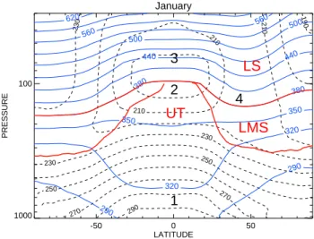
-50 0 50 LATITUDE 1000 100 PRESSURE January 190 210 210 210 230 230 230 250 250 270 270 290 290 290 320 320 350 350 380 380 440 440 500 500 560 560 620 1 2 3 4
LMS
UT
LS
Fig. 1. Schematic diagram of the UT/LS derived from zonal monthly mean GEOS-4 meteorological analyses from January 2005. Temperature contours are black (dashed) and potential tem-perature contours are blue. The lowermost stratosphere, bounded by the 380 K potential temperature surface and the 2 PVU surface, is outlined in red. Transport between the numbered regions is dis-cussed in the text.
overworld, where all isentropes are in the stratosphere (Fig. 1). This is the stratospheric part of the middleworld de-fined by Hoskins (1991). Air in the LMS has tropospheric and stratospheric origins, with the relative fractions vary-ing by season. In winter, large potential vorticity (PV) gra-dients near the subtropical jet form an elastic, nearly im-permeable barrier to cross-tropopause isentropic transport, much like that found at the edge of the polar vortex. Sub-tropical PV gradients are weaker in summer and evanes-cent waves from monsoonal circulations allow considerable stratosphere-troposphere exchange (STE) between the trop-ical UT and the LMS (Chen, 1995). Diagnostics of LMS transport, therefore, evaluate the integrated effects of the Brewer-Dobson (stratospheric) and monsoon (tropospheric) circulations.
There is agreement in the chemistry-climate model com-munity on the need for diagnostics in the middleworld (Eyring et al., 2005). Numerous trace gas measurements in this region have large or seasonally-varying gradients across the tropopause, making them excellent indicators of the strength and timing of the dynamical processes affecting the middleworld. For example, Ray et al. (1999) used CO2
and CFC-11 profiles to demonstrate that the LMS compo-sition changes from primarily stratospheric to tropospheric air between spring and fall. Similarly, Hoor et al. (2002) noted differences in the CO-O3 correlation between
win-ter and summer that indicated increased influence of tropo-spheric air in the LMS in July. Recently, Pan et al. (2007) have developed diagnostics for transport processes near the extratropical tropopause based on CO, O3, H2O, and
varia-tions in their mixing lines.
In this paper, we present diagnostics of middleworld trans-port and composition derived from satellite and aircraft mea-surements of CO, CO2, N2O, and O3. Relevant dynamical
processes include the ascent of tropical air from the surface to the stratosphere, the seasonally-varying transport from the tropical UT to the LMS, and the coupling between the ex-tratropical UT and LMS. We also present a new version of the Global Modeling Initiative (GMI) chemistry and trans-port model (CTM) that uses meteorological fields from the GEOS-4 general circulation model (GCM) (Bloom et al., 2005) and has a chemical mechanism that includes tropo-spheric and stratotropo-spheric chemical reactions. The diagnos-tics are applied to this CTM, establishing the credibility of its UT/LS transport and supporting its use in studies of the im-pact of tropospheric emissions on lower stratospheric com-position.
2 Model and simulation descriptions
The GMI CTM used in this study is related to the version de-scribed in Douglass et al. (2004) and references therein. The CTM uses a flux form semi-Lagrangian numerical transport scheme (Lin and Rood, 1996). The version of the model used here, referred to as the “GMI Combo”, has a chemical mech-anism that combines the stratospheric mechmech-anism described in Douglass et al. (2004) with a modified version of the tropo-spheric mechanism originating in the Harvard GEOS-CHEM model (Bey et al., 2001). This combined mechanism con-tains 113 chemically active species, 315 chemical reactions and 78 photolytic processes. A new version of the Fast-J2 photochemical solver (Bian and Prather, 2002) called Fast-JX includes more bins for the calculation of stratospheric photolysis rates. Photolysis frequencies are computed using the Fast-JX radiative transfer algorithm, which combines the Fast-J tropospheric photolysis scheme described in Wild et al. (2000) with the Fast-J2 stratospheric photolysis scheme of Bian and Prather (2002) (M. Prather, personal commu-nication, 2005). The scheme treats both Rayleigh scatter-ing as well as Mie scatterscatter-ing by clouds and aerosols. The SMVGEAR II solver uses a 30-min timestep for the chem-istry calculation, which is more accurate near the termina-tor than the 1-h timestep used in previous studies. Perfor-mance metrics of SMVGEAR II with respect to other solvers in the GMI stratospheric CTM can be found in Rotman et al. (2001). Model representation of physical processes in the troposphere, such as convection, wet scavenging, and dry de-position, are described in Duncan et al. (2007).
Long-lived source gases, such as N2O, CH4, and the
halo-carbons, are forced at the two lowest levels with a mixing ratio boundary condition updated monthly, based on the A2 scenario (WMO, 2003). A climatology is used to specify the stratospheric distribution of water vapor each month. The GMI CTM calculates a change in water from the specified trend in methane and adds this to the climatology of each
time step. CO2 is forced at the two lowest levels with a
mixing ratio boundary condition using a time series derived from global surface observations (Conway et al., 1994) from a 17-yr period. The CO2boundary condition has 10◦-wide
latitude bins with no longitudinal variability and is updated monthly. Model CO sources include emissions from biomass burning, fossil fuel consumption, biofuel use, lightning, and biogenics. They are treated as fluxes rather than mole frac-tion boundary condifrac-tions and are described in Duncan et al. (2007). This mechanism lacks a high altitude loss for CO2, a source of CO, and thus the model CO is biased low
in the stratosphere.
The CTM simulation evaluated here was run with meteo-rological fields from a 5-yr integration of the GEOS-4.0.2 GCM (Bloom et al., 2005). This integration was forced by observed sea surface temperatures for the period 1994– 1998. The native resolution of the meteorological fields is 2◦ latitude by 2.5◦ longitude and 55 vertical levels with a
lid at 0.015 hPa. The resolution in the UT/LS is ∼1 km. To shorten the CTM integration time, the 24 levels above 10 hPa were mapped to 11 levels using the method of Lin (2004); the top level is unchanged. The resulting CTM grid is 2◦latitude×2.5◦longitude by 42 levels. A study of the
ef-fects of resolution and lid height on CTM transport character-istics determined that transport in the lower stratosphere and below is negligibly impacted by reduced resolution above 10 hPa (Strahan and Polansky, 2006).
3 Transport diagnostics in the upper troposphere and lower stratosphere
Evaluation of the stratosphere in a CTM simulation inte-grated with meteorological fields from a GCM essentially evaluates extratropical wave driving in the GCM, the driver of the stratospheric circulation. A GCM that correctly simu-lates the generation, propagation, and dissipation of Rossby waves may correctly represent the global scale aspects of transport and STE (Holton et al., 1995). However, composi-tion of the LMS depends on the interaccomposi-tion of UT processes with the Brewer-Dobson circulation. Thus, the diagnostics presented here evaluate the integrated effect of stratospheric and tropospheric processes on the UT/LS.
3.1 Transport up to and through the tropical tropopause Changes in the amplitude and phase of the CO2 cycle
ob-served at points 1 through 4 in Fig. 1 provide the basis for a series of transport diagnostics. Boering et al. (1996) (here-inafter referred to as B96) used ground-based CO2
measure-ments (Conway et al., 1994) along with NASA ER-2 aircraft data to estimate transport rates from the surface to the trop-ical tropopause, and from the troptrop-ical LS to the midlatitude LS. Figure 2 uses the B96 analysis to evaluate model trans-port from the surface to the tropical UT and beyond. B96
Surface to Tropical Tropopause
Jan Apr Jul Oct Jan Apr Jul Oct Jan 350 352 354 356 358 Detrended CO 2 (ppm)
Mauna Loa + Samoa (Surface Avg)
Strat Entry
2-Month Lag
A
Tropical Tropopause to 435K
Jan Apr Jul Oct Jan Apr Jul Oct Jan 351 352 353 354 355 356 357 Detrended CO 2 (ppm) Strat Entry (380K) 435 K 2.5-Month Lag
B
Tropics to Midlatitudes - 390KJan Apr Jul Oct Jan Apr Jul Oct Jan 353 354 355 356 357 358 359 CO 2 (ppm) Tropics 36-40N
C
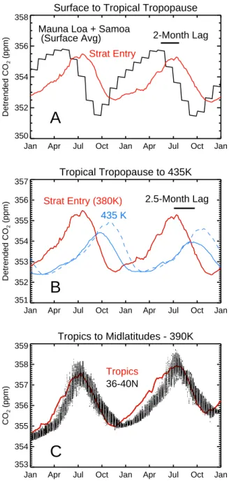
Fig. 2. Zonal mean CO2seasonal cycles from two years of the GMI Combo CTM with the annual trend removed. (a) The black line is the average of Mauna Loa and Samoa model boundary conditions (derived from the NOAA Global Monitoring Division Flask Sam-pling Network) and the red line is the model tropical CO2at the point of stratospheric entry (380 K). (b) The model tropical CO2at stratospheric entry (380 K, red) is compared with the tropical cycle at 435 K (solid blue); there is a 2.5 month lag between them. The dashed blue line approximates how the model cycle should look if the attenuation and lag followed the aircraft results from B96. (c) The model tropical CO2 near stratospheric entry (red) and in the midlatitudes (black lines show variability), 380–400 K. In this panel, the annual trend is not removed because it does not hinder comparison of the amplitudes.
showed that the seasonal cycle at tropical stratospheric en-try (380–390 K) could be represented by the average of the surface cycles measured at Mauna Loa (19◦N) and Samoa
(14◦S) time lagged by 2 months (Fig. 2a); this is the
trans-port between points 1 and 2 in Fig. 1. The model results shown in Figs. 2a–b have the annual trend removed in order to clearly show the amplitude. The solid black line is the av-erage of the model surface forcing at Mauna Loa and Samoa, which was derived from global observations (Conway et al., 1994). The model cycle at the tropical tropopause (red) is realistically lagged by 2 months, however, the amplitude is ∼1 ppm less than observed by B96. This appears to be due the surface minimum (fall) arriving with a ∼1 ppm increase in CO2. From the tropical tropopause, B96 found that the
cycle was transported upward to ∼435 K in 3–4 months, di-minished in amplitude by 20%.; this is the transport between points 2 and 3 in Fig. 1. If the model cycle at the tropopause (Fig. 2b, red) showed the same behavior, it would produce a cycle at 435 K shown by the dashed blue line in Fig. 2b. The actual model cycle at 435 K is shown by the solid blue line, which indicates that ascent is too rapid (the lag is 2.5 months) and that attenuation or horizontal exchange in the LS is too great, with ∼40% loss of amplitude instead of 20%. The loss of amplitude occurs during the ascent of the cycle maximum in late summer and fall, suggesting that the Brewer-Dobson circulation may be too strong in these seasons. Schoeberl et al. (2006) also assessed tropical ascent and horizontal mix-ing in this model from 14–20 km by comparison with the observed CO “tape recorder”. They found that the model agreed well with the observed tilt of the CO signal (ascent rate) and the height at which the signal faded (horizontal mix-ing convolved with CO lifetime). While the tape recorder evaluation was only qualitative, it suggested that ascent and mixing throughout the year were roughly correct. The CO2
phase and attenuation comparison shown here is a stricter test of these processes and shows good agreement from mid-winter to early summer, but suggests excess strength in late summer and fall.
B96 also examined poleward horizontal transport in the LS; this is the transport between points 2 and 4 in Fig. 1. Their CO2 analysis used potential temperature and
co-located N2O mixing ratios to create a vertical coordinate that
effectively followed the extratropical tropopause, similar to the approach taken by Hoor et al. (2004), hereinafter referred to as H2004. They found that the CO2 cycle observed at
the tropical tropopause could also be found near ∼38◦N,
undiminished, with no more than a 1-month time lag. Fig-ure 2c shows the model CO2cycles in the tropics and from
36–40◦N, sorted by N
2O=305–310 ppb and potential
tem-perature (theta)=380–400 K, just as in the B96 analysis. The near perfect match of the phase and amplitude of these cycles suggests realistic poleward transport in the lowest part of the stratospheric overworld. Notice that there is no lag in sum-mer and fall, but roughly a 1 month lag in winter and spring. This is consistent with transport variations in the LMS
de-scribed by Chen (1995) and Dunkerton (1995), who showed stronger exchange between the tropics and midlatitudes oc-curring in summer.
3.2 The seasonally-varying composition of the lowermost stratosphere
Several analyses have shown that the composition of the LMS varies considerably between winter and summer (e.g., Ray et al., 1999; Hoor et al., 2002; H2004; Krebsbach et al., 2006 and Hegglin et al., 2006). In winter and spring, the LMS has stratospheric character due to strong down-ward motion at mid and high latitudes, while large PV gra-dients across the subtropical jet restrict cross-tropopause transport. In summer, when downward advection by the Brewer-Dobson circulation is weak, the LMS has greater tro-pospheric character due to weak subtropical PV gradients which allow enhanced horizontal transport from the tropical UT to the LMS by the monsoonal anticyclones (Chen, 1995). Ozone and N2O are useful as tracers of the origin of air
because of their gradients across the tropopause. N2O and
O3have opposite source regions, the troposphere and
strato-sphere, respectively, and are long-lived in the LMS. Several datasets will be used to examine seasonal variations in lower stratospheric composition. The Microwave Limb Sounder (MLS) on the NASA Aura satellite provides daily measure-ments from 82◦S–82◦N for O
3 (215 hPa and above) and
N2O (100 hPa and above) (Waters et al., 2006). MLS
verti-cal resolution is ∼3 km in the LS and ∼4 km on the 215 hPa surface (middleworld). MLS N2O at 100–68 hPa shows
oc-casional high bias estimated to be generally less than 10%; MLS O3has a reported bias of 1% in the stratosphere and ∼10% in the UT, and biases of 30–40% at pressures 200-300 hPa (Livesey et al., 2005). N2O data from eight SPURT
aircraft campaigns are available in the extratropical LMS in all seasons (Engel et al., 2006). Seasonal mean analyses of ER-2 N2O and O3data (Strahan et al., 1999; Strahan, 1999)
provide profiles and latitudinal gradients from 360–500 K. All aircraft data are used in equivalent latitude/potential tem-perature coordinates to eliminate spatial biases that may be caused by limited longitudinal sampling. Use of equivalent latitude extends the effective latitude range sampled by both aircraft to ∼87◦N. We use a dynamical definition of the
tropopause, 2 PVU, where 1 PVU=10−6m2K s−1kg−1, to
define the lower boundary of the LMS. 3.2.1 N2O
The composition of the polar LS directly affects the LMS through downward transport by the Brewer-Dobson circula-tion. Low N2O descends in winter and spring, while in
sum-mer LMS composition is influenced by horizontal transport of higher (tropospheric) N2O from low latitudes. Figure 3
shows area-weighted contoured pdfs of model N2O and the
Winter 0 50 100 150 200 250 300 350 N2O (ppb) 300 350 400 450 500 Potential Temperature (K) Spring 50 100 150 200 250 300 350 N2O (ppb) 300 350 400 450 500 Potential Temperature (K) Summer 100 150 200 250 300 350 N2O (ppb) 300 350 400 450 500 Potential Temperature (K) Fall 100 150 200 250 300 350 N2O (ppb) 300 350 400 450 500 Potential Temperature (K) 0.000 0.001 0.010 0.020 0.060 0.100 0.200 0.300 Probability
Fig. 3. Comparison of GMI and MLS high latitude N2O profiles (70–82◦N) in four seasons with SPURT and ER-2 profiles. GMI area-weighted contoured pdfs are calculated over the same seasonal sampling periods of the SPURT data (all months of the year except March, June, September, and December). Yellows and reds indicate sharply peaked distributions. MLS data are shown as most proba-ble seasonal profiles (black line). ER-2 data (black diamonds) and SPURT data (blue diamonds) are seasonal means for equivalent lat-itudes 70◦N–88◦N.
for latitudes 70◦–82◦N. Also plotted are seasonal mean N
2O
profiles from ER-2 (black diamonds) and SPURT (blue di-amonds) analyses with equivalent latitudes 70◦–88◦N. The
most probable values in winter represent the model mean vortex profile, while the large variability comes from pro-files outside the vortex. (The spring ER-2 data are omitted because they are from 1997, a year with an unusually late vortex breakup (Coy et al., 1997).) The only disagreement with the data is found in summer and fall above 450 K, where the model is up to 15% too high. Although the strength of de-scent and horizontal mixing cannot be judged independently, the excellent model agreement throughout most of the year at levels as low as 320 K suggests a very good balance of ver-tical and horizontal transport at levels of the polar LS affect-ing the LMS. The SPURT measurements are higher than the model in the LMS in winter, but this could be due to weaker descent in the warm Arctic winters during the SPURT cam-paigns (2002 and 2003). The model Arctic temperatures are near or below the real climatological mean.
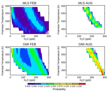
Variability is an indicator of recent transport processes. In winter, large tracer gradients across the vortex edge coupled with wave-driven vortex displacements create high latitude pdfs showing large variability. Strong horizontal mixing in spring causes breakdown of the vortex and homogenization of long-lived trace gases in the extratropics. In summer, the well-mixed extratropics produce pdfs with very low variabil-ity because wave-driving is weak. Figure 4 shows contoured
MLS FEB 0 100 200 300 N2O (ppb) 450 500 550 600 Potential Temperature (K) GMI FEB 0 100 200 300 N2O (ppb) 450 500 550 600 Potential Temperature (K) MLS AUG 0 100 200 300 N2O (ppb) 450 500 550 600 Potential Temperature (K) GMI AUG 0 100 200 300 N2O (ppb) 450 500 550 600 Potential Temperature (K) 0.000 0.005 0.010 0.025 0.050 0.075 0.100 0.150 0.200 Probability
Fig. 4. Comparison of GMI and MLS winter and summer high latitude N2O profile variability (66◦–82◦N). MLS data are from 2005 and 2006. GMI variability is shown from two consecutive model years.
pdfs of MLS and GMI N2O profiles between 66◦–82◦N in
winter and summer, demonstrating the realistic seasonal vari-ability of high latitude transport and mixing processes in the GMI Combo CTM. In February, excellent agreement be-tween MLS and the model most probable profiles inside and outside the vortex, as well as the variability in both regions, shows that the model vortex is well isolated. The model has more mixing ratios between the two profiles, indicating slightly more mixing across the vortex edge. In summer, the MLS data and the model both show low variability charac-teristic of a well-mixed atmosphere with little wave-driving. Close agreement with MLS variability is also seen in the months not shown. Together, the comparisons in Figs. 3 and 4 are an important demonstration that LS transport processes in the GMI Combo CTM LS are credible and provide realis-tic input for the LMS in all seasons.
To examine seasonally-varying transport and composition in the LMS, we look at SPURT N2O in the dynamical
co-ordinate system of equivalent latitude and potential temper-ature. We use equivalent latitude, which maps each mea-surement onto latitude according to its potential vorticity, because it removes variability caused by reversible wave transport (Butchart and Remsberg, 1986; Nash et al., 1996). H2004 and Hegglin et al. (2006) used this coordinate sys-tem to show that the isopleths of CO, N2O, and O3 follow
PV rather than potential temperature contours in the LMS (<360 K) in all seasons.
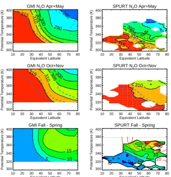
GMI and SPURT N2O in the spring and fall, shown in
Fig. 5, illustrate the seasonally changing composition of the LMS; the dashed lines overlays are PV contours (2, 4, and 6 PVU). Note that the PV contours cross isentropes, that is,
GMI N2O Apr+May 10 20 30 40 50 60 70 80 Equivalent Latitude 300 320 340 360 380 400 Potential Temperature (K) 280 290 300 305 310 315 SPURT N2O Apr+May 10 20 30 40 50 60 70 80 Equivalent Latitude 300 320 340 360 380 400 Potential Temperature (K) 300 305 310 315 GMI N2O Oct+Nov 10 20 30 40 50 60 70 80 Equivalent Latitude 300 320 340 360 380 400 Potential Temperature (K) 300 305 310 315 SPURT N2O Oct+Nov 10 20 30 40 50 60 70 80 Equivalent Latitude 300 320 340 360 380 400 Potential Temperature (K) 310
GMI Fall - Spring
10 20 30 40 50 60 70 80 Equivalent Latitude 300 320 340 360 380 400 Potential Temperature (K) 5 10 15
SPURT Fall - Spring
10 20 30 40 50 60 70 80 Equivalent Latitude 300 320 340 360 380 400 Potential Temperature (K) 0 5 10 10 10 15 20 25 30 5 10 15
Fig. 5. Comparison of GMI and SPURT N2O in spring (April and May) and fall (October and November) in the lowermost strato-sphere. Potential vorticity contours (2, 4, and 6 PVU) are overlaid with dashed blue lines. The bottom panels show the fall-spring dif-ference. The bottom right panel (SPURT) shows the model differ-ences overlaid in red.
there are PV gradients on the isentropic surfaces. The PV gradients hinder isentropic transport, allowing time for di-abatic cooling in the middleworld to move tracer isopleths downward as they are transported poleward. This is equiva-lent to the barrier to isentropic transport reported in Hegglin et al. (2006). The model N2O isopleths, like the data,
fol-low the PV contours near the tropopause much more closely rather than they do isentropic surfaces, suggesting that the model has a reasonable balance between horizontal transport and diabatic cooling here. In all seasons except winter, model N2O mixing ratios are always within 2% of SPURT values.
As noted before, SPURT values may be relatively high in winter due to weak descent in the observation years.
Composition differences between spring and fall are shown in the bottom panels of Fig. 5. In spring, downward advection by the Brewer-Dobson circulation is at a maxi-mum, resulting in relatively low N2O, and in fall, the
down-ward circulation is weak while the influence of horizontal transport of high N2O from the TTL is greatest. This is
con-sistent with the upper middleworld (≥350 K) results of Chen (1995), where seasonal mixing across the subtropical jet was found to be enhanced by the summer monsoon circulations. The composition difference is proportional to the seasonally changing tropospheric fraction of air in the LMS and is well represented by the model as a function of both height and latitude up to ∼360 K, where the model appears to be less tropospherically influenced than the SPURT data.
3.2.2 Ozone
Ozone is also an excellent lower stratospheric transport tracer and use of its seasonal cycles has been advocated for the eval-uation of model transport in the LMS (Logan, 1999). The availability of daily global MLS O3measurements down to
215 hPa allows evaluation of the entire middleworld. Ozone in this region is controlled largely by transport, although O3
production and loss are sensitive to local NOx.
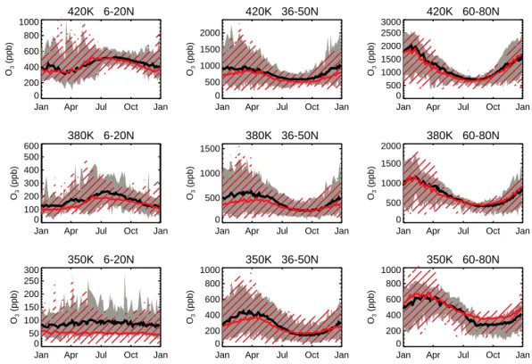
Figure 6 shows the annual cycle of O3 from the tropics
to high latitudes, from 350–420 K using MLS data (black); GMI O3 is overlaid in red. The solid lines represent the
mean values over the given latitude ranges, while the shad-ing or hatchshad-ing shows the full range of the variability. ER-2 data are not used here because they are only available as seasonal means. GMI O3 shows close agreement with the
observed MLS annual cycles and their variability, within the range of uncertainty reported for these data (Livesey et al., 2005). GMI O3 in the tropical UT is 30–50 ppb lower than
the MLS data, but as the MLS data may be biased between 10–40% at 215 hPa, a level that contributes to the 350 K sur-face, there is no definitive disagreement here. Simulated O3
agrees much more closely with the ozonesonde climatology of Logan (1999), where tropical O3was found to range from
30–90 ppb at 200 hPa, and with the tropical ozonesonde cli-matology of Folkins et al. (2006), where an average of 40– 80 ppb was found in the TTL. Agreement at 380 K in the tropics is within the 10% uncertainty reported for the MLS UT measurements. GMI high latitude O3shows near perfect
agreement in all seasons at all levels shown, except for the 350 K surface in summer and fall, where again, the 30–40% MLS bias in 215 hPa data could be a factor. GMI midlatitude O3looks good in summer and fall but is low in winter. If the
vortex were too isolated, the amount of high O3mixed into
the midlatitudes would be too low; however, Fig. 4 shows that the vortex is not overly isolated. If GMI tropical O3is
truly low, this could indicate too much transport to midlati-tudes. Insufficient midlatitude descent, which has not been evaluated here, is also a possible cause. Overall, the agree-ment between observed and GMI mean O3and its
variabil-ity in the middleworld and LS is quite close, particularly in the context of the large range of mixing ratios observed here (∼100–2500 ppb). Because variability and seasonal compo-sition are controlled primarily by transport, the O3and N2O
diagnostics demonstrate credible model transport throughout the year in the extratropical lower stratosphere from 320– 500 K.
3.3 Stratosphere-troposphere coupling at the extratropical tropopause
3.3.1 CO
CO has tropospheric sources and a lifetime of several months in the UT and LMS (Duncan et al., 2007). H2004 found
420K 6-20N
Jan Apr Jul Oct Jan
0 200 400 600 800 1000 O3 (ppb) 420K 36-50N
Jan Apr Jul Oct Jan
0 500 1000 1500 2000 O3 (ppb) 420K 60-80N
Jan Apr Jul Oct Jan
0 500 1000 1500 2000 2500 3000 O3 (ppb) 380K 6-20N
Jan Apr Jul Oct Jan
0 100 200 300 400 500 600 O3 (ppb) 380K 36-50N
Jan Apr Jul Oct Jan
0 500 1000 1500 O3 (ppb) 380K 60-80N
Jan Apr Jul Oct Jan
0 500 1000 1500 2000 O3 (ppb) 350K 6-20N
Jan Apr Jul Oct Jan
0 50 100 150 200 250 300 O3 (ppb) 350K 36-50N
Jan Apr Jul Oct Jan
0 200 400 600 800 1000 O3 (ppb) 350K 60-80N
Jan Apr Jul Oct Jan
0 200 400 600 800 1000 O3 (ppb)
Fig. 6. Comparison of GMI (red) and MLS (black) O3seasonal cycles for three latitude bands and 3 levels in the UT/LS. Solid lines are averages of all longitudes within the latitude band while the shading shows the full range of variability.
that SPURT CO profile data analyzed as a function of height relative to the dynamical tropopause (“delta theta”) showed three distinct regions. At potential temperatures 25 K or more above the extratropical dynamical tropopause, defined as 2 PVU, they observed low CO mixing ratios and low variabil-ity characteristic of stratospheric air. Below the tropopause they observed high CO mixing ratios typical of the tropo-sphere. From just below the tropopause to 25 K above it, a mixed layer was found that connected the two regions. The mixed layer had nearly constant thickness in all seasons and at all extratropical latitudes, although in summer it may have been slightly thicker (∼30 K). On an absolute scale, the mixed layer was almost always below the 350 K surface during the SPURT campaigns at latitudes 50◦N or higher.
These results are consistent with the tracer studies of Chen (1995), who reported that vigorous exchange between the stratosphere and troposphere occurred year-round at 330 K and below due to breaking synoptic scale baroclinic distur-bances. H2004 concluded that the thickness of the mixed layer near the tropopause was a measure of the coupling be-tween the stratosphere and troposphere. A recent analysis of CO and O3high latitude aircraft measurements by Pan et
al. (2007) determined that a well-defined mixed layer ∼2 km thick extended across the thermal tropopause. A 2-km layer near the tropopause spans ∼25 K potential temperature, mak-ing this result consistent with the H2004 findmak-ings.
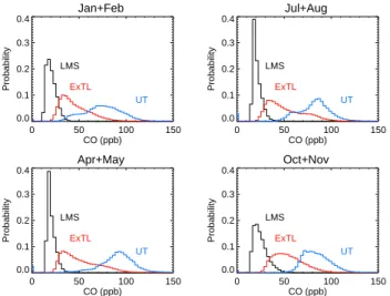
We apply the results of the H2004 CO profile analy-sis to diagnose model extratropical stratosphere-troposphere coupling. To identify tropospheric or stratospheric charac-ter in the model, we evaluate histograms calculated from model CO in the 3 regions identified by the SPURT CO analysis: below the tropopause (≤−10 K), the tropopause mixed layer (−10 K to 25 K), and the LMS (≥25 K above the tropopause). Figure 7 shows histograms for the sea-sons sampled by SPURT. The model distributions in the UT have mean values of 80–90 ppb and show large variability. The distributions ≥25 K above the tropopause (LMS) are sharply peaked at ∼20 ppb, characteristic of stratospheric (aged) air. Notice that the UT and LMS distributions are al-most completely non-overlapping indicating the distinctive-ness of these regions. The extratropical tropopause layer (ExTL) has a CO peak of 30–40 ppb, which is closer to the stratospheric mean, but has a long tail with higher (tropo-spheric) CO mixing ratios. The ExTL distribution clearly has features that indicate a mixture of stratospheric and tro-pospheric air. The slight overlap of LMS and UT distribu-tions in winter suggests that the model mixed layer extends a little higher than 25 K above the tropopause in this season.
We find that the thickness of the model mixed layer, like the results of the SPURT analysis (H2004), extends to ∼25 K above the dynamical tropopause in all seasons. This diag-nostic suggests that the GEOS4-GCM meteorological fields used in the GMI Combo CTM provide reasonable forcing by
Jan+Feb 0 50 100 150 CO (ppb) 0.0 0.1 0.2 0.3 0.4 Probability LMS ExTL UT Apr+May 0 50 100 150 CO (ppb) 0.0 0.1 0.2 0.3 0.4 Probability LMS ExTL UT Jul+Aug 0 50 100 150 CO (ppb) 0.0 0.1 0.2 0.3 0.4 Probability LMS ExTL UT Oct+Nov 0 50 100 150 CO (ppb) 0.0 0.1 0.2 0.3 0.4 Probability LMS ExTL UT
Fig. 7. Histograms of GMI Combo CO in the extratropical UT/LMS in four seasons. The UT distributions show points 10–50 K below the 2 PVU tropopause. The ExTL contains points from 10 K below to 25 K above the tropopause and the LMS distributions contain points from 25–80 K above the tropopause.
synoptic scale disturbances in the UT throughout the year to couple the troposphere with the lowest layers of the strato-sphere. This also shows that the resolution of the GMI Combo CTM, 2◦latitude×2.5◦longitude in the horizontal
and ∼1 km (∼12 K) in the vertical in the UT/LS, is sufficient to represent realistic coupling at the extratropical tropopause. 3.3.2 CO2
The CO2seasonal cycle phase and amplitude at the
extratrop-ical tropopause not only demonstrate the coupling between troposphere and stratosphere, but can be used to diagnose the influence of air arriving via the tropical stratosphere at levels above the coupling. Observed CO2cycles in the UT
and at the tropopause have a spring maximum and a large amplitude, but in the LMS the amplitude is much lower and the maximum occurs several months later (Nakazawa et al., 1991; B96; H2004). As has been demonstrated by analysis of observations in B96, Strahan et al. (1998), and H2004, the LMS cycle arrives via ascent through the tropical tropopause, followed by meridional poleward transport. The seasonal maximum that occurs in May in the northern mid-high lat-itude lower troposphere requires ∼3 months to travel to the midlatitude LS via the tropical tropopause. H2004 observed that this transport pathway results in a reversed CO2
verti-cal gradient across the tropopause in late summer. The ob-servations used in all of these analyses were collected over many decades, while CO2increased at variable growth rates.
Because aircraft measurements are sporadic in time and lo-cation, the phases and amplitudes of the cycles were deter-mined from two or more years of observations in the anal-yses referenced. For these reasons, it makes more sense to
GMI CO2 45-60N
Jan Apr Jul Oct Jan
352 354 356 358 360 CO 2 (ppm) UT (-30K - -10K) Tropopause (-10K - 10K) 10K - 30K 30K - 50K 50K - 70K
Fig. 8. GMI CO2 cycles below, at, and above the midlatitude tropopause (2 PVU), 45–60◦N. Each seasonal cycle is calculated over a 20 K-wide vertical coordinate defined by the distance in po-tential temperature from the tropopause. The black dashed line marks the month when SPURT data show a reversed vertical gra-dient (H2004).
use the results of these analyses, rather than the observations themselves, for evaluating models.
Figure 8 shows the model CO2 cycles at several levels
above and below the 2 PVU tropopause using the same ‘delta theta’ coordinate as H2004. The model cycles are computed by finding each grid point’s distance in potential temperature from the 2 PVU level, binning those points into 20 K wide bins centered from −20 K to +60 K above the tropopause, then averaging over 45◦–60◦N and all longitudes. In the
UT and at the tropopause (blue), the model’s cycles share two essential features of the analyzed UT observations: a large amplitude cycle (∼6 ppm) and a spring maximum. Just above the tropopause (green), the amplitude is much lower and the maximum occurs more than 1 month later. These fea-tures suggest a mixture of influences from above and below, consistent with the mixed layer diagnosed by the CO distri-butions (Fig. 7). At 30–70 K above the tropopause (orange and red), the cycle amplitudes are slightly greater than in the mixed layer (10–30 K) and the maximum is shifted to late summer. The higher amplitude is a characteristic of trans-port via the tropical tropopause and is seen at 40–60 K above the tropopause by H2004. The phase delay is also charac-teristic of this transport pathway and was observed in all the previously referenced CO2studies. These essential features
of the observational analyses are correctly produced by the model.
The reversed vertical gradient across the summer tropopause is another important transport feature correctly produced by the model (the dashed black line in Fig. 8). The reversed gradient occurs as a result of low CO2in the
summer UT, while the CO2maximum that occurred in the
spring is now arriving in the midlatitude LMS. In all other seasons CO2 decreases with height across the tropopause.
Table 1. Transport diagnostics for the upper troposphere and lowermost stratosphere.
Region or Process Diagnosed Observationally-derived Diagnostic Reference
Tropical surface to UT CO2cycle phase and amplitude at tropical stratospheric entry (∼380 K)
Boering et al. (1996)
Troposphere to stratosphere (vertical)
CO2 cycle phase and amplitude at the tropopause and 435 K in tropics
Boering et al. (1996)
Horizontal poleward transport (UT/LS)
CO2 cycle phase and amplitude at
∼380 K, 40◦N
Boering et al. (1996)
Composition in the LMS and LS, transport within the LMS
N2O Seasonal Profiles, 70◦–82◦N, 320– 500 K
This study. O3seasonal cycle amplitude and
variabil-ity, tropics to high latitudes, 350 K–420 K
This study. Difference between Fall and Spring N2O,
320–380 K
This study. CO, O3, and/or N2O isopleths following
the tropopause
Hoor et al. (2004), Hegglin et al. (2006) Coupling at the extratropical
tropopause
Consistent thickness of the tropopause mixed layer
Hoor et al. (2004) Change in CO2cycle amplitude from the
UT to the LS
Nakazawa et al. (1991), Hoor et al. (2004)
The magnitude of the model reversed gradient, 2–3 ppm, is in good agreement with the H2004 analysis. A model run with convection turned off produced neither low CO2in the
sum-mer UT nor the reversed gradient, demonstrating the impor-tance of convection to correctly simulate composition near the tropopause.
4 Diagnostics summary and GMI Combo CTM credi-bility
Table 1 summarizes the suite of transport diagnostics pre-sented in this paper. They have been applied to the GMI Combo CTM using GEOS4-GCM meteorological fields to evaluate transport from the tropical upper troposphere to lower stratosphere, composition of the lowermost strato-sphere, and coupling between the extratropical troposphere and stratosphere. Most comparisons with data showed ex-cellent agreement, but a few discrepancies were found in tropical LS transport. Upward transport and attenuation of the CO2cycle from the tropical tropopause to 435 K showed
ascent was too rapid in summer and fall, and mixing with midlatitudes was too great. This is consistent with summer polar N2O profiles that showed too much low latitude
influ-ence. The Brewer-Dobson circulation in the GEOS4-GCM appears to be too strong in the LS in the warm seasons.
The observationally-derived diagnostics indicate two dis-tinct regions within the lowermost stratosphere. The lower region, found at and above the dynamical tropopause, is char-acterized as a mixture of tropospheric and stratospheric air
that is 25–30 K thick year-round (H2004). The thickness of the model tropopause mixed layer agrees year-round with the H2004 CO analysis, and further evidence of the mixed layer and its thickness are provided by the phase and amplitude change of the CO2cycle across the tropopause. The
behav-ior of the model CO2 cycle is in good agreement with the
Nakazawa et al. (1991) and H2004 results. This suggests that the UT wave disturbances involved in creating the mixed layer (Chen, 1995) operate realistically year-round. SPURT data analyses have shown that transport of long-lived species (N2O, O3, and CO) follow isopleths of PV rather than
po-tential temperature (Hoor et al., 2004; Hegglin et al., 2006). Model tracer transport also follows PV isopleths. Downward transport out of the LMS (stratosphere-to-troposphere flux) was not been evaluated here but was previously estimated for meteorological fields from the same GCM (Olsen et al., 2004). They compared ozone fluxes with empirically derived mass fluxes (Olsen et al., 2002) and found the absolute values and their seasonal variations in the GCM were reasonable.
The upper region of the LMS, which begins ∼30 K above the tropopause, is characterized by seasonally varying com-position. This arises due to the seasonally-varying influence of the stratosphere (strong downward motion in winter) and troposphere (horizontal transport of tropical air via monsoon anticyclones in summer). Realistic model transport in this region is supported by O3seasonal cycles from the tropics to
high latitudes which match very well with MLS observations for 2005, and by the difference between fall and spring N2O,
matches the SPURT data very closely. Middleworld com-position depends on the comcom-position of stratospheric air de-scending from above, and the close agreement of high lat-itude N2O profiles with MLS, SPURT, and ER-2 data
sug-gests realistic input from the overlying lower stratosphere in all seasons.
Model evaluation in the LS is an essential part of LMS evaluation because the LS is an input to the LMS. Realistic transport into and within the LMS depends on the Brewer-Dobson circulation in the meteorological fields used in the CTM. In the analysis of a similar CTM using GEOS4-GCM fields, Strahan and Polansky (2006) found that realistic LS transport barriers (e.g., those near the polar vortex and in the subtropics) were essential for obtaining credible O3and
CH4distributions. Meteorological fields known to have good
barriers (e.g., the GEOS4-GCM) require a CTM horizon-tal resolution of at least 2◦
×2.5◦in order to correctly
pro-duce the barriers in the CTM. An important finding in this study is that a third mixing barrier, namely the mixed layer at the extratropical tropopause, can be credibly simulated using 2◦×2.5◦horizontal resolution and ∼1 km vertical resolution.
Observationally-derived transport diagnostics used in Stra-han and Polansky (2006) as well as several previous GMI studies are recommended for further evaluation of strato-spheric transport (Douglass et al., 1999; Strahan and Dou-glass, 2004).
The realistic seasonal cycle of transport into and within the GMI Combo CTM lowermost stratosphere shown here demonstrates the utility of this model for studies of the in-fluence of tropospheric composition on the LS, for exam-ple, Duncan et al. (2007). This model shows the appropriate transport time from the surface to the TTL, and in summer and fall, model transport from the TTL to the LS changes LMS composition in a realistic way. This demonstrates the feasibility of using this model to study the effects of tropo-spheric pollutants with lifetimes of a few months on the com-position, chemistry, and radiative properties of the LMS. The seasonally varying O3 composition matches very well with
observations, which supports the use of this model in stud-ies involving perturbations to O3. While chemistry issues,
not evaluated here, will be important for studying the im-pact of fire emissions and short-lived halogenated species on the stratosphere, this study has shown that the GMI Combo CTM can credibly represent important transport processes in the UT and LS.
Acknowledgements. This work was supported by the NASA
Model Analysis and Prediction Program. We thank J. Rodriguez, Project Scientist of the Global Modeling Initiative for scien-tific support, and E. Nielsen for producing the GEOS-4-GCM meteorological fields. We also thank N. Livesey and L. Froide-vaux for use of the MLS version 1.5 ozone data. We thank all the reviewers for constructive comments that improved this manuscript. Edited by: M. Dameris
References
Bey, I., Jacob, D. J.,Yantosca, R. M., et al.: Global modeling of tro-pospheric chemistry with assimilated meteorology: Model de-scription and evaluation, J. Geophys. Res., 106(D19), 23 073– 23 095, 2001.
Bian, H. and Prather, M. J.: Fast-J2: Accurate simulation of strato-spheric photolysis in global chemical models, J. Atmos. Chem., 41, 281–296, 2002.
Bloom, S. C., da Silva, A. M., Dee, D. P., et al.: The Goddard Earth Observation System Data Assimilation System, GEOS DAS Ver-sion 4.0.3: Documentation and Validation, NASA TM-2005-104606 V26, 2005.
Boering, K. A., Wofsy, S. C., Daube, B. C., Schneider, J. R., Loewenstein, M., Podolske, J. R., and Conway, T. J.: Strato-spheric mean ages and transport rates from observations of CO2 and N2O, Science, 274, 1340–1343, 1996.
Butchart, N. and Remsberg, E. E.: The area of the stratospheric polar vortex as a diagnostic of tracer transport on an isentropic surface, J. Atmos. Sci., 43, 1319–1339, 1986.
Chen, P.: Isentropic cross-tropopause mass exchange in the extrat-ropics, J. Geophys. Res., 100, 16 661–16 674, 1995.
Conway, T. J., Tans, P. P., Waterman, L. S., and Thoning, K. W.: Evidence for interannual variability of the carbon-cycle from the National Oceanic and Atmospheric Administration Climate Monitoring and Diagnostics Laboratory Global Air Sampling Network, J. Geophys. Res., 99, 22 831–22 855, 1994.
Coy, L., Nash, E. R., and Newman, P. A.: Meteorology of the polar vortex: Spring 1997, Geophys. Res. Lett., 24, 2693–2696, 1997. Dessler, A. E., Hintsa, E. J., Weinstock, E. M., Anderson, J .G., and Chan K. R.: Mechanism controlling water vapor in the lower stratsophere: A tale of two stratospheres, J. Geophys. Res., 100, 23 167–23 172, 1995.
Douglass, A. R., Prather, M. J., Hall, T. M., Strahan, S. E., Rasch, P. J., Sparling, L. C., Coy, L., and Rodriguez, J. M.: Choosing me-teorological input for the global modeling initiative assessment of high-speed aircraft, J. Geophys. Res., 104, 27 545–27 564, 1999.
Douglass, A. R., Stolarski, R. S., Strahan, S. E., and Connell, P. S.: Radicals and reservoirs in the GMI chemistry and trans-port model: Comparison to measurements, J. Geophys. Res., D16303, doi:10.1029/2004JD004632, 2004.
Duncan, B. N., Strahan, S. E, and Yoshida, Y.: Model study of the cross-tropopause transport of biomass burning pollution, Atmos. Chem. Phys. Discuss., 7, 2197–2248, 2007,
http://www.atmos-chem-phys-discuss.net/7/2197/2007/. Dunkerton, T. J.: Evidence of meridional motion in the summer
lower stratosphere adjacent to monsoon regions, J. Geophys. Res., 100, 16 675–16 688, 1995.
Engel, A., Boenisch, H., Brunner, D., et al.: Highly resolved ob-servations of trace gases in the lowermost stratosphere and up-per troposphere from the SPURT project: an overview, Atmos. Chem. Phys., 6, 283–301, 2006,
http://www.atmos-chem-phys.net/6/283/2006/.
Eyring, V., Harris, N. R. P., Rex, M., et al.: A strategy of process-oriented validation of couple chemistry-climate models, Bull. Am. Met. Soc., doi:10.1175/BAMS-86-8-1117. 2005.
Folkins, I.: Origin of lapse rate changes in the upper tropical tropo-sphere, J. Atmos. Sci., 59, 992–1005, 2002.
A., Lesins, G., Martin, R. V., Sinnhuber, B.-M., and Walker, K.: Testing convective parameterizations with tropical mea-surements of HNO3, CO, H2O, and O3: Implications for the water vapor budget, J. Geophys. Res., 111, D23304, doi:10.1029/2006JD007325, 2006.
Gettelman, A. and Forster, P. M. de F.: A Climatology of the tropical tropopause layer, J. Met. Soc. Japan, 80, 911–924, 2002. Hegglin, M. I., Brunner, D., Peter, T., et al.: Measurements of NO,
NOy, N2O, and O3during SPURT: implications for transport and chemistry in the lowermost stratosphere, Atmos. Chem. Phys., 6, 1331–1350, 2006,
http://www.atmos-chem-phys.net/6/1331/2006/.
Holton, J. R., Haynes, P. H., McIntyre, M. E., Douglass, A. R., Rood, R. B., and Pfister, L.: Stratosphere-troposphere exchange, Rev. Geophys., 33, 403–439, 1995.
Hoor, P., Fischer, H., Lange, L., and Lelieveld, J.: Seasonal vari-ations of a mixing layer in the lowermost stratosphere as iden-tified by the CO-O3 correlation from in situ measurements, J. Geophys. Res., 107, D4044, doi:10.1029/2000JD000289, 2002. Hoor, P., Gurk, C., Brunner, D., Hegglin, M. I., Wernli, H., and
Fischer, H.: Seasonality and extent of extratropical TST derived from in-situ CO measurements during SPURT, Atmos. Chem. Phys., 4, 1427–1442, 2004,
http://www.atmos-chem-phys.net/4/1427/2004/.
Hoskins, B. J.: Toward a PV-theta view of the general circulation, Tellus, Ser. A, 43, 27–35, 1991.
Ko, M. K. W., Sze, N. D., Scott, C. J., and Weisenstein, D. K.: On the relation between stratospheric chlorine/bromine loading and short-lived tropospheric source gases, J. Geophys. Res., 102, 25 507–25 517, 1997.
Krebsbach, M., Schiller, C., Brunner, D., Guenther, G., Hegglin, M. I., Mottaghy, D., Riese, M., Spelten, N., and Wernli, H.: Sea-sonal cycles and variability of O3and H2O in the UT/LMS dur-ing SPURT, Atmos. Chem. Phys., 6, 109–125, 2006,
http://www.atmos-chem-phys.net/6/109/2006/.
Lin, S.-J.: A vertically Lagrangian finite-volume dynamical core for global models, Mon. Wea. Rev., 132, 2293–2307, 2004. Lin, S.-J. and Rood, R. B.: Multidimensional flux-form
semi-Lagrangian transport schemes, Mon. Wea. Rev., 124, 2046– 2070, 1996.
Livesey, N., Read, W. G., Filipiak, M. J, et al.: Earth Observing Sys-tem (EOS) Microwave Limb Sounder (MLS) Version 1.5 Level 2 data quality and description document, JPL D-32381, 2005. Logan, J. A.: An analysis of ozonesonde data for the lower
strato-sphere: Recommendations for testing models, J. Geophys. Res., 104, 16 151–16 170, 1999.
Nakazawa, T., Miyashita, K., Aoki, S., and Tanaka, M.: Tempo-ral and spatial variations of upper tropospheric and lower strato-spheric carbon dioxide, Tellus Ser. B, 43, 106–117, 1991. Nash, E. R., Newman, P. A., Rosenfield, J. E., and Schoeberl, M.
R.: An objective determination of the polar vortex using Ertel’s potential vorticity, J. Geophys. Res., 101, 9471–9478, 1996. Olsen, M. A., Douglass, A. R., and Schoeberl, M. R.:
Esti-mating downward cross-tropopause ozone flux using column ozone and potential vorticity, J. Geophys. Res., 107, D4636, doi:10.1029/2001JD002041, 2002.
Olsen, M. A., Schoeberl, M. R, and Douglass, A. R.: Stratosphere-troposphere exchange of mass and ozone, J. Geophys. Res., 109, D24114, doi:10.1029/2004JD005186, 2004.
Pan, L. L., Wei, J. C., Kinnison, D. E., Garcia, R. R., Wueb-bles, D. J., and Grasseur, G. P.: A set of diagnostics for evalu-ating chemistry-climate models in the extratropical tropopause region, J. Geophys. Res, 112, doi:10.1029/2006JD007792, in press, 2007.
Ray, E. A., Moore, F. L., Elkins, J. W., Dutton, G. S., Fahey, D. W., Vomel, H., Oltmans, S. J., and Rosenlof, K. H.: Transport into the Northern Hemisphere lowermost stratosphere revealed by in situ tracer measurements, J. Geophys. Res., 104, 26 565–26 580, 1999.
Rotman, D. A., Tannahill, J. R., Kinnison, D. E., et al.: Global Modeling Initiative assessment model: Model description, inte-gration, and testing of the transport shell, J. Geophys. Res., 106, 1669–1691, 2001.
Salawitch, R. S., Weisenstein, D. K., Kovalenko, L. J., Sioris, C. E., Wennberg, P. O., Chance, K., Ko, M. K. W., and McLinden, C. A.: Sensitivity of ozone to bromine in the lower stratosphere, Geophys. Res. Lett., 32, L05811, doi:10.1029/2004GL021504, 2005.
Schoeberl, M. R., Duncan, B. N., Douglass, A. R., Waters, J., Livesey, N., Read, W., and Filipiak, M.: The carbon monoxide tape recorder, Geophys. Res. Lett., 33, L12811, doi:10.1029/2006GL026178, 2006.
Strahan, S. E.: Climatologies of lower stratospheric NOyand O3 and correlations with N2O based on in situ observations, J. Geo-phys. Res., 104, 30 463–30 480, 1999.
Strahan, S. E., Douglass, A. R., Nielsen, J. E., and Boering, K. A.: The CO2seasonal cycle as a tracer of transport, J. Geophys. Res., 103, 13 729–13 742, 1998.
Strahan, S. E., Loewenstein, M., and Podolske, J. R.: Climatology and small-scale structure of lower stratospheric N2O based on in situ observations, J. Geophys. Res., 104, 2195–2208, 1999. Strahan, S. E. and Douglass, A. R.: Evaluating the credibility of
transport processes in simulations of ozone recovery using the Global Modeling Initiative three-dimensional model, J. Geophys. Res., 109, D05110, doi:10.1029/2003JD004238, 2004.
Strahan, S. E. and Polansky, B. C.: Meteorological implementation issues in chemistry and transport models, Atmos. Chem. Phys., 6, 2895–2910, 2006,
http://www.atmos-chem-phys.net/6/2895/2006/.
Waters, J., Froidevaux, L., Harwood, R. S., et al.: The Earth Ob-serving System Microwave Limb Sounder (EOS MLS) on the Aura satellite, IEEE Trans. Geosci. Rem. Sens., 44, 1075–1092, 2006.
Wild, O., Zhu, X., and Prather, M.: Fast-J: Accurate simulation of in- and below-cloud photolysis in tropospheric chemical models, J. Atmos. Chem., 37, 245–282, 2000.
World Meteorological Organization (WMO): Scientific assessment of ozone depletion: 2002, WMO 47, Geneva, Switzerland, 2003.