HAL Id: hal-00317985
https://hal.archives-ouvertes.fr/hal-00317985
Submitted on 22 Nov 2005
HAL is a multi-disciplinary open access
archive for the deposit and dissemination of
sci-entific research documents, whether they are
pub-lished or not. The documents may come from
teaching and research institutions in France or
abroad, or from public or private research centers.
L’archive ouverte pluridisciplinaire HAL, est
destinée au dépôt et à la diffusion de documents
scientifiques de niveau recherche, publiés ou non,
émanant des établissements d’enseignement et de
recherche français ou étrangers, des laboratoires
publics ou privés.
November 2003 event: effects on the Earth’s ionosphere
observed from ground-based ionosonde and GPS data
E. Blanch, D. Altadill, J. Bo?ka, D. Bure?ová, M. Hernández-Pajares
To cite this version:
E. Blanch, D. Altadill, J. Bo?ka, D. Bure?ová, M. Hernández-Pajares. November 2003 event: effects on
the Earth’s ionosphere observed from ground-based ionosonde and GPS data. Annales Geophysicae,
European Geosciences Union, 2005, 23 (9), pp.3027-3034. �hal-00317985�
SRef-ID: 1432-0576/ag/2005-23-3027 © European Geosciences Union 2005
Annales
Geophysicae
November 2003 event: effects on the Earth’s ionosphere observed
from ground-based ionosonde and GPS data
E. Blanch1, D. Altadill1, J. Boˇska2, D. Bureˇsov´a2, and M. Hern´andez-Pajares3 1Observatori de l’Ebre, URL – CSIC, Roquetes, Spain
2Institute of Atmospheric Physics, Academy of Sciences CR, Prague, Czech Republic 3Technical University of Catalonia, UPC/gAGE, Barcelona, Spain
Received: 9 February 2005 – Revised: 2 September 2005 – Accepted: 22 September 2005 – Published: 22 November 2005 Part of Special Issue “1st European Space Weather Week (ESWW)”
Abstract. Intense late-cycle solar activity during Octo-ber and NovemOcto-ber 2003 produced two strong geomagnetic storms: 28 October–5 November 2003 (October) and 19– 23 November 2003 (November); both reached intense ge-omagnetic activity levels, Kp=9, and Kp=8+, respectively.
The October 2003 geomagnetic storm was stronger, but the effects on the Earth’s ionosphere in the mid-latitude Euro-pean sector were more important during the November 2003 storm. The aim of this paper is to discuss two significant effects observed on the ionosphere over the mid-latitude Eu-ropean sector produced by the November 2003 geomagnetic storm, using data from ground ionosonde at Chilton (51.5◦N; 359.4◦E), Pruhonice (50.0◦N; 14.6◦E) and El Arenosillo (37.1◦N; 353.3◦E), jointly with GPS data. These effects are the presence of well developed anomalous storm Es layers
observed at latitudes as low as 37◦N and the presence of two thin belts: one having enhanced electron content and other, depressed electron content. Both reside over the mid-latitude European evening sector.
Keywords. Ionosphere (Mid-latitude ionosphere; Iono-spheric Disturbances; Particle Precipitation)
1 Introduction
A geomagnetic storm is the most important space weather phenomenon from the point of view of the impact on the global magnetosphere-ionosphere-thermosphere system. The storm is supplied by solar wind energy, captured by the magnetosphere, and transformed and dissipated in the high-latitude upper atmosphere. It affects the complex morphol-ogy of the electric fields, winds, temperature and composi-tion, and it causes changes in the state of ionospheric
ion-Correspondence to: E. Blanch
ization. One of the main characteristics of the disturbed ionosphere is a great degree of variability. Due to many in-teracting factors, each storm could show a different course. During geomagnetic storms the electron density can either increase (positive ionospheric storm) or decrease (negative ionospheric storm). The electric fields, thermospheric merid-ional winds, a “composition bulk” and high latitude parti-cle precipitation have been suggested as probable physical mechanisms to explain the ionospheric response to storm-induced disturbances observed at different altitudes and lati-tudes (Fuller-Rowell et al., 1994; Pr¨olls, 2004). Severe iono-spheric disturbances originated by solar flares have signifi-cant effects on the propagation of radio waves over the en-tire radio spectrum, which is crucial for radio communica-tions and navigation systems (Ondoh and Marubashi, 2001; Thomson et al., 2004). Studies of the ionospheric reaction to geomagnetic storms are of great importance and there are numerous publications on the topic (e.g. Buonsanto, 1999; Danilov, 2001; Lastovicka, 2002; Mansilla, 2004; and many others). Nevertheless, many features of this phenomenon are still not clear due to many different processes interacting in the Earth’s atmospheric system.
Between 18 October and 5 November of 2003, in a de-scending phase 11-year solar sunspot cycle, two periods of a suddenly enhanced solar activity, primary caused by two different, large, sunspot groups, occurred. There were eleven large X-class flares during this period. On 28 October 2003, a powerful solar flare X17 erupted from giant sunspot 486. It struck the Earth on 29 October, and was responsible for the 28 October–5 November 2003 geomagnetic storm (also known as the Halloween event). In the middle of November, all sunspots that caused intense space weather effects in Oc-tober were again visible on the Earth-facing side of the Sun. In this case it was the solar flare X28 coming from sunspot 484 that was responsible for the 19–23 November 2003 geo-magnetic storm. The X28 flare has been the largest one since
3028 E. Blanch et al.: November 2003 event: effects on the Earth’s ionosphere
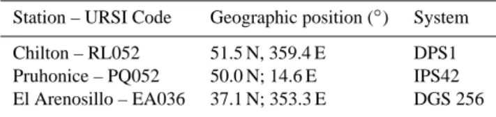
Table 1. List of the ground-ionosonde stations used in this study.
Station – URSI Code Geographic position (◦) System Chilton – RL052 51.5 N, 359.4 E DPS1 Pruhonice – PQ052 50.0 N; 14.6 E IPS42 El Arenosillo – EA036 37.1 N; 353.3 E DGS 256
GOES began its solar measurements in 1976 (Woods et al., 2004). Large fluxes of particles were sent to the Earth from 29 to 31 October 2003, and the magnetic field component parallel to the Earth’s rotation axis (Hp) dropped to −150 nT
twice, as recorded by the GOES-10 satellite. Moreover, the estimated planetary K-index (Kp) reached severe storm
levels for almost three days, the planetary Ap-index (Ap)
reached values as high as 400 nT and the Dst index dropped
twice below −340 nT (−349 nT on 29 October and −401 nT on 30 October). Despite the high values of the Interplan-etary Magnetic Field (IMF) as recorded by the Solar Wind Electron Proton Alpha Monitor instrument (SWEPAM) on the Advanced Composition Explorer (ACE), these were not unprecedented and a high magnetic field disturbance lasted only for a short time. Moreover, although the IMF proton density recorded by SWEPAM on ACE was uncertain for much of the highest solar wind speed (1850 km/s), the rel-atively low proton density led to a moderate dynamic pres-sure. The latter, together with a short-lived negative Bz
com-ponent of the IMF, were the reasons why the October 2003 event was not unusually geoeffective, as it was expected to be. However, an even larger geomagnetic storm with Dst
reaching −470 nT occurred 3 weeks later, on 20 November 2003 when the solar wind speed was only ∼750 km/s. Simi-lar storms were produced by the 15 July 2000 and 31 March 2001 solar events (Skoug et al., 2004).
The aim of this paper is to show and discuss some effects observed on the ionosphere from several European ionoson-des and Global Positioning System (GPS) stations during the November 2003 geomagnetic storm. A discussion of the Helio-Geophysical background for the November 2003 event is introduced. Taking into account the global extent of the great geomagnetic storms and the strong gradients involved, the simultaneously monitoring of a large ionospheric area is advantageous. The GPS data enables us to carry out electron concentration measurements along a slant signal path and to obtain Vertical Total Electron Content (VTEC) by sim-ple mathematical formalism. The availability of ionosonde data (with high vertical resolution) and ground GPS (with high spatial and temporal resolution) brings important in-formation for the study of the ionosphere. This is being exploited by different authors to better investigate the solar geomagnetic storms (see, for instance, Yin et al., 2004 and Liu et al., 2004, for Storm Imaging and Solar Flare stud-ies, respectively). In the case of GPS this is also impor-tant as well, from the practical point of view, because the augmentation systems, such as EGNOS in Europe, designed
for civil aviation navigation among others, can be affected (Hernandez-Pajares et al., 2005). Using both data types, ground-ionosonde and GPS, we can observe two distinct ef-fects on the mid-latitude ionosphere over the European Sec-tor: the generation of anomalous storm sporadic E layers (similar to auroral Es layers), probably formed by energetic
particle precipitation and with virtual heights of about 150– 200 km at latitudes as low as 37◦N, and the generation of two thin longitudinal belts of VTEC, one with enhanced VTEC and the other with depressed VTEC.
2 Data
The Helio-Geophysical background for the November 2003 event is obtained from several data sources. The IMF data are obtained from ACE MAG Level 2 data, and the Solar Wind velocity and density are obtained from ACE SWEPAM Level 2, both provided by the ACE Science Center (ASC) (http://www.srl.caltech.edu/ACE/ASC/). ACE orbits the L1 libration point, which is a point of Earth-Sun grav-itational equilibrium about 1.5 million km from the Earth and 148.5 million km from the Sun. With a semi-major axis of approximately 200 000 km the elliptical orbit affords ACE a prime view of the Sun and the galactic regions be-yond. Proton fluxes and the magnetic field component par-allel to the Earth’s rotation axis (Hp) at geostationary orbit
distance from the Earth are obtained from GOES-10 satel-lite data (longitude of 135◦W) at the Space Environment
Center (http://sec.noaa.gov/Data/). The geomagnetic activ-ity indices Ap and Dst are obtained from the International
Service of Geomagnetic Indices (ISIG) of the International Association of Geomagnetism and Aeronomy (IAGA) at http://www.cetp.ipsl.fr/∼isgi/homepag1.htm.
The effects on the Earth’s ionosphere during the November 2003 geomagnetic storm were observed from ground-based ionosonde and GPS data. Table 1 shows the ionosonde sta-tions involved in this study. Data from Pruhonice and El Arenosillo were supplied directly from each observatory and Chilton data were obtained via ftp from WDCC1 at RAL, ftp://wdcc1.bnsc.rl.ac.uk/.
Ground-based ionosonde offers high resolution data up to the ionospheric F region maximum electron density height hmF2, providing a vertical electron density profile (N (h)).
We computed the “true height” profiles of plasma frequency (fp) in the altitude range from 90 to 800 km for Chilton and
El Arenosillo ionograms. Note that fpis related to the
elec-tron density by the well-known expression N = 1
80.6f
2
p, (1)
where fpis expressed in Hzand N in m−3.
We used the standard “true height” inversion algorithm described by Huang and Reinisch (1996) to calculate the bottomside profiles, and the Reinisch and Huang (2001) algorithm has been used to calculate the topside profiles. The electron density profiles were obtained after operator-scaled ionograms were obtained by the DGS 256 and DPS4
sounders of El Arenosillo and Chilton, respectively, to ensure profile data quality and to avoid possible mistakes from the automatic scaling data recorded by the sounders.
To obtain good information above hmF2(up to 20 000 km
high), we used the ground Global Positioning System data to estimate accurately VTEC, with typical errors of a few TECUs (Hernandez-Pajares et al., 1999). Using data from the 928 available GPS stations in the Northern Hemisphere, a global map with high time resolution (10 min) showing the VTEC evolution in the Northern Hemisphere has been computed. An ionospheric tomographic voxel model was solved by running a Kalman filter feed with data from about 150 worldwide distributed GPS receivers belonging to the International GPS Service (IGS) network (see more details in Hernandez-Pajares et al., 2002). Afterwards, to reach the maximum available resolution, the overall available GPS receiver measurements in the Northern Hemisphere (900+) were transformed to STEC by aligning the ionospheric car-rier phase observable to the first tomographic determination.
3 Background
The Helio-Geophysical conditions raised during the 19– 21 November 2003 event are depicted in Fig. 1. This fig-ure shows the solar wind (SW) background at 1.5 million km from the Earth (plots a, b and c). We observe that the Bzcomponent of the IMF displays large variability, starting
at about 07:30 UT on 20 November. It dropped rapidly to strongly negative values (reaching a minimum value of about −50 nT), and negative values of Bz are long-lasting (from
about 11:00 to 23:00 UT on 20 November). As first sug-gested by Dungey (1961), the Bzorientation has an
impor-tant influence on the magnetosphere and high-latitude iono-sphere, and the more negative Bzis, the more important are
the effects on the ionosphere (Davis et al., 1997). Moreover, an abrupt increase in the SW velocity (from about 450 to 750 km/s) and in the SW density (by factor 3) is noticed at about 07:30 UT on 20 November. These enhancements last for about 4 h, and afterwards, the SW velocity returns to typ-ical values of about 500 km/s, whereas SW density displays three additional bursts, the largest one occurring from 15:00 to 21:00 UT on 20 November. These facts provide a sig-nificant enhancement of the dynamic pressure of the SW on the magnetosphere and may leave satellites unprotected, thus causing damage.
This fact is observed from GOES-10 data. Plot (d) of Fig. 1 shows how the Hpat the GOES position dropped
sud-denly to −250 nT after a relatively stable condition. The strong negative values of Hp last for several hours, from
16:30 to 22:00 UT on 20 November, approximately. Plot (e) of Fig. 1 shows a dramatic increase in the proton flux (by a factor of 10) at about 12:00 UT on 20 November. Al-most simultaneously, severe storm levels of geomagnetic ac-tivity were recorded (plots (f) and (g) of Fig. 1). The Ap
index reached 300 nT (Kp=8+) between the 3-h intervals
from 16:30 to 19:30 UT on 20 November, and the Dst
in-Fig. 1. Plot (a) shows the IMF Bz component (GSM coordinate
system), plot (b) shows solar wind velocity, and plot (c) shows the solar wind density; all of them recorded by the ACE satellite. Plot
(d) shows the magnetic field component parallel to the Earth’s
rota-tion axis (Hp), and plot (e) shows the proton flux (on red for proton
with energy 4–9 MeV, on blue for 9–15 MeV, and on yellow for 15– 40 MeV); all of them recorded by GOES-10. Plots (f) and (g) show the 3-h Ap and hourly Dst geomagnetic activity indices,
respec-tively (obtained from ISIG – IAGA).
dex dropped to superstorm values of about −470 nT at 1900 on 20 November. With the above background, strong iono-spheric effects were expected.
3030 E. Blanch et al.: November 2003 event: effects on the Earth’s ionosphere
Fig. 2. Examples of ionograms obtained in Chilton (left plots) and
El Arenosillo (right plots) at the indicated time. The ionograms are 2-D plots of the reflection altitude (virtual height) for a vertically emitted pulse at a given radio frequency (plasma frequency). Red to bluish dots correspond to the reflection points of the Ordinary beam and green dots correspond to the Extraordinary beam. The black lines following the trace of the Ordinary beam of the regular layers (E and F ) have been used to obtain the “true height” electron den-sity profiles (blue line) by the inversion algorithms, as described in Sect. 2. The grey lines following the Ordinary beam of the “anoma-lous storm Es” layers have been used to obtain the contribution to
the electron density profiles (red line) of these anomalous layers.
Fig. 3. Examples of ionograms recorded in Chilton at the indicated
time, showing different types of “anomalous storm Es” layers.
4 Observation
The effects on the ionosphere of the strong geomagnetic storm which occurred on 20 November were observed at the three ionospheric stations listed in Table 1. Figure 2 shows some ionograms recorded at Chilton and El Arenosillo, showing distinct features of ionospheric effects caused by the 20 November event. Although not shown here, a significant increase in the electron density in the F2layer has been
ob-Fig. 4. As in ob-Fig. 3, but for Pruhonice. Notice that the sounder
IPS42 from Pruhonice is not able to distinguish between the ordi-nary and extraordiordi-nary beams in the ionograms.
served for both Chilton and Pruhonice stations at about noon, followed by a short-lasting decrease in the electron density and the later appearance of the well-developed anomalous storm Es layers. Above Chilton, the critical frequency of the
F2 layer, f0F2, started to become smaller and the F2layer
electron density peak altitude, hmF2, increased rapidly after
15:00 UT. The anomalous storm Es layer, developed at the
height of 110 km, was first recorded on Chilton ionograms at 16:40 UT, with a corresponding density much larger than under quiet conditions. Echo patterns showed a flat, slowly rising, lower edge with a rapidly changing stratified struc-ture. The spreading ranged over several hundred kilometres in virtual height. These anomalous storm Eslayers were
ex-hibited for several hours, until 22:30 UT, approximately, and it hid the F -region evolution (blanketing effect). The left plots of Figs. 2 and 3 show some of the ionograms repre-senting the above facts. Quite similar ionospheric responses to storm-induced disturbances, as the ones observed above Chilton station, were observed above the Pruhonice observa-tory. At 16:55 UT a thick anomalous Es layer appeared and
it lasted for several hours (Fig. 4). Comparing with Chilton, the anomalous storm Es layer over Pruhonice was observed
at higher altitudes (from 120 to 150 km) and also hid the F -region behaviour most of the time until midnight. A posi-tive storm effect on the ionospheric F -region electron den-sity above the El Arenosillo station was observed at about 09:00 UT (to be discussed later in Fig. 5). From 18:00 UT to 23:00 UT, El Arenosillo recorded a significant increase in f0F2and hmF2, and a strong spread F condition was clearly
observed, lasting practically the whole night of 20 Novem-ber. We observed that the anomalous storm Es layers also
appeared above this mid-low latitude station, although not as strong as over the other two stations, and it did not hide the
F region on the ionograms (right ionograms in Fig. 2). This unusual sporadic Eslayer persisted only three hours in the El
Arenosillo ionograms and it was able to observe the time re-sponse of the F -region from the ionograms. The occurrence of this unusual storm Es layer is very rare at mid-latitude
stations.
The thick “night-time E” layers usually occur in auroral regions at times of geomagnetic disturbances, as discussed by King (1962). According to Brown and Wynne (1967), this can also be observed at mid-latitudes in association with auroral activity. The phenomenon of the anomalous storm Es
is attributed to particle precipitation during ionospheric dis-turbances and to electromagnetic drift produced by the storm electric field system. The evening and night-time ionograms recorded at Chilton and Pruhonice during 20 November 2003 show the presence of such an anomalous storm Es, and some
of them remind us of the shape of the auroral Es layers or
particle Es layers (Figs. 3 and 4). According to the
Re-port UAG23A of the World Data Center A (1978), as well as its revised edition (1986), the anomalous storm Es layers
observed in the Chilton ionograms at 16:50 and 17:00 UT (Fig. 3) and at 17:40 UT (Fig. 2) can be classified as standard type r (retardation), with a slightly rising edge and spreaded trace. Therefore, it can also be interpreted that the particle layer is blanketed by the r type Es. The anomalous storm
Es layer, which is present in the Chilton ionograms recorded
after 20:00 UT, seems to be closer to the standard type a (au-roral) than type r Es layers.
The particle Eslayer (type k) is a thick layer, which is
pro-duced by the participating particles moving into the lower at-mosphere during ionospheric disturbances, showing a larger virtual height than that of the normal Es(up to 170 km). This
is often observed in the night-time with a type r or type a trace at high latitudes. However, the anomalous storm Es
layers observed in the higher-middle latitude station Pruhon-ice ionograms, from 16:55 to 17:10 UT (Fig. 4), and in the lower-middle latitude station El Arenosillo ionograms, from 18:00 to 19:00 UT (Fig. 2), can also be classified as type k. The anomalous Es layer recorded in the later Pruhonice
ionograms, starting at 20:00 UT, seems to be closer to a type a Es, exhibited together with a r type trace (Fig. 4). The
occurrence of the auroral Es layers over middle to lower
lat-itudes appears to be a superstorm phenomenon produced by energetic particle precipitation.
The positive and negative effects are difficult to detect us-ing only ground-ionosonde data due to several phenomena, such as absorption and F -region blanketing by sporadic E layers (which occurred above Chilton and Pruhonice). A de-tail of the latter effect may be seen in Fig. 5 for the Chilton station. However, we are able to see a positive storm ef-fect above the El Arenosillo station. In Fig. 5 we compare the evolution of the plasma frequency as a function of time and altitude above Chilton and El Arenosillo for perturbed day 20 November 2003 with that of the previous day. It can clearly be seen from Fig. 5 that the anomalous storm Es
lay-ers hide the information of the F region in the Chilton iono-grams. This is why the contour plot of Fig. 5,
correspond-Fig. 5. Time-altitude cross-section plots of plasma frequency above
Chilton (top plots) and El Arenosillo (bottom plots) on the indicated days. The colour scale at the bottom indicates the different levels of plasma frequency.
ing to Chilton for the perturbed day, only accounts for the contribution of the “anomalous storm Es” layers during the
time interval 16:50–22:30 UT, approximately. There are no F-region profiles available for that time interval because of a blanketing effect of the “anomalous storm Es” layers, as
already discussed from Fig. 2. However, direct comparison of plasma frequency evolution above El Arenosillo between pre-storm and the storm day, allows us to observe the fol-lowing facts. The daily variation of 20 November behaves quite similar to that observed for the previous day, up to early afternoon, despite the larger density around midday. In the early evening, an enhancement of plasma frequency (by a factor 3 to 4) is clearly stated during the initial phase of the storm (from 18:00 UT onwards). Simultaneously, the F re-gion is lifted and one can see that it also spreads in altitude. This may originate from an enhancement of the equatorward meridional component of the neutral wind, as compared with the previous day and from an enhancement of the plasma temperature, both caused by the geomagnetic storm. The latter facts can explain the lifting and widening of the F re-gion and the observed electron density enhancement, as well (Danilov, 2001; Pr¨olls, 2004).
In order to avoid all the absorption and blanketing phe-nomena on the ionograms and to have additional infor-mation about the ionosphere, we use GPS ground data. The UPC/gAGE computed the VTEC evolution (every 10 min) to study the ionospheric effects caused by the
3032 E. Blanch et al.: November 2003 event: effects on the Earth’s ionosphere
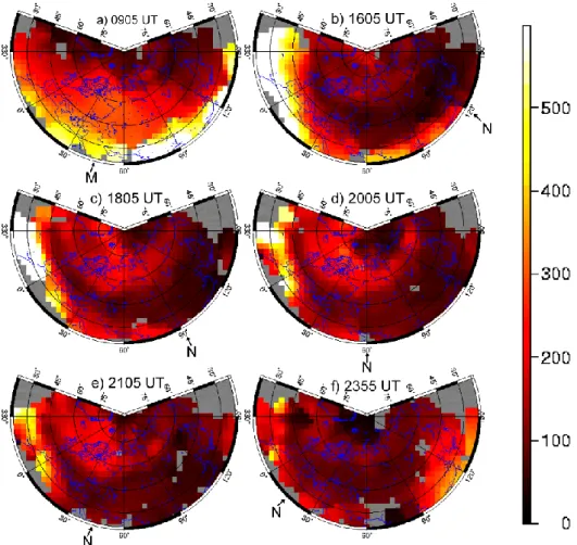
Fig. 6. Two-dimensional maps showing the evolution of VTEC on 20 November 2003 in the Euro-Asiatic Sector. The geographical parallels
are plotted every 15 degrees from the geographical North Pole, and corresponding meridians plotted every 30 deg. Arrows indicate the local noon (M) or local mid-night (N). The color scale indicates the levels of VTEC in units of 0.1 TECU (1015m−2). The grey regions are not covered by GPS receivers. First snapshot (a) shows the VTEC values at about the storm onset. Snapshot (b) shows VTEC at the end of the initial phase of the storm. Snapshots (c), (d), and (e) show VTEC at the main phase. Snapshot (f) shows VTEC at the early recovery phase of the storm.
20 November 2003 event in the Northern Hemisphere from the overall permanent receivers (900+). In Fig. 6 we present some of the snapshots where the storm effects on VTEC can be seen. We focus our attention on the European sector in the evening, due to the availability of two data types, and due to the very dramatic effects produced. From Fig. 6 one observes that under quiet conditions (snapshot 6a), VTEC values are lower at the nightside and at high latitudes. VTEC starts to increase around the auroral oval down to around 60◦N at the initial phase of the storm (snapshot 6b). Around 18:00– 21:00 UT (snapshots c, d, e, and even f), one can notice the existence of a thin latitudinal belt between 55◦−45◦N,
with lower VTEC values than those at the higher latitude, extending into the longitude sector 350◦–30◦E, this
latitu-dinal belt being wider into the longitude sector 50◦–120◦E. In addition, an enhanced VTEC is clearly stated on the lat-itudinal belt between 45◦−30◦N during the evening hours of 20 November, into the longitude sector 330◦–60◦E, ap-proximately. This effect was expected to be observed from the ground ionosonde data; but the anomalous storm Es
lay-ers hid the F -region evolution above Chilton and Pruhonice. However, from ionograms depicted in Fig. 2, one can see that the F -region electron density tends to depress strongly for Chilton. Although not shown here, Pruhonice had measure-ments at 5-min sampling, and some of the ionograms allow one to observe the F region, indicating very low densities. Direct comparison between Figs. 2 to 6 supports the fact that in the European sector, in the evening, the storm caused a thin latitudinal belt (55◦–45◦N) with depressed electron densities in the F region during the main phase of the storm (negative effect) and a positive effect in the latitudinal belt from 45◦to 30◦N. Moreover, we clearly observe from Fig. 6 that the
au-roral oval expands from 60◦N at the initial phase of the storm
(snapshot b) to latitudes as low as 45◦N for the evening
5 Summary and discussion
Two periods of a suddenly enhanced solar activity in October and November 2003 resulted in two strong geomagnetic and ionospheric storms. The effects of both events were danger-ous for satellite equipment and influenced many communi-cation, navigation (GPS, GNNS) and technological systems. It is very interesting that the smallest storm produced a more dramatic effect on the Earth’s ionosphere in the mid-latitude European sector. These rare types of effects are practically not predictable at this time.
Investigations of the mid-latitude sporadic E layer carried out into the framework of COST 271 Action (http://www. cost271.rl.ac.uk/) have been briefly described by Bencze et al. (2004). In general, the frequency parameters of sporadic Eare considered as a quantity proportional to the mean ion-density of “patches” of increased ion ion-density in the layer, and its temporal variation may indicate the mean periodic-ity of ion densperiodic-ity changes. The “storm sporadic E” is the most striking phenomenon in the ionospheric E region. Usu-ally it occurs at moderately high latitudes ranging from 78◦to 68◦and expands toward lower latitudes during disturbances (Rishbeth and Garriott, 1969). Electron density distribution at the heights of the storm sporadic E layer has been stud-ied by Thomas (1962) and is related to auroral oval phenom-ena. Ionospheric behavior, such as storm sporadic E, is at-tributed to intense, rapidly fluctuating and spatially limited “splashes” of precipitated particles.
During the November 2003 geomagnetic storm, the first effect we observed is the generation of “anomalous storm Es” layers, whose strength and blanketing intensity depend
on latitude. The latter properties are larger at higher latitude. These anomalous layers appear down to mid-low latitude sta-tions like El Arenosillo, but the occurrence was shorter com-pared to the higher latitude stations of Pruhonice and Chilton, due to the lower latitude of El Arenosillo. The height and shape of these “anomalous storm Es” layers are typical for
layers formed by energetic particle precipitation. The exis-tence of this particle layer does not permit one to follow the F region response to the geomagnetic storm using ground ionosonde data in the higher latitude stations. However, the VTEC maps obtained from ground GPS receivers allow to follow the global response of the ionosphere, but we have no details on the vertical structure. Therefore, the use of both of these data types allows us to observe more than one dis-tinct effect of the November storm over mid-latitude Euro-pean sector.
The second effect we observe is the generation of two dis-tinct latitudinal belts, in the European evening sector. Dur-ing the main phase of the storm, a thin latitudinal belt (55◦– 45◦N) with depressed VTEC (negative effect) and an ad-ditional latitudinal belt (45◦–30◦N) with enhanced VTEC (positive effect) are observed. The latter effect, the so-called negative storm effect, can be explained by changes in compo-sition caused by the storm, or it could be linked to the equato-ward expansion of the main ionospheric trough caused by the storm. General circulation models shows realistic changes in
neutral composition that account for negative storm effects (Fuller-Rowell et al., 1991). In addition, empirical models (Araujo-Pradere et al., 2004) show the dependence of the estimated variability of f0F2 on latitude, season and
geo-magnetic activity. They assessed dominant negative storm effects in the latitude range 80◦–40◦N during winter and the intermediate seasons, and dominant positive storm effects in the latitude range 40◦–20◦N. Moreover, Burns et al. (1995) demonstrated that geomagnetic storms drive large enhance-ments of O/N2 in a limited latitudinal region of the winter
hemisphere in the evening sector. Such an effect would pro-duce a depressed loss rate of electron density in the above limited region, leading to an enhancement of the electron density (Rishbeth and Barron, 1960). This fact of enhanced electron density in a limited latitudinal belt is just the one we observed from the VTEC maps and it can be explained by the facts described in Burns et al. (1995). As discussed by Burns et al. (1995) as well, such enhancements would be caused by large gravity wave, but only if its duration is lower than a few hours. Despite the enhancement of VTEC, we observe a long-lasting effect, persistent for more than 10 h after onset. Therefore, we believe that the changes in composition gener-ated by the storm are the cause of the VTEC enhancements observed in the mid-latitude evening sector. Moreover, an ad-ditional belt of depressed VTEC has been noticed. Regarding the latter, the electric fields and particle populations which characterize the auroral region expand equatorward during geomagnetic storms, and their effects can be perceived at sub-auroral latitudes. Intense convection electric fields ap-pear in the expanded auroral oval (Yeh et al., 1991) and are responsible for density depletion and ionospheric trough for-mation due to the effects of enhanced recombination (Schunk et al., 1976).
Acknowledgements. This paper is based on the results presented at the First European Space Weather Week, Noordwijk, December 2004, whose participation was funded by COST Action 724. The authors are grateful to El Arenosillo, Pruhonice and Chilton obser-vatories, as far as to IGS for the data availability. The authors would like to thank the ACE SWEPAM instrument team and the ACE Sci-ence Center for providing the ACE data, and to the information from the Space Environment Center, Boulder, CO, National Oceanic and Atmospheric Administration (NOAA), US Dept. of Commerce. This work has been partially supported by the Spanish project REN2003-08376-C02-02. The work of J. Boˇska and D. Bureˇsov´a has been partially supported by the Grant of the Academy of Sci-ences of the Czech Republic S300120506. The work of last au-thor has been partially supported by Spanish projects PETRI95-07522.OP.01 and ESP2004-045682-C02-01.
Topical Editor M. Pinnock thanks I. Kutiev and another referee for their help in evaluating this paper.
3034 E. Blanch et al.: November 2003 event: effects on the Earth’s ionosphere
References
Araujo-Pradere, E. A., Fuller-Rowell, T. J., and Bilitza, D.: Iono-spheric variability for quiet and perturbed conditions, Adv. Space Res., 34, 9, 1914–1921, 2004.
Bencze, P., Buresova, D., Lastovicka, J., and Marcz, F.: Behavior of the F1-region, and Es and spread-F phenomena at European
middle latitudes, particularly under geomagnetic conditions, An-nals of Geophysics (Rome, Italy), 47, 2/3, 1131–1143, 2004. Brown, G. M. and Wynne, R.: Solar daily disturbance variations in
the lower ionosphere, Planet. Space Sci., 15, 1677–1686, 1967. Buonsanto, M. J.: Ionospheric Storms – A review, Space Sci. Rev.,
88, 563–601, 1999.
Burns, A. G., Killeen, T. L., and Carignan, G. R.: Large enhance-ments in the O/N2 ratio in the evening sector of the winter hemisphere during geomagnetic storms, J. Geophys. Res., 100, 14 661–14 671, 1995.
Danilov, A. D.: F2-region response to geomagnetic disturbances, J. Atmos. Sol.-Terr. Phys., 63, 441–449, 2001.
Davis, C. J., Wild, M. N., Lockwood, M., and Tulunay, Y. K.: Iono-spheric and geomagnetic responses to changes in IMF Bz: a su-perposed epoch study, Ann. Geophys., 15, 217–230, 1997,
SRef-ID: 1432-0576/ag/1997-15-217.
Dungey, J.W.: Interplanetary magnetic field and the auroral zones, Phys. Rev. Lett., 6, 47–48, 1961.
Fuller-Rowell, T. J., Codrescu, M. V., Moffett, R. J., and Quegan, S.: Response of the thermosphere and ionosphere to geomagnetic storms, J. Geophys. Res., 99, 3893–3914, 1994.
Fuller-Rowell, T. J., Rees, D., Risbeth, H., Burns, A. G., Killeen, T. L., and Roble, R. G.: The composition change theory of F-region storms, J. Atmos. Terr. Phys., 53, 797–815, 1991.
Hernandez-Pajares, M., Juan, J. M., and Sanz, J.: New approaches in global ionospheric determination using ground GPS data, J. Atmos. Sol.-Terr. Phys., 61, 1237–1247, 1999.
Hernandez-Pajares, M., Juan, J. M., and Sanz, J.: Improving the real-time ionospheric determination from GPS sites at Very Long Distances over the Equator, J. Geophys. Res., 107, 1296–1305, 2002.
Hernandez-Pajares, M., Juan, J. M., Sanz, J., Farnworth, R., and Soley, S.: EGNOS Test Bed Ionospheric corrections under the October and November 2003 Storms, IEEE Transactions on Geo-science and Remote Sensing, 43, 10, 2283–2293, 2005. Huang, X. and Reinisch, B. W.: Vertical electron density profiles
from the Digisonde network, Adv. Space Res., 18, 6, 21–29, 1996.
King, G. A. M.: The night E-layer, in: “Ionospheric Sporadic E”, edited by: Smith, E. K. and Matsushita, S., 219–231, Pergamon Press, Oxford, UK, 1962.
Lastovicka, J.: Monitoring and forecasting of ionospheric space weather – effects of geomagnetic storms, J. Atmos. Sol.-Terr. Phys., 64, 697–705, 2002.
Liu, J. Y., Lin, C. H., Tsai, H. F., and Liou, Y. A.: Iono-spheric solar flare effects monitored by the ground-based GPS re-ceivers: Theory and observation, J. Geophys. Res., 109, A01307, doi:10.1029/2003JA009931, 2004.
Mansilla, G. A.: Mid-latitude ionospheric effects of a great geomag-netic storm, J. Atmos. Sol.-Terr. Phys., 66, 1085–1091, 2004. Ondoh, T. and Marubashi, K.: Overview of the science of the space
environment, in: Science of space environment, edited by: On-doh, T. and Marubashi, K., 1–27, Ohmsha, Ltd., Tokyo, Japan, 2001.
Pr¨olss, G. W.: Physics of the Earths Space Environment, Springer-Verlag, Berlin Heidelberg, Germany, 2004.
Reinisch, B. W. and Huang, X.: Deducing topside profiles and total electron content form bottomside ionograms, Adv. Space Res., 27, 23–30, 2001.
Rishbeth, H. and Barron, D. W.: Equilibrium electron distributions in the ionospheric F2-layer, J. Atmos. Terr. Phys., 18, 234–252, 1960.
Rishbeth, H. and Garriott, O. K.: Introduction to ionospheric physics, Academic Press, New York and London, 1969. Schunk, R. W., Banks, P. M., and Raitt, W. J.: Effects of
elec-tric fields and other processes upon the nighttime high-latitude
Flayer, J. Geophys. Res., 81, 3271–3282, 1976.
Skoug, R. M., Gosling, J. T., Steinberg, J. T., McComas, D. J., Smith, C. W., Ness, N. F., Hu, Q., and Burlaga, F. L.: Extremely high speed solar wind: 29-30 October 2003, J. Geophys. Res., 109, A09102, doi:10.1029/2004JA010494, 2004.
Thomas, L.: The distribution of dense Esionisation at high latitudes
J. Atmos. Terr. Phys., 24, 643–658, 1962.
Thomson, N. R., Rodger, C. J., and Dowden, R. L.: Ionosphere gives size of greatest solar flare, Geophys. Res. Lett., 31, L06803, doi:10.1029/2003GL019345, 2004.
U.R.S.I.: Handbook of ionogram interpretation and reduction, edited by: Piggott, W. R. and Rawer, K., WDC A, National Academy of Sciences, Washington, D. C., USA, 1978.
U.R.S.I.: Manual of ionogram scaling, Revised Edition, edited by: Wakai, N., Ohyama, H., and Koizumi, T., Radio Research Labo-ratory, Japan, 1986.
Woods, T. N., Eparvier, F. G., Fontenla, J., Harder, J., Kopp, G., Mc-Clintock, W. E., Rottman, G., Smiley, B., and Snow, M.: Solar ir-radiance variability during the October 2003 solar storm period, Geophys. Res. Lett., 31, L10802, doi:10.1029/2004GL019571, 2004.
Yeh, H.-C., Foster, J. C., Rich, F. J., and Swieder, W.: Storm-time field penetration observed at mid-latitude, J. Geophys. Res., 96, 5707–5721, 1991.
Yin, P., Mitchell, C. N., Spencer, P. S. J., and Foster, J. C.: Iono-spheric electron concentration imaging using GPS over the USA during the storm of July 2000, Geophys. Res. Lett., 31(L12806), doi:10.1029/2004GL019899, 2004.