HAL Id: hal-02326278
https://hal.archives-ouvertes.fr/hal-02326278
Submitted on 22 Oct 2019
HAL is a multi-disciplinary open access
archive for the deposit and dissemination of sci-entific research documents, whether they are pub-lished or not. The documents may come from teaching and research institutions in France or abroad, or from public or private research centers.
L’archive ouverte pluridisciplinaire HAL, est destinée au dépôt et à la diffusion de documents scientifiques de niveau recherche, publiés ou non, émanant des établissements d’enseignement et de recherche français ou étrangers, des laboratoires publics ou privés.
F. Taccogna, Laurent Garrigues
To cite this version:
F. Taccogna, Laurent Garrigues. Latest progress in Hall thrusters plasma modelling. Reviews of Modern Plasma Physics, Springer Singapore, 2019, 3 (1), �10.1007/s41614-019-0033-1�. �hal-02326278�
________________________________________________________________________________ Reviews of Modern Plasma Physics (2019) …
https://doi.org/.... 1 REVIEW PAPER
Latest Progress in Hall Thrusters Plasma Modelling
F. Taccogna1 L. Garrigues2
Received: ? / Accepted: ?
Abstract
In the last thirty years, numerical models have revealed different physical mechanisms involved in the Hall thruster functioning leading to a bridge between analytical prediction / empirical intuition and experiments. For this reason, modeling effort is continuously increasing in the domain of Hall Thrusters. Two basic approaches exist: one based on fluid/hybrid simulation where the distribution of electrons is assumed Maxwellian and the plasma inside the thruster, considered as quasineutral, is described with macroscopic quantities (density, velocity and energy); the second approach is based on kinetic description for charged particles where no approximation is made for the distribution of particles.
Fluid or hybrid approaches offer the advantage of demanding low run times and computational resources. They are very useful to perform parametric studies but actually the anomalous phenomena responsible for electron transport across the magnetic field barrier have not been self-consistently modeled. Kinetic approach is able to better capture phenomena originating on the Debye scale length like the lateral sheaths, ExB electron drift instability, important to explain the anomalous electron transport, but it requires very long run times. For this latter, the progress in computer science offers the advantage to describe conditions more and more close to the thruster operation.
In this review, we will present the two approaches emphasizing on numerical schemes used with assumptions and approximations and on main results obtained. Future directions on the Hall thruster modeling will finally outlined.
Keywords Hall Thruster · Particle-in-Cell · Plasma sheath · Secondary electron emission · Electron
cyclotron drift instability
F. Taccogna
Extended author information available on the last page of the article Published online: ?
________________________________________________________________________________
1 Introduction
To move and/or control the motion of satellites around Earth's orbit or spacecrafts for Space trips, a propulsion system must be used to achieve the mission by exerting a force called thrust under the ejection of matter (action-reaction principle). The success of electric propulsion utilization is based on the ability to eject a high-speed propellant and mass economy induced at launch to realize such missions. For a large overview and state-of-art of the electric propulsion topic, the reader can refer to textbooks of Jahn (2006), Turner (2009), Goebel and Katz (2008), to review articles of Ahedo (2011), Garrigues and Coche (2011), Mazouffre (2016), Levchenko et al. (2018), and to recent special issues of IEEE Transactions on Plasma Sciences, vol. 43(1) (2015) and Plasma Sources Science and Technology, vol. 27 (2018).
Robert Jahn defining the electric propulsion as the acceleration of gases for propulsion by electrical heating and/or electric and magnetic body forces, electrical thrusters have been classified in three main categories.
- Electrothermal thrusters are based on same principles than chemical thrusters where the thrust is the result of a hot gas expansion through a nozzle used to convert thermal energy to kinetic energy, expect that gas heating is achieved through the means of an arc (arcjet) or a resistance (electrojet). - In electromagnetic thrusters, a propellant gas is ionized. The thrust is produced by the acceleration of charged particles under the Lorentz force that is a combination of applied electric and self-induced magnetic fields resulting from a high discharge current maintained in the plasma.
- Electrostatic thrusters are also based on the ionization of a propellant gas but the thrust is the result of the acceleration of positive ions by an imposed direct-current electric field. Injection of electrons ensured by a neutralizer is necessary to maintain a zero net-current beam. Gridded ion engines are one of the oldest electrostatic thrusters. It consists of two separate stages, an ionization chamber where the plasma is generated by means of direct-current with multipole magnetic field ring-cusp (Kaufman-type source), radio-frequency or microwave fields, and an acceleration stage with a system of polarized grids to accelerate ions at the desired velocity. The main drawback of such engine is due to space charge formed upstream of the grid system that acts as a limiting factor in term of the ion current density extracted and thrust by units of surface (Child-Langmuir law). New missions for electric propulsion, requiring one unique type of engines to be able to ensure high thrust level during orbit transfer, cannot be currently achieved with compact gridded ion engines. A particular concept of electrostatic propulsion is represented by Hall Thruster (HT). It is based on the application of a magnetic field barrier perpendicular to the direction of the discharge current. In such a way, the electron conductivity locally drops leading to the penetration of the direct-current electric field within the plasma (Boeuf 2017). The axial electric field resulting from the potential drop between anode and cathode electrodes serves to ignite and maintain the plasma by heating electrons and to accelerate ions to furnish the thrust, without space charge limitation. The discharge takes place inside a coaxial channel made in ceramics, generally a boron-nitride with silica compounds, BN-SiO2 (see Figs. 1 for a schematic and the operations of a 20 kW-class engine).
From now on we will always use the cylindrical coordinate system to indicate the various directions The gas propellant (usually heavy noble gases) is impeded at the rear of the channel, through a metallic anode plane. An external cathode serves as electron source whose current is split in two: one fraction corresponding to ~ 20 % of the discharge current is going inward of the channel and after being heated by the electric field ionizes the neutral gas, the rest neutralizes the ion beam ejected from the channel. The discharge current at the anode (~ 4A for a kW-class Hall thruster) is carried by electrons coming from the external cathode source and resulting from the multiplication
________________________________________________________________________________ in the channel during the gas ionization (fixing the ion current strength produced). The magnetic field whose direction is mainly radial and strength maximum at the exhaust of the channel is established thanks to a system of inner and outer coils and a magnetic circuit made in iron-based materials. The magnetic field strength ~ 100 G is chosen to only confine electrons keeping ions un-magnetized. A Hall current in the azimuthal E×B direction is not interrupted because of the cylindrical symmetry increasing the residence time of the electrons inside the channel giving rise to ionize ~ 90 % of the neutral flux injected. The name of the thruster comes from the azimuthal Hall electron current, while the name of closed electron drift thruster is preferred in the Russian literature.
(a) (b)
Fig. 1 (a) Schematic of Hall thruster, (b) PPS®-20K ML mounted with the centered cathode operating at different
power levels (photo credit: Safran-Snecma).
This review paper is focused on the modeling of HTs and is split in two main parts.
In Sect. 2, fluid/hybrid-based models and main features of the thruster discharge obtained with are detailed. Supported by the existence of an electric field penetrating inside the bulk plasma, the modeling of sheaths becomes un-essential (and can be treated analytically separately), and the hypothesis of quasi-neutrality is appropriated. It offers the advantage of not resolving Debye length and plasma frequency alleviating constraints on timestep and grid-spacing. Low computational cost makes possible parametric studies about the influence of magnetic field, discharge voltage and mass flow rate on thruster operation. In Sect. 2.1, fundamental equations are recalled and their implementations in the context of HT especially for the fluid treatment of strongly magnetized electrons are depicted. Sect. 2.2 is focused on the method to obtain the electric potential profile in quasi-neutral models and the encountered difficulties linked to an almost free transport of electrons along magnetic field lines contrary to the resistive cross-magnetic field transport. Analytical sheaths including secondary electron emission (SEE) under high-energy electron impacts on ceramic walls are treated in Sect. 2.3. The role of non-collisional phenomena that controls cross-magnetic field transport of electrons is crucial and cannot be captured in fluid/hybrid-based models for the simple reason that the azimuthal direction that is the siege of field fluctuations and induced transport is not described (see Sect. 3). Anomalous electron collision frequencies using empirical laws have consequently been introduced in electron transport equations (the different phenomena invoked are gathered in Sect. 2.4). Quantitative information about anomalous transport can also been extracted from measurements. An attempt to extract information from fully kinetic PIC simulations to self-consistently capture anomalous transport through the resolution of a wave equation is also discussed in Sect. 2.4. Even if fluid/hybrid models are not fully predictive, almost qualitatively, they are able to explain the complex operation of HTs, this is illustrated in the rest of that part. Sec. 2.5 gives a clear understanding of the thruster working and how the overlap between ionization and
inner coil
cathode
gas injection outer coil anode channel walls magnetic circuit E B E × B - +
-________________________________________________________________________________ acceleration regions are responsible for channel wall erosion and reduced thruster lifespan. Different operating regimes and the role of the type of ceramics are highlighted in Sect. 2.6. In Sect. 2.7, one example of utilization of fluid/hybrid-based models to predict channel wall erosion is detailed. One objective is to increase thruster lifetime and one possible way is to reduce radial electric field and sheath potential drop close to channel exhaust. After back and forth between simulations and experiments and after a deep analysis of plasma properties, one magnetic field topology called magnetic shielded configuration has been proposed and validated, this is detailed in Sect. 2.8.
Sect. 3 deals with the kinetic treatment of electrons. It is a fundamental aspect of HTs due to weak collisionality, anisotropy and strong SEE from the two lateral walls. The deviation from the equilibrium distribution can have an important impact on macroscopic quantities, like ionization efficiency, wall losses and transport coefficients. It can also drives microscopic instabilities leading to fluctuations in all the three directions at the expense of a thruster efficiency reduction. In Sect. 3.1 the models based on the direct solution of the electron Boltzmann equation will be presented. They shows the importance of the ExB configuration and electron-wall interaction. From Sect. 3.2 to Sect. 3.5 the different fully kinetic Particle-in-Cell (PIC) models developed for HTs will discussed. Sect. 3.2 presents one-dimensional radial models focusing on the importance of the lateral sheath regimes, electron-wall interaction and cylindrical geometry on the plasma dynamics in the acceleration region of the HT discharge channel. Sect. 3.3 presents the extension of radial models to include the axial coordinate. This leads to 2D axisymmetric models that give a quite complete representation (some time including also part of the plume region) of the HT functioning. Due to this completeness this class of models are often used to investigate particular magnetic field configuration and to assess the ion wall erosion. The plasma behavior along the azimuthal direction is presented in Sect. 3.4 where one-dimensional and the two two-dimensional (in combination with the axial and radial direction, respectively) models are presented. All results obtained have highlighted the importance of ExB drift instability to induce azimuthal fluctuations but also the limitation of low-dimensional models and the strong coupling among the different coordinates. The few fully kinetic three-dimensional attempts have finally been reported in Sect. 3.5. Kinetic effects can also be important in the plume region and in particular in the region close to the HT exit plane. Sect. 3.6 deals with some numerical approaches able to handle this problem. Finally, Sect. 3.7 is dedicated to the presentation of zero-dimensional kinetic models, such as global and collisional-radiative models. Summary and final evaluations and suggestions are reported in Sect. 4.
2 Fluid/hybrid models of channel and near field regions
In this section we focus on fluid/hybrid models of Hall thrusters and its applications to model the thruster operations.
2.1 Principles of fluid and hybrid approaches
Different types of models have been developed, starting from one-dimensional model along the axial direction inside the channel in the late 1990s, with an extension to the near field region where the magnetic field is still large, in the following years. At the same time, one-dimensional models along the radial direction have been used to simulate the effect of SEE under the impact of high-energy electrons on ceramic walls of the channel on plasma properties. Two-dimensional models that account for axial and radial directions most of time including channel and near field regions have been developed at the beginning of 2000s to better capture plasma properties and expansion. More recently, a two-dimensional model along the axial and azimuthal directions has been proposed. A list of models is given Tab. I. Developed models are fully fluid or hybrid when electrons are treated as a fluid and heavy species (ions and neutrals) with a kinetic description.
________________________________________________________________________________
Authors/References Model type SEE Transient Electric
Potential Regions
Boeuf and Garrigues (1998) 1D (z) hybrid No Yes QN Channel Ashkenazy et al. (1999) 1D (z) hybrid No No QN Channel Morozov and Savelyev (2000a) 1D (z) hybrid No Yes QN Channel Keidar et al. (2001) 1D (r) fluid Yes No Poisson Channel Ahedo et al. (2002) 1D (z) hybrid No No QN Channel/
Near field Roy and Pandey (2002) 1D (z) fluid Yes Yes QN Channel Ahedo (2002) 1D (r) fluid Yes No Poisson Channel Ahedo et al. (2003) 1D (z) hybrid Yes No QN Channel/
Near field Barral et al. (2003) 1D (z) fluid Yes Yes QN Channel Hara et al. (2012) 1D (z) hybrid No No QN Channel Komurasaki and Arakawa (1995) 2D (z,r) hybrid No No QN Channel
Fife (1998) 2D (z,r) hybrid Yes Yes QN Channel/
Near field Hagelaar et al. (2002) 2D (z,r) hybrid No Yes QN Channel/
Near field Koo and Boyd (2004) 2D (z,r) hybrid No Yes QN Channel/
Near field Keidar et al. (2004) 2D (z,r) fluid No No QN Channel Parra et al. (2006) 2D (z,r) hybrid Yes Yes QN Channel/
Near field Garrigues et al. (2006) 2D (z,r) hybrid Yes Yes QN Channel/
Near field Mikellides and Katz (2012) 2D (z,r) fluid Yes Yes QN Channel/
Near field Lam et al. (2015) 2D (z,q) hybrid Yes Yes QN Channel/
Near field Andreussi et al. (2018) 2D (z,r) fluid Yes Yes QN Channel/
Near field
Tab. I 1D and 2D fluid/hybrid models of HTs by chronological order. QN is used for quasi-neutral assumption.
Fluid description of particles
Each species of mass 𝑚 is characterized by a distribution function 𝑓(𝐫, 𝐯, 𝑡) that is a solution of the Boltzmann equation: )* +,+ 𝐯. )* +𝐫+ 𝐅 0. )* +𝐯 = 2 )* +,34, (1)
where 𝐅 is the force and the right-hand side term is the collisional term. The properties of species are described by macroscopic quantities obtained by averaging the distribution function of particles
f over the velocity space. The quantities depending on space 𝐫 and time 𝑡 are density 𝑛, mean velocity 𝐮 and mean energy 𝜀:
𝑛 = ∫ 𝑓(𝐫, 𝐯, 𝑡)𝑑;𝐯, (2) 𝐮 = 𝐯< ==>∫ 𝐯𝑓(𝐫, 𝐯, 𝑡)𝑑;𝐯, (3) 𝜀 = 0 ?@𝑣<<< =? 0 ?@>∫ 𝑣 ?𝑓(𝐫, 𝐯, 𝑡)𝑑;𝐯 . (4)
________________________________________________________________________________ In the rest of this section, we will consider a plasma made of electrons, singly charged ions, and neutral atoms using subscripts 𝑒, 𝑖, and 𝑎, in equations, respectively. We focus on established equations in the context of HT modelling.
The density 𝑛 is the solution of continuity equation that is obtained by integration of Eq. (1) over velocity space:
)>
), + ∇. (𝑛𝐮) = 𝑆G+ 𝑆H , (5)
where 𝑆G and 𝑆H are the sources of particles generated or lost in volume and on walls after recombination of ions, respectively. In HTs, electropositive gases are employed and only binary collisions occur. The plasma density is small enough to neglect recombination between charged particles. The mechanism responsible of charged particles production (and neutral atom losses) is the ionization of neutrals (and ions when stepwise ionization is included) by electrons:
𝑆G = ∑ 𝑅K K, (6)
where 𝑅K = 𝑘K𝑛=,K𝑛?,K is the number of particles created (or lost) for one type of reaction that depends on densities of the colliding particles and of the reaction rate 𝑘K = 〈𝜎K𝑣O〉, 𝜎K corresponds to
the ionization cross section, 𝑣O the relative velocity (modulus) between species (that can be reduced to electron velocity) and the brackets indicates an average over the distribution function of electrons. Assuming a Maxwellian distribution leads to tabulate the ionization rate as a function of the electron mean energy ε@. In one dimensional models of Tab. I, only single charged ions were
considered, while more recent simulations of HT operations include multiply charged ions that are produced from direct ionization of xenon ground state and stepwise ionization from ions (Koo et al. 2004; Mikellides and Katz 2012; Garrigues 2016). 𝑆H is the result of recombination of ions at a frequency 𝜈S,H in neutral atoms at the walls (positive sign for neutrals and negative for ions):
𝑆H = ±𝑛𝜈S,H. (7)
The recombination frequency 𝜈H,S is simply:
𝜈S,H = AGV,W X , (8)
where A is a constant (~ 0.7-1.2) that accounts for the dynamic of the radial presheath (Ahedo et al. 2003).
The mean velocity 𝐮 is obtained after multiplying Eq. (1) by 𝐯 and integration over velocity space. Assuming that the tensor of pressure is diagonal and isotropic (for more details, see e.g. Krall and Trivelpiece 1973), and after substitution of Eq. (5), the simplified momentum equation under the general form writes:
)𝐮 ), + (𝐮. ∇)𝐮 = Y 0(𝐄 + 𝐮 × 𝐁) − @ 0>∇(𝑛𝑇) − 𝜈0𝐮 − _W > 𝐮 , (9)
where the momentum transfer frequency to particles from other species j is defined as: 𝜈0 = ∑ 0a00`
`
________________________________________________________________________________ In Eq. (9), the mean target velocity 𝐮K has been neglected. The left-hand side term are the convective (inertia) terms and time (𝜕𝐮 𝜕𝑡⁄ ) and velocity [(𝐮. ∇)𝐮] variations. The right-hand terms corresponds to forces acting on particles under the effects of electric and magnetic fields (that vanishes for neutrals), gradient of pressure (𝑃 = 𝑒𝑛𝑇, where 𝑇 is the temperature and 𝑒 the elementary charge), collisions (including ionization) in volume, and wall effects for heavy species. For electrons, neglecting inertia terms and heavy species velocity during collisions, and after rearranging and with 𝑇@ = 2𝜀@⁄ , Eq. (9) can be written as: 3
𝑛@𝐮@+ 𝛀@× (𝑛@𝐮@) = −0@ iji𝑛@𝐄 − ? ; @ 0iji∇(𝑛@𝜀@) = −𝜇l𝑛@𝐄 − ? ;𝜇l∇(𝑛@𝜀@), (11)
where 𝛀@ is the Hall parameter (vector) that indicates how much electrons are magnetized:
𝛀@ = 𝑒𝐁 𝑚⁄ @𝜈@, (12)
and 𝜇l = 𝑒 𝑚⁄ @𝜈@ is the mobility coefficient for non-magnetized electrons (mobility parallel to the magnetic field). Rearranging Eq. (11), it is convenient to express the electron flux 𝚪@ under the
drift-diffusion form: 𝚪@ = 𝑛@𝐮@ = −𝑛@𝛍ooo. 𝐄 −@ ?
;𝛍ooo. ∇(𝑛@ @𝜀@). (13)
In Eq. (13), 𝛍ooo is the mobility tensor, with anisotropic diagonal components 𝜇@ ∥ = 𝜇l parallel to B, 𝜇q = 𝜇l⁄(1 + Ω?) normal to B, and non-diagonal term 𝜇t = ±𝜇lΩ (1 + Ω⁄ ?) in the 𝐄 × 𝐁
direction, (Hagelaar et al. 2011). In the momentum transfer frequency 𝜈@, electron-atom and
electron-ion collisions are included, as well as other phenomena responsible for the so-called anomalous transport (see Sect. 2.4).
The situation is different for ions, since ΩS ≫ 𝐿 (length of the channel), ions are not magnetized and inertia terms are no longer negligible. In the collision term, charge exchange (backscattering) and isotropic collisions between ions and neutrals and Coulomb collisions have been included (Mikellides and Katz 2012). Recombination of ions at the walls can be considered according to Eq. (7). Finally, the pressure term is either neglected considering cold ions (Andreussi et al. 2018) either simplified considering a specified ion temperature (Mikellides and Katz 2012).
In most of fluid/hybrid simulations of HTs, momentum and electron energy equations for neutral atoms are not solved but a constant velocity of neutrals 𝐯w is assumed leading to obtain the profile of neutral density nw solving Eq. (5). This has been done in one-dimensional models of (Boeuf and
Garrigues 1998, Morozov and Savelyev 2000a, Ahedo et al. 2002). Barral et al. (2003) have considered two populations of neutral atoms and two equations of continuity: the first one inferred to neutrals injected through the orifice at a given temperature and the second population in equilibrium with the (fixed) wall temperature. Eq. (5) has been modified accordingly. In the two-dimensional fluid model, Mikellides and Katz (2012) have proposed a specific algorithm to calculate the distribution function of neutral and moments of neutral transport from Eqs. (2-4). The energy equation is only solved for electrons. The electron mean energy 𝜀@ is obtained after multiplying Eq. (1) by 𝑚𝑣@?⁄ and integration over velocity space: 2
)(@>iyi)
________________________________________________________________________________ where C@,G and C@,H are the power losses by electrons in collisions and on the walls, respectively, and 𝐐@ is the electron flux vector that is assumed proportional to the gradient of temperature (to
close the system, see Bittencourt 2004):
𝐐@ = −𝜿~∇𝜀@ = −=l• ∇. (𝑒𝑛@𝜀@𝛍ooo. ∇𝜀@ @). (15)
Remark that due to magnetic field, the thermal conductivity is anisotropic. Assuming that the directed energy (𝑚𝑢@?⁄ 𝑒) is smaller than the thermal energy (3𝑇2
@⁄ ), Eq. (14) becomes: 2 )(>iyi) ), + • ;∇. 𝑛@𝐮@𝜀@− =l • ∇. (𝑛@𝜀@𝛍ooo. ∇𝜀@ @) = −𝑛@𝐮@. 𝐄 − = @C@,G− = @C@,H. (16).
It is convenient to separate the term C@,G in two contributions, the first one due to inelastic processes (excitation and ionization) and a second one due associated to momentum transfer (Hagelaar et al. 2011). The term C@,H is also addressed in Hagelaar et al. (2011). Boeuf and Garrigues (1998) have solved Eq. (15) neglecting the thermal flux and assuming a stationary solution. Barral et al. (2003) have considered a possible anisotropy of electron mean energy and two independents stationary energy equations parallel and perpendicular to the magnetic field. Only the two-dimensional models cited in Tab. I do solve Eq. (15) in its complete form.
Direct kinetic / Particle-in-Cell (PIC) description of heavy species
In kinetic description of heavy species no assumption is made on energy distribution functions and Eq. (1) is solved. A Direct kinetic method with a simple upwind scheme is used by Boeuf and Garrigues (1998) but found a numerical broadening of energy distributions compared to Monte Carlo techniques. Hara et al. (2012) propose an improved numerical scheme to reduce numerical dissipation. The others hybrid models of Tab. I are based on the resolution of Eq. (1) using Particle-in-Cell (PIC) simulations (Hockney-Eastwood 1989 and Birdsall-Langdon 2005), where the energy distribution of heavy species is sampled with a fixed number of macroparticle. Calculations are subject to statistical fluctuations depending on the number of particles used (in hybrid models of HT, a statistic of around 100 particles per cell is enough to capture the heavy species properties, gradient of density, losses on walls, thrust calculation, etc.). In two dimensional (r,z) models ions are defined by their position and velocity (three components). During the ion PIC cycle, the electric field (ions are not sensitive to the magnetic field) is calculated on a grid (see next Sect. 2.2) and the ion equations of motion then integrated in time by interpolating the electric field from the grid nodes to the ion location. The same weighting scheme is also used to calculate heavy species properties (densities and fluxes) on the grid nodes from ion positions. At the end of the ion push, a test is made to determine if the ion positions are still or not in the computational domain. Ions impinging the walls of the channel are neutralized and new neutrals return back in the computational domain (accommodation methods are most often used).
Neutral particles are introduced in the simulation domain through the anode plane at z=0 and uniformly between two fixed radii. The number of injected particles is proportional to the injected mass flow 𝑚̇ and time step Dt, and inversely proportional to the neutral mass. The initial velocity is sampled from a half-Maxwellian distribution along the z direction at a given injection temperature. After neutrals advance, positions of particles according to computational domain frontiers are checked. Neutrals colliding with walls are isotropically reflected according to half-Maxwellian distribution at the surface temperature in the direction normal to it. Neutrals crossing the open Cartesian boundary beyond the cathode line are eliminated. To simulate vacuum chamber and backpressure effects, a supplementary injection of neutrals at the external frontiers is often used. Between two consecutive time-steps, ionization of the neutral atoms with losses of neutrals and generation of ions must be considered. Standard Monte Carlo Collision or refined Direct Monte
________________________________________________________________________________ Carlo Simulation (Taccogna 2015) procedures are used. In two-dimensional models, ion species actually taken into account are singly (xenon ground state to first level of ionization) and multiply charged ions (from ground state and stepwise ionization from lower level of ionized atoms). Collisional processes (mainly charge exchange and elastic collisions) between heavy species are most of time considered.
2.2 Quasi-neutrality assumption and electric potential calculation
In HTs, for typical plasma conditions, with a maximum of electron density and temperature on the order of 1018 m-3 and 50 eV, respectively, the Debye length in the range of 50 µm is much smaller
than typical size of the thruster (~ 2 cm). Resolving the Debye length would require a large number of grid points (more than 400 cells in each direction), while this is not essential since the electric field penetrates inside the plasma due to the drop of conductivity. In all the one-dimensional (along the axial coordinate z) and two-dimensional models of Tab. I, the plasma is assumed quasi-neutral and sheaths (including SEE) are described through an analytical approach (see next Sect. 2.3). The plasma density 𝑛ƒ is:
𝑛ƒ = 𝑛@ = ∑ 𝑧… …𝑛S,…, (17)
where the sum is taken on all the ion species 𝑠 of charge state 𝑧…. The electric potential is no longer computed from Poisson’s equation but from the electron momentum equation coupled with the current conservation equation. Writing that the electric field derives from the electric potential (𝐄 = −∇𝜙), Eq. (13) becomes:
𝚪@ = 𝑛ƒ𝛍ooo. ∇𝜙 −@ ;?𝛍ooo. ∇ˆ𝑛@ ƒ𝜀@‰ . (18)
Substituting the electron and ion fluxes in continuity Eq. (5), it leads to a current continuity equation (generalized Ohm’s law) which can be solved to determine the electric potential 𝜙:
∇. 𝚪@ = ∇. Š𝑛ƒ𝛍ooo. ∇𝜙 −@ ?;ooo. ∇ˆ𝑛𝛍@ ƒ𝜀@‰‹ = ∇. 𝚪S, (19)
where plasma density and the right term of Eq. (19) are inferred to ion calculation properties. The electron flux involving in Eq. (19) can be expressed in 𝑧 and 𝑟 directions as (Hagelaar 2016):
Γ@,Ž= 𝑛ƒu@,Ž ==a•‘’ =a•’Š𝜇l𝑛ƒ )“ )Ž− ? ;𝜇l )ˆ>”yi‰ )Ž ‹ + •‘•• =a•’Š𝜇l𝑛ƒ )“ )O− ? ;𝜇l )ˆ>”yi‰ )O ‹ (20.a)
Γ@,O= 𝑛ƒu@,O ==a••’ =a•’Š𝜇l𝑛ƒ )“ )O− ? ;𝜇l )ˆ>”yi‰ )O ‹ + •‘•• =a•’Š𝜇l𝑛ƒ )“ )Ž− ? ;𝜇l )ˆ>”yi‰ )Ž ‹. (20.b)
The electron flux in each of the directions is the sum of two terms proportional to gradients in longitudinal and transverse directions very large and opposite in sign leading to resolve a five-point elliptic equation strongly anisotropic. Even the use of an accurate numerical scheme able to properly calculate terms separately can fail to resolve the complete system. The consequence is that numerical errors can provide and even become dominant in the electron transport across the magnetic field.
To reduce computational errors, one can solve the same problem but for coordinates aligned and perpendicular to the magnetic field lines (Mikellides and Katz 2012). Such grid, obtained as far as the self-induced magnetic field due to plasma variations is negligible, can be calculated from ∇ ∙
________________________________________________________________________________ 𝐁 = 0 and ∇ × 𝐁 = 0. Along the magnetic field lines, the magnetic streamlines 𝜓 are obtained from:
)™
)Ž = 𝑟𝐵O, )™
)O = −𝑟𝐵Ž, (21)
𝐵O and 𝐵Ž being the radial and axial coordinates of magnetic field. The 𝜓 stream function is constant along the magnetic field lines. The construction of the stream function requires a monotonic variation of 𝜓. This method can also be extended for magnetic topology with a zero-B by considering four different regions in which the stream function presents a monotonic variation (Garrigues et al. 2003). Along the streamline function, a second coordinate 𝜒 be defined as:
)Ž )œ = •‘ •, )O )œ = •• •. (22)
Any quantities of the system of equations of Sect. 2.1 can be expressed in the direction normal and along the magnetic field lines by:
) )>ž = 𝑟𝐵 ) )™, ) )Ÿ= ) )œ . (23)
Functions and typical field-aligned meshes are sketched in Fig. 2.
Fig. 2 (a) Constant streamlines 𝛹 and potential 𝜒 functions, (b) each cell face is (closely) aligned with 𝜓 = constant or
𝜒 = constant, (c) computational mesh (from Mikellides and Katz 2012).
One can simplify the problem by remarking that along the magnetic field lines, the electron moves freely with a flux limited to ion flux since walls are insulators. The drift and diffusion terms of Eq. (18) compensate each other and the electric potential is given by a Boltzmann’s relation:
𝜙∥(𝑧, 𝑟) =?;𝜀@ln £>”(Ž,O)
>”,¤ ¥, (24)
where 𝑛ƒ,l is a reference plasma density defined at 𝜙 = 0. The derivation of Eq. (24) implies that
the electron mean energy 𝜀@ is constant along the magnetic field lines. Eq. (19) is then solved in the direction normal to the magnetic field lines on a computational grid in one-dimension defined by the 𝜓 stream function. The electric potential is then written as:
𝜙(𝑧, 𝑟) = 𝜙∗(𝜓) +?
;𝜀@(𝜓)ln £ >”(Ž,O)
________________________________________________________________________________ 𝜙∗(𝜓) is often called “thermalized potential” and Eq. (25) is referred to Morozov’s relation
(Morozov and Savelyev 2000a)). Accordingly, the electron energy Eq. (16) is also solved in the direction normal to the magnetic field. For typical magnetic field topologies of HTs, calculations with the two-dimensional model (with field-aligned meshes) show that the electric potential is effectively “thermalized” (deviations exist but only in the near field plume close to the cathode (Mikellides and Katz 2012)). Remark that this description leads to avoid any calculations of the electron flux along the magnetic field lines.
2.3 Analytical sheath description including secondary emission electron
The quasi-neutrality assumption leads to describe a separate model of the sheaths. In HTs, the sheath layers, being smaller than any collision mean free paths, are considered collisionless. The positive space charge in front of the surfaces, accelerating ions and repealing electrons, yields to a sheath potential drop that is positive. In the rest of that section, we consider one species of ions (Xe+) for simplicity.
The establishment of Bohm velocity for ions at the sheath entrance in quasi-neutral model is not automatically achieved, whatever the type of surface. Hybrid calculations of Parra and Ahedo (2004) have shown that the choice in the grid spacing (fine or coarse) affects the gradient of ion density and velocity in the pre-sheath and consequently the ion mean velocity at the wall boundary. Even with a fine mesh, the capability of the quasi-neutral model to satisfy the Bohm sheath criterion is not achieved. One solution is to force the mean velocity normal to the wall being equal to the Bohm velocity, like a boundary condition for fluid models, as done by Mikellides and Katz (2012) in their fluid approach for ions. When ions are treated as particles, Ahedo et al. (2010) have extended previous work of Lampe et al. (1998), proposing a numerical method to force the Bohm velocity at the sheath entrance, also considering more than one ion species.
In the anode plane, since no SEE occurs, for a fluid description of charged particles, one must specify boundary conditions in the direction normal to the surface. For ions, the current density is calculated imposing a Bohm velocity at sheath entrance. For electrons, the current density at anode can be calculated from a Boltzmann distribution for the density and a velocity equal to §8𝑒𝑇@⁄𝜋𝑚@⁄ . The energy loss on the surface is 𝜀4 @,w>«+@ = 2𝑇@+ 𝜙…, where 𝜙… is the sheath
voltage drop. The sheath voltage 𝜙… can be expressed as a function of electron temperature and ion and electron fluxes impeding the anode (Ahedo et al. 2001).
The properties of ceramic walls impose a zero net current. For a flux of electrons Γ@,¬ arriving on
the surface and a flux of secondary electrons 𝜎<Γ@,¬ leaving the wall (𝜎< being defined as the SEE yield 𝜎 integrated over a Maxwellian distribution, see Appendix 1), the zero net current imposes: ΓS,H = (1 − 𝜎<)Γ@,H . (26)
The presence of secondary electrons induced by high-energy electron impacts on the walls modifies the sheath potential drop (Barral et al. 2003):
𝜙… = T@ln £(1 − 𝜎<)® 0V
?¯0i¥ . (27)
The solution of Eq. (27) is only valid for 𝜎< < 1. When 𝜎< → 1, a potential well appears in front of the walls recollecting a fraction of emitted electrons. This so-called space charge saturation (SCS) regime appears when 𝜎< = 𝜎<²³² = 1 − 8.3§𝑚@⁄ (Hobbs and Wesson 1967). For Xenon 𝑚S
________________________________________________________________________________ 𝜎<²³²~ 0.983, and 𝜙…,²³²~ T@. In that specific regime, the sheath potential drop is considerably reduced.
Associated to electron-wall interactions, an effective momentum transfer collision frequency involving in Eq. (18) can be calculated (Fife 1998; Barral et al. 2003; Ahedo et al. 2003; Parra et al. 2006, Garrigues et al. 2006). This momentum transfer component acts as a supplementary collision frequency responsible for axial transport of electrons. Including Eq. (26), a qualitative estimation gives:
𝜈@,H = GV,W X
¶·
(=¸¶·) , (28)
where vS,H is the ion Bohm velocity, ℎ = 𝑅?− 𝑅= the channel width. The electron power losses associated to SEE (last term right in equation (16)) can also be calculated writing a balance between incoming and outgoing electron energy fluxes (see e.g. Garrigues et al. 2006):
C@,H = 𝑒𝑛@𝑊 = 𝑒𝑛@GV,¼
X 2
½ˆyi¸¶·yi,¾‰
;(=¸¶·) +
?
;𝜙…3 , (29)
where 𝜀@,… is the electron mean energy of electrons emitted that depends on the type of wall
materials (Barral et al. 2003).
Previous one-dimensional axial models were using a simplified (rather empirical) effect of the walls on momentum transfer frequency with a constant electron-wall collision frequency 𝜈¿ÀÁ and an electron power loss per second (Boeuf and Garrigues 1998; Hagelaar et al. 2002; Koo and Boyd 2004; Hara et al. 2012) modeled as:
𝑊 = 𝛼y𝜈¿ÀÁ𝜀@exp(−𝑈 𝜀⁄ ), (30) @
where 𝑈 is the threshold of SEE. Fig. 3 illustrates the difference between the two approaches, with 𝜈¿ÀÁ = 107 s-1, 𝛼
y = 0.7 and U = 20 V and for BN-SiO2 as ceramic.
Fig. 3 Comparisons with detailed and empirical approaches to account for electron-wall influence on (a) momentum
collision frequency, (b) wall loss coefficient (Garrigues et al. 2006).
2.4 Anomalous electron transport
HT is an 𝐸 × 𝐵 device that confines electrons in the axial direction. To ensure current continuity from cathode to anode, electrons must change momentum in the axial direction of electric field. In the exhaust region, collisions between electrons and heavy species are insufficient to ensure this role since most of neutrals is ionized and under the acceleration of ions, ion density remains too low for Coulomb collisions to affect electron transport. Anomalous transport has been invoked and two different strategies have been adopted. The first one consists in identifying the mechanisms
0 10 20 30 40 50 60 105 106 107 108 0 10 20 30 40 50 60 106
Electron Mean Energy (eV)
109 108 107 (a) empirical approach SEE with sheath SCS theory W a ll Co llisi o n Fre q u e n cy (s -1 )
Electron Mean Energy (eV) (b) SEE with sheath SCS theory empirical approach W a ll Lo ss Co e ffici e n t ( e V .s -1 )
________________________________________________________________________________ responsible for an increase of cross-field transport and implant them in fluid equations. Main anomalous transport processes being related to a spatial dimension (azimuthal coordinate) and/or typical scales not considered in most of fluid/hybrid models, cross-B field transport is introduced in fluid equations through an effective collision frequency. The total electron momentum exchange frequency is then written as the sum of the contribution of collisions and anomalous transport, 𝜈@ = 𝜈@,ÈÉÊÊ+ 𝜈@,ËÌÉ. Efforts to self-consistently calculate anomalous transport have also recently been proposed. The second approach is purely empirical losing the physical meaning and is based on a cross-B field transport coefficient determined from experimental results.
Inside the channel, electron-wall interactions participate to axial transport making possible for electrons to pass from one confined trajectory to another one upstream closer to the anode (often referred to near-wall conductivity NWC in the literature, see Morozov-Savelyev 2001) enhanced by the SEE (described in Sect. 2.3). In the region of strong magnetic field, plasma turbulence can also play a role. Janes and Lowder (1966) have shown that an anomalous diffusion due to a fluctuating azimuthal electric field 𝐸Í correlated with plasma density variations produce a drift in the 𝐸Í× 𝐵O (axial) direction. They found that the Hall parameter remains constant and consequently an effective collision frequency that varies as 𝑘ËÌÉ𝜔@ has been derived. This mechanism has been correlated to Bohm’s diffusion (for which 𝑘ËÌÉ = 1 16⁄ ) and the HT literature often refers to “Bohm’s like transport”. Based on instabilities suppression or reduction in the region of shear flows in strongly magnetized plasmas (e.g. in Tokamaks, Hahm 2002), Scharfe et al. (2008) have derived a model for the anomalous electron conductivity and have deduced an anomalous collision frequency. Later, Cappelli et al. (2015) by analogy with neutral fluid dynamic have proposed to link anomalous transport to a turbulent viscosity frequency 𝜈,ÐOÑ = 𝛾𝜌@v@, where 𝜌@ is the electron Larmor radius, v@ the electron mean velocity and 𝛾 a coefficient expected to be on the order of one (but that can be determined experimentally). Two-dimensional PIC simulations have revealed the existence of an azimuthal ExB electron drift instability (EDI) responsible for an enhanced electron cross-field transport (see Sect. 3.4). Lafleur et al. (2016b and 2017) have derived an effective collision frequency to account for the consequence of ExB EDI on cross-field transport. The effective collision frequency associated to each of the phenomena is listed in Tab. II.
Mechanisms 𝝂𝒆,𝐚𝐧𝐨 References
Near-wall conductivity NWC 𝛽H𝑐… Barral et al. (2003)
Bohm-like 𝑘ËÌÉ𝜔@ Fife (1998) Turbulence-shear flow 𝑘ËÌÉ𝜔@ 1 1 + (𝐴∇v+@)• Scharfe et al. (2008) Turbulence-small scales 𝑘ËÌÉ𝜔@Ü v+@ 𝑐… Ý ? Cappelli et al. (2015) Turbulence-wave trapping 𝑘ËÌÉ |∇. (𝐮S𝑛@𝑇@)| 𝑚𝑐…𝑛@v+@ Lafleur et al. (2016b, 2017)
Tab. II Functional forms of five anomalous collision frequencies proposed as origins of enhanced electron transport in
HT from first-principles analysis. In these expressions, 𝜈À,ËÌÉ, A and B are space fitting parameters (constant in time),
𝛽H is a coefficient depending on space and time through SEE yield [see Eq. (28)], m is the electron mass, 𝑐… is the ion
sound speed, and v+@ is the azimuthal electron drift velocity [from Jorns (2018)].
In Tab. II, 𝑘ËÌÉ coefficients have been fitted to match measured and calculated integrated over the volume thruster properties such as discharge current and performance (for Bohm transport 𝑘ËÌÉ~
10-2, e.g. Hagelaar et al. 2002; Ahedo et al. 2003; and Koo and Boyd 2004). Also, Ahedo et al.
(2003) have shown that NWC is not sufficient to explain alone the anomalous transport. Nevertheless, detailed comparisons about local plasma properties (electron density and temperature, ion velocity) have shown the limitation of the proposed approach, even when anomalous transport
________________________________________________________________________________ is modeled via a combination of phenomena (Barral et al. 2003; Koo and Boyd 2004; Garrigues et al. 2009).
Ongoing research is related to the resolution of a one-dimensional conservation energy equation of the wave energy density (Stix 1962) to self-consistently calculate the anomalous collision frequency in the context fluid/hybrid-based models (Mikellides et al. 2016; Reza et al. 2017; Lafleur et al. 2018). One input of the wave equation is the spatial and time varying instability growth rates (that can be limited to the fastest growing mode responsible for the highest instability amplitude). From linear kinetic theory, dispersion relations are solved to determine the wave angular frequency and growth rate needed for the wave equation. The critical point relies on the choice of energy distribution function that affects the estimation of growth rate. Distributions which are not Maxwellian can be taken from PIC simulations or self-consistently calculated from a particle-test procedure (Monte Carlo or simplified Boltzmann solver in which electric field is taken from fluid/hybrid-based approaches).
The second approach takes the advantage of measurements of local electron and ion properties, and electric potential in the downstream region of the channel and near-field plume. Laser-induced-fluorescence (LIF) technique offers the opportunities to measure the ion energy distribution functions (Dorval et al. 2002; Hargus and Charles 2008; Spektor et al. 2010; Mazouffre 2013). From distribution measurements, moments of Boltzmann equation can be computed to determine the electric field profile (Pérez-Luna et al. 2009; Spektor 2010) and an anomalous electron collision frequency adjusted to match experiments (Ortega et al. 2019; Garrigues et al. 2009). Measurements of electron temperature and density, and electric potential in one or two dimensions in space have also permitted to fit an anomalous electron collision frequency profile (Mikellides et al. 2016; Conversano et al. 2017b). Interestingly, Jorns (2018) has using a genetic algorithm to propose a regressing of the data set coming from intensive measurement campaigns and compare results with attempted theories presented in Tab. II. He has found that the best fit (even if the physical meaning is still unclear) corresponds to 𝜈@,ËÌÉ ∝ 𝜔@à4¾V
Gáiâ ?
. From Tab. II, this relation corresponds to a Bohm transport in which the constant 𝑘ËÌÉ depends on space through ratio between sound speed and electron azimuthal drift velocity.
2.5 Nominal operation of the Hall thruster
Fig. 4 illustrates the thruster operation properties for nominal conditions (mass flow of 5 mg/s and applied voltage of 300 V) calculated with the two-dimensional (axial-radial) hybrid model. Empirical parameters were used to fix the anomalous electron transport and energy losses at the walls (see Hagelaar et al. 2002 for details). Results are averaged over 3 ms to eliminate any transient phenomena.
________________________________________________________________________________
Fig. 4 Time-averaged results for the nominal thruster operation, (a) magnetic field lines and magnetic field strength, (b)
electric potential lines (10 contours of 30 V equally spaced) and ionization source term, (c) electron mean energy, (d) atom density, (e) ion density, and (f) electron cross field conductivity. The applied voltage is 300 V and the mass flow of xenon is 5 mg/s. Here x represent the axial coordinate. (Bareilles et al. 2003).
The combination of the 4 external and one internal coils associated with a specific magnetic circuit leads to achieve a predominantly radial magnetic field whose maximum takes place in the vicinity of the exhaust. The shape of the magnetic field forms a convex lens (Fig. 4a). We can distinguish three zones with very different properties. The acceleration region characterized by a large potential drop occurs between x ~ 1.5 cm (here the axial coordinate is represent with x) and the end of the near field plume where a strong magnetic field and low electron conductivity take place. Typically 50 % of the potential drop occurs outside the channel. (The fact that a large fraction of electric potential drop takes place outside the channel is a general trend of HTs in its standard configuration (see e.g. Haas and Gallimore 2001; Linnell and Gallimore 2006; Mazouffre 2013)). It is instructive to compare the shape of electric potential and magnetic field lines. In the near field plume, where the plasma density drops due to ion acceleration and the electron mean energy is moderate, the electric potential field lines are aligned with the magnetic field lines. At the contrary, inside the channel, due to a high plasma density and electron mean energy (~ 20 eV), a non-null radial potential drops occurs and the electric potential field lines now form a concave lens. This comes from the term proportional to electron mean energy and logarithm of plasma density [see Eq.(25)]. The ionization region localized in the center of the channel is characterized by a maximum of ionization source term on the order of 1024 m-3 s-1. In the same region, the plasma density reaches its
maximum (~1018 m-3) and the neutral density drops by one order of magnitude. Notice that a shift
exists between the maximum of electron mean energy (at the thruster exhaust) and ionization source term. The relative position and overlap of ionization and acceleration regions are mainly influenced by the assumption on the shape of electron-wall losses in the energy equation and on the formulation of anomalous transport in the electron momentum equation. Since the ionization occurs deeply in the channel and upstream of the acceleration region, a fraction of ions generated on the periphery of the ionization source term impacts on channel walls leading to erode them (see Sect. 2.7). The last zone between the ionization region and the anode plane is characterized by a small (but negative) electric potential drop, electrons reaching the anode by diffusion. This region where the magnetic field strength is low and electron transport is essentially controlled by electron-atom collisions is the conduction zone.
The hypothesis made and models used to account for the anomalous electron transport (Sect. 2.4) and electron energy losses on walls do not modify in deep the behavior described above but can almost qualitatively have consequences on the thruster operation and lifetime issues. In Fig. 5, two
0.00 0.14 0.29 0.43 0.57 0.71 0.86 1.00 0 1 2 3 4 5 6 7 8 potential lines & ionization rate
(7Í1023m-3s-1) x (cm) cross field electron conductivity log scale (2 W-1 m-1 ) 1.0E-03 0.0032 0.010 0.032 0.10 0.32 1.0 0 1 2 3 4 5 6 7 8 x (cm) ion density (1.2Í1018 m-3 ) atom density log scale (1.3Í1020 m-3 ) 0.002 0.005 0.011 0.028 0.069 0.167 0.409 1.000 0 1 2 3 4 5 6 7 8 0 1 2 3 4 5 6 7 8 x (cm) r (cm ) electron mean energy (20 eV) 0.00 0.14 0.29 0.43 0.57 0.71 0.86 1.00 0 1 2 3 4 5 6 7 8 f) e) c) d) b) a)
magnetic field lines & strength r (cm ) 0.00 0.14 0.29 0.43 0.57 0.71 0.86 1.00 0.00 0.14 0.29 0.43 0.57 0.71 0.86 1.00
________________________________________________________________________________ sets of simulations have been performed, hybrid #1 with fitting parameters fixed from measurements of discharge current and performance (dashed lines), and hybrid #2 where the electron cross-field mobility profile is adjusted to fit measured ion velocity profiles (full lines). The length of the acceleration region is overestimated in the case of description of anomalous transport with fitting parameters, and consequently the maximum of electric field is underestimated. Shortening the acceleration region by adjusting the mobility profile also modifies the energy gained by the electron at the channel entrance that has consequences on the ionization region. In hybrid # 2, the ionization of neutral atoms occurs less deeply in the channel. This result highlights the necessity to proper account for the electron anomalous transport in hybrid/fluid models of HTs.
Fig. 5 Time-averaged profiles along the PPS®X000-ML thruster channel centerline, (a) ionization source term and
computed and measured (square symbols) electric field profiles, (b) electron cross-field mobility and computed and measured (square symbols) ion velocity profiles. The applied voltage is 500 V and the mass flow of xenon is 6 mg/s (Garrigues et al. 2009).
2.6 Operating regimes and wall effects
In the context of HTs, a classification of operating regimes has been overviewed by Zhurin et al. (1999) and Choueiri (2001). Most of the works presented in the two reviewed papers were based on former Soviet Union’s studies of the 1970s with an old design, where the position of maximum of magnetic field was located inside the channel. At fixed xenon mass flow, discharge current was measured as a function of discharge voltage (respectively magnetic field) for a given magnetic field (respectively discharge voltage). Correlated to discharge current, measurements of the spectrum (amplitude and frequency) and plasma properties through Langmuir probes has permit to classify the thruster operation in different categories.
In the last 15 years, a large effort to characterize and understand the influence of the type of wall materials on “modern” HT operation and performance has then been undertaken. The main goal was to revisit the different categories and the range of parameters (mass flow, voltage, magnetic field, and wall materials) for which the thruster can operate in its nominal mode with high performance. The nominal mode can be characterized by a high ionization of the neutral gas, a maximum ratio between ion and discharge currents to maintain a low electric power, and a minimum of the amplitude of current oscillations (necessary for the architecture of power processing unit and cathode operation). Mode transitions have been established through experimental campaigns for variable discharge voltages and magnetic field strengths for a SPT-100 together with calculations (Gascon et al. 2003; Barral et al. 2003; Hara et al. 2015) and for variable magnetic field strengths for the 6kW H6 (Sekarak et al. 2016). New studies have been reinforced by the implementation of time-resolved diagnostics including CCD fast camera and optical fibers (e.g. Bouchoule et al. 2001, Ellison et al. 2012; Sekarak et al. 2016; Mazouffre et al. 2017) that are capable to offer a new insight of the plasma dynamic in the 5-30 kHz range.
In this section, we illustrate the different operating regimes through measured and calculated current characteristics for variable discharge voltages and we focus on one specific regime so-called breathing mode observable in HTs.
-3 -2 -1 0 1 2 3 4 0.1 1 10 100 0 5 10 15 20 25 30 -3 -2 -1 0 1 2 3 4 0.0 0.2 0.4 0.6 0.8 1.0 0 5 10 15 20 25 30 35 Axial position (cm) (b) E lectr on m ob ili ty µ ( m 2 .V -1 .s -1 ) µ vp M ost proba bl e vel oci ty v p ( km .s -1 ) Axial position (cm) (a) Ion izatio n source term S ( 10 24 m -3 .s -1 ) S E E lectr ic fiel d E ( kV .m -1 )
________________________________________________________________________________
Fig. 6 (a) Experimental and (b) calculated dc current-voltage characteristics for three different wall materials for a
SPT-100. The mass flow of xenon is 5 mg/s and the magnetic field is kept the same (Gascon et al. 2003 and Barral et al. 2003).
Fig. 6 reports comparisons between measured and calculated (with a one-dimensional axial fluid model) I-V curve. Before a threshold voltage of few tens of volts, the discharge is impossible to ignite and/or not stable. Depending of the type of materials, two or three different regimes can be distinguished. A first regime below corresponds to a sharp (larger in experiments) increase of the current. In that zone of low discharge voltage, and low electron mean energy associated, the neutral atoms are not completely ionized. The high (almost in experiments) current discharge is carried by the electrons. The measured discharge current exhibits time fluctuations whose amplitude corresponds to 10-50 % of the dc discharge current at a frequency of 5-10 kHz. For BNSiO2
material, high-speed imaging shows that a stable rotating structure in the E×B (azimuthal) direction appears at large wavelength (mode m = 1) (Sekarak et al. 2015; Mazouffre et al. 2017). Such structure cannot obviously being captured by axial one-dimensional or axial-radial two-dimensional models. Only axial-azimuthal hybrid simulations of Lam et al. (2015) at 100 V predict a 40 kHz instability of mode m = 1, 2 rotating in the azimuthal direction in the quasi entire channel at a low velocity phase (~ few km/s).
The second regime corresponds to a constant discharge current variation (quasi-constant in calculations) that happens during a wide range of discharge voltages for BNSiO2, on a limited range
of voltages for SiC and is quasi-absent for Al2O3. For BNSiO2, electrons are sufficiently heated to
largely ionize almost all the neutral atoms injected and the ion current contributes to ~ 0.8 of the discharge current. The amplitude of the fluctuations of the discharge current varies from 10 to 20% of the dc current with a frequency of ~ 20 kHz. This region corresponds to the nominal operation of the thruster. In a third regime, visible in Fig. 6 for alumina and silicon carbide materials (but also observed at discharge voltages larger than 500 V for BNSiO2), the frequency is almost the same but
amplitude of current oscillations can exceed 100% of the dc current obtaining a pulsed discharge regime. The studies have confirmed that BNSiO2 is the best candidate for a HT to operate
efficiently in the expected range of performance.
Barral et al. (2003) have attributed the transition between the two regimes to the SEE effect on sheath properties. As the electron mean energy increases and reaches the first crossover energy 𝐸∗
(see Appendix 1 for details) and 𝜎< → 𝜎<²³², the sheath becomes space charge saturated and the contribution of electron-wall interactions on cross-field transport and energy losses play a major role on the discharge properties. The order of appearance of this regime found in simulations is consistent with the first crossover energy 𝐸∗ of materials (early with Al
2O3 and very far for
BNSiO2). No fundamental differences have been obtained with two-dimensional fluid/hybrid
models. Calculations only including SEE as anomalous process able to enhance the electron cross-field transport also underestimate the discharge current. No systematic study of discharge current variations on a wide range of voltages (or magnetic field) has been performed when the electron anomalous transport is determined by adjusting the cross-field mobility profile to match experimental and calculated ion velocity profiles.
50 100 150 200 250 300 350 400 0 1 2 3 4 5 6 7 8 50 100 150 200 250 300 350 400 0 1 2 3 4 5 6 7 8 CSC for Al2o3 (b) calculations BNSiO2 SiC Al2o3 Applied voltage (V) CSC for SiC Discharge current (A) Al2o3 SiC BNSiO2 Applied voltage (V) (a) measurements
________________________________________________________________________________ The regime of discharge current oscillating at 20 kHz called breathing mode has extensively been characterized and studied in the literature. The breathing mode is visible in Fig. 7 through measurements of the plasma emission by means of high-speed image recording (period of 30 µs) and calculations of plasma properties with the hybrid axial one-dimensional model (Boeuf and Garrigues 1998). The so-called breathing mode is associated to a periodic depletion of neutrals in the region of high magnetic field and high electron temperature leading to an increase of plasma density and discharge current (through the ion component). A certain delay in time is needed for neutral atoms to again fulfill the ionization region. During this time, the ionization drops and plasma density and discharge current decrease. The frequency of these oscillations is roughly inversely proportional to the time needed for the neutrals to fulfill the ionization region related to the large magnetic region near the exhaust. This is qualitatively confirmed by measurements of plasma emission in channel exhaust showing alternate phases of high and very low plasma emission. Results have been also confirmed by spectroscopic measurements studies (Touzeau et al. 2001).
Fig. 7 (top) Emission of the plasma during one cycle of oscillation, (bottom) calculated plasma properties (a) neutral
density (maximum of 1.6×10¹⁹ m-3), (b) plasma density (maximum of 1.6×10¹⁸ m-3). The anode is at z=0 cm and the exhaust at z=4 cm. The HT is a SPT-100 with BNSiO2 wall materials. The mass flow of xenon is 5 mg/s and the discharge voltage is 280 V (Darnon et al. 1999).
2.7 Erosion model and calculation of thruster lifetime
One critical issue of Hall thruster is the wall erosion since with the existence of a radial electric field inside the channel, ions generate downstream interact with walls (see Sect. 2.5 and Appendix 2 for ion sputtering models). Using fluid/hybrid two-dimensional models of Hall thruster, since 10 years ago, intensive studies have been performed to estimate wall erosion and thruster lifetime. The end of thruster lifetime is characterized by the erosion of the ceramic wall thickness at the channel exhaust where the flux and energy of ions are the strongest. When it occurs, the magnetic circuit and coils are now directly exposed to the plasma. The power deposition further induces a large modification of the optimum magnetic field topology that degrades the thruster performance in its nominal operation. To predict the thruster lifetime, the strategy adopted is the following. The channel walls are decomposed in sub-segments (whose length corresponds at the minimum to one computational cell size) in which the eroded thickness is calculated. When a steady state regime is achieved and for an appropriate time fixed (equivalent to typically 100 hours, corresponding to successive channel wall erosion measurements during long-life testing), the channel geometry and magnetic topology are changed and new plasma and erosion properties can be again computed
1 2 3 0 1 0 1 2 3 4 T im e ( µs) 150 100 50 0 200 (b) Position (cm) 150 100 50 0 200 0 1 2 3 4 Position (cm) T im e ( µs) (a) 0 1
________________________________________________________________________________ accordingly. The process is repeated until the simulation of 1000-5000 hours of thruster operation. Deformation of grid cells inside the eroded zone of the computational domain has also been considered (e.g. Koizumi et al. 2008).
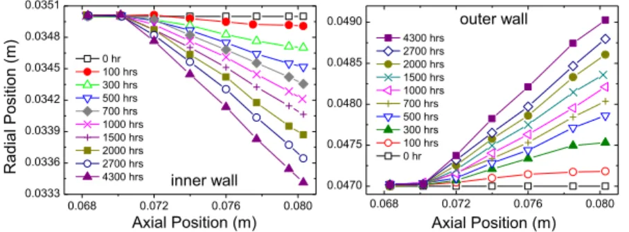
In Fig. 8, the history of erosion of inner and outer walls of the Stanford HT gives a representative vision of how erosion affects the channel wall profiles for a 1 kW-class HT (Sommier et al. 2005). Typically half of the erosion occurs in the first 1000 hours of life. Aa asymmetry in the erosion is also visible Fig. 8, certainly caused by the magnetic topology and non-uniform plasma properties in the radial direction. The origin of the erosion drop is attributed to the angular dependence of sputtering yield which is maximized for an angle of 70 degrees relative to normal incidence (see Appendix 2). Most of ions contribute to erode the surfaces. During the thruster life, the increase of the surface tilt angle has obviously a benefit effect on the reduction of erosion process (Yu and Li 2007). In the literature, during thruster life, a time continuous decrease of the thruster performance has been observed, attributed to a decrease of potential drop inside the channel (Yim et al. 2006) and by a decrease of plasma density (Sommier et al. 2005).
Fig. 8 Simulation of channel wall erosion of the Stanford Hall thruster (from Sommier et al. 2005).
Cheng and Martinez Sanchez (2007) have simulated the operation of the 200 W Busek HT, the BHT-200. Simulated channel wall profiles for 500 hours of operation compare well with experiments, predicting of lifetime of ~ 1300 hours. They have also simulated the BHT-600 and explained higher wall erosion by the presence of doubly charged ions. They highlight the fact that tuning the anomalous coefficients for cross-field transport to successfully capture the erosion profile is not a guarantee that others calculated parameters (discharge current and performance) correspond to experiments (and vice versa). The question of time evolution of anomalous coefficients during the changes of channel geometry is also opened.
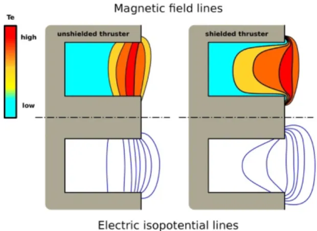
2.8 Magnetic shielded configurations
The strong influence of wall materials on thruster lifetime (through erosion mechanism) and performance (through SEE processes) is an established fact. This is especially true for small size HTs where plasma-wall interactions play a major role. One can imagine pushing the ionization and acceleration regions outside the channel. The so-called wall-less HT is based on this principle. The channel geometry corresponds to the standard one, except that the maximum of magnetic field occurs in the near-field region and the anode position is shifted close to the exhaust. If preliminary results show a decrease of performance, the wall-less configuration takes advantage of keeping a simple magnetic field configuration and the channel length that can be shortened (Mazouffre 2016). In this section, we focus on the proposition of a new magnetic field configuration able to prevent or almost reduce plasma-wall interactions. In the standard magnetic field configuration shown in Sect. 2.5, wall erosion is caused by a non-null radial electric field component that leads to ions generated at the edge of the channel to interact with walls. This is further amplified by a high sheath potential drop induced by a high electron temperature in the acceleration region (see Fig. 8 on the left). An
0.068 0.072 0.076 0.080 0.0333 0.0336 0.0339 0.0342 0.0345 0.0348 0.0351 Radial Po sition (m) Axial Position (m) 0 hr 100 hrs 300 hrs 500 hrs 700 hrs 1000 hrs 1500 hrs 2000 hrs 2700 hrs 4300 hrs inner wall 0.068 0.072 0.076 0.080 0.0470 0.0475 0.0480 0.0485 0.0490 outer wall Axial Position (m) 4300 hrs 2700 hrs 2000 hrs 1500 hrs 1000 hrs 700 hrs 500 hrs 300 hrs 100 hrs 0 hr