Characterization of Fluorohydrogenated Ionic
Liquids for Use in the Ion Electrospray Propulsion
System
by
Caroline Lee Bates
B.S.,
Astronautical Engineering,
United States Air Force Academy
(2016)
Submitted to the Department of Aeronautics and Astronautics
in partial fulfillment of the requirements for the degree of
Master of Science in Aeronautics and Astronautics
at the
MASSACHUSETTS INSTITUTE OF TECHNOLOGY
June 2018
@
Massachusetts Institute of Technology 2018.
A uthor ...
All rights reserved.
Signature redacted
Department of Aeronautics and Astronautics
Certified by ...
May 24, 2018
Signature redacted
I
Paulo C. Lozano
Professor of Aeronautics and Astronautics
Thesis Supervisor
Accepted by ... ... MASS H ISNSMIUTEOFTCNLGY-JUN 28
2018
LIBRARIES
Signature redacted
Hamsa Balakrishnan
Associate Professor of Aeronautics and Astronautics
Chair, Graduate Program Committee
Disclaimer: The views expressed in this thesis are those of the author and do not reflect the official policy or position of the United States Air Force, the United
Characterization of Fluorohydrogenated Ionic Liquids for Use
in the Ion Electrospray Propulsion System
by
Caroline Lee Bates
Submitted to the Department of Aeronautics and Astronautics on May 24, 2018, in partial fulfillment of the
requirements for the degree of
Master of Science in Aeronautics and Astronautics
Abstract
This thesis investigates the use of two fluorohydrogenated ionic liquids as propellants for the ion Electrospray Propulsion System developed at MIT, 1-ethyl-3-methylimid-azolium fluorohydrogenate and trimethylsulfonium fluorohydrogenate. It was found that these ionic liquids undergo a crystallization-like transformation when exposed to vacuum for several hours. Mixtures with a vacuum stable ionic liquid (1-ethyl-3-methylimidazolium trifluoro(trifluoro methyl)borate) were made to study the onset of this transformation and to obtain liquid mixtures from which stable electrospray emission could be obtained. Mixtures containing 10%, 25%, or 50% by mass of one of the fluorohydrogenated ionic liquids are then investigated using time of flight mass spectrometry to determine the beam compositions. All six mixtures operate in the pure ionic regime. Of the six mixtures, the mixture of 25% trimethlysulfo-nium fluorohydrogenate is the best candidate for use as propellant in the ion Elec-trospray Propulsion System, because it produces current 4.8 times higher than pure 1-ethyl-3-methylimidazolium trifluoro(trifluoro methyl)borate, and the beam is com-posed entirely of monomers. Additionally, at voltages used for the ion Electrospray Propulsion System, the 25% trimethlysulfonium fluorohydrogenate mixture has an increase in specific impulse up to 2,000 s over pure 1-ethyl-3-methylimidazolium tri-fluoro(trifluoro methyl)borate. In the appendix, an application of the ion Electrospray Propulsion System is investigated, namely the new WaferSat femtosatellite being de-veloped at MIT Lincoln Laboratory. Motion simulations give preliminary insights into how WaferSats will move in orbit.
Thesis Supervisor: Paulo C. Lozano
Acknowledgments
Above all, I give my thanks and gratitude to my God, Father, Son, and Holy Spirit. I thank You for the opportunity to study at MIT and for sustaining me throughout my time here. I also thank You for my parish family at St. Nicholas GOC and for Fr. Demetri who heard my Confession during my time at MIT. Lord Jesus Christ, Son of God, have mercy on me, a sinner! I also thank the Theotokos and St. Catherine the Greatmartyr of Alexandria for their intercessions on my behalf.
Next, I would like to thank my advisors and mentors at MIT SPL and MIT Lincoln Laboratory, Prof. Paulo Lozano and Dr. Joseph Vornehm. To Prof. Lozano, thank you for the opportunity to work in SPL and for always being willing to help me when I had questions. To Joe Vornehm, thank you for your friendship, for helping me with coding, and for helping me to navigate the transition between undergraduate and graduate student research. I am deeply grateful to my Lincoln Laboratory Group Leader Dr. Kathleen Bihari for welcoming me into her Group and providing the funding necessary for me to attend MIT. I am also indebted to Catherine Miller for the use of her time of flight setup.
Last, but not least, I would like to thank my mom. Thank you for your support, for always answering my phone calls, and for listening to.my complaining about my
"problem liquids."
This work was funded in part by the Air Force Office of Scientific Research
(AFOSR) under award #FA9550-16-1-0273 monitored by Dr. Mitat Birkan. This
material is based upon work supported by the United States Air Force under Air Force Contract No. FA8702-15-D-0001. Any opinions, findings, conclusions or recom-mendations expressed in this material are those of the author and do not necessarily reflect the views of the United States Air Force. MIT Lincoln Laboratory is gratefully acknowledged for their support of this work through the Lincoln Laboratory Military Fellowship program.
Contents
1 Introduction 11
1.1 B ackground . . . . 13
1.2 Ion Evaporation from Ionic Liquids . . . . 16
2 Research 19 2.1 "Crystallization" of FHILs in Vacuum . . . . 19
2.2 Relative Electrical Conductivites of Mixtures . . . . 22
2.3 T im e of Flight . . . . 23
3 Conclusion 35 A Lincoln Laboratory Research: WaferSat 37 A .1 Introduction . . . . 37
A .1.1 Background . . . . 38
A .2 R esearch . . . . 42
A.2.1 WaferSat Motion . . . . 42
A.2.2 Sensitivity to Offset Thrust Vectors . . . . 50
A.2.3 Thruster Control Optimization Using a Genetic Algorithm . . 56
List of Figures
1-1 Thrust density of iEPS compared to Hall thrusters. 1-2 A single porous emitter. . . . . 1-3 Taylor cone. . . . .
2-1 Crystallization of Sill-(HF)1.9F in vacuum. . . . .
2-2 Degrees of crystallization . . . . 2-3 Artistic impression of the degrees of crystallization. . 2-4 Crystallization transition for the FHIL EMI-(HF)2.3F.
Crystallization transition for the TOF setup. . . . . Emitter assembly. . . . . TOF test stand. . . . . TOF results for EMI-(HF)2.3F.
I-V curves for EMI-(HF)2.3F. . .
TOF results for Si1-(HF)1.gF. I-V curves for Slli-(HF)1.gF. . 2-13 Isp bounds for FHIL mixtures. 2-14 Thrust curves for 25% and 50%
FHIL S1il-(HF
3 1 1 -(HF) 1.9F.
Aerospace Corp silicon satellite. . PCBSat. . . . .
SpaceChip . . . .
Two notional designs of SWIFT. . A-5 Sprite flight model...
2-5 2-6 2-7 2-8 2-9 2-10 2-11 2-12 12 15 17 19 21 21 21 22 24 26 26 28 29 30 30 32 33 38 39 40 41 41 A-1 A-2 A-3 A-4 )1.gF. .
A-6 WaferSat with purely radial thruters. . . . . A-7 WaferSat motion example 1.. . . . . A-8 WaferSat motion example 2. . . . .
A-9 WaferSat with thrust vectors directed at 45 . . . .
A-10 WaferSat motion example 3. . . . . A-11 WaferSat with tangentially directed thrust vectors . . . A-12 WaferSat motion example 4. . . . . A-13 Thrust vector offset. . . . . A-14 Trajectory of WaferSat with 0.00010 thrust vector offset A-15 Trajectory of WaferSat with 0.0010 thrust vector offset. A-16 Trajectory of WaferSat with 0.010 thrust vector offset A-17 Trajectory of WaferSat with 0.10 thrust vector offset. A-18 Trajectory of WaferSat with 1 thrust vector offset.
43 46 . . . . 47 . . . . 48 . . . . 49 . . . . 49 . . . . 50 . . . . 51 . . . . 52 . . . . 53 . . . . 54 . . . . 54 . . . . 55
List of Tables
2.1 Relative Conductivities of FHIL Mixtures with EMI-CF3BF3 . . . . . 23
2.2 TOF Results ... ...
A.1 Thrust Vector Offset Summary . . . . A.2 Example GA Outputs . . . . A.3 Error Due to Simulation Time Step . . . . A.4 Simulation Results With Additional GA Runs . . . .
27
55 59 60 60
Chapter 1
Introduction
Miniature satellites are growing in popularity in the space community. These satellites are very small and lightweight compared to traditional satellites. Nanosatellites weigh between 1 and 10 kg, and pico- and fentosats are even smaller. Historically, these tiny satellites have lacked propulsion systems. Chemical propulsion cannot be scaled down to the necessary size, and most types of electric propulsion become too inefficient at the sizes needed by nano- and smaller satellites. One promising propulsion option for miniature satellites is the ion electrospray propulsion system (iEPS) developed by the
MIT Space Propulsion Laboratory (SPL). The iEPS has high specific impulse, and is
scalable to sizes suitable for these satellites.
The purpose of this research is to investigate two fluorohydrogenated ionic liquids (FHILs) for use as propellants in the iEPS. Currently, an iEPS thruster provides thrust on the order of 10 nN per emitter tip. The current iteration of the iEPS thruster array produces 12.5 pN of thrust from 480 emitter tips in 1 cm2
. SPL is seeking to improve the performance of iEPS thrusters by increasing the thrust density. There are two main ways to increase the thrust density of an electrospray thruster. First, the emitter tips in the array can be placed closer together, and therefore have more thrust-producing emitter tips in the same size thruster array. However, there are physical limits to how close emitter tips can be to each other, both in terms of machining ability and how close emitter tips can be before they interact via surface tension and/or electric forces. The second method to increase thrust is to increase the
conductivity of the ionic liquid [1]. As shown later in the text, the emitted current I is linearly dependent on electrical conductivity, K, as given by I = K 327ry2 ( 2
where co is the permittivity of vacuum, c is the dielectric constant of the ionic liquid, -y is the liquid surface tension, and E* is the critical electric field for current emis-sion [2]. Higher emitted currents will result in higher thrust densities. Conventional fuels for iEPS, including 1-ethyl-3-methylimidazolium tetrafluoroborate (EMI-BF 4) and 1-ethyl-3-methylimidazolium bis(trifluoromethylsulfonyl)imide (EMI-Im), have electrical conductivities of K ~ 1 S/rn [1]. In order to increase the electrical con-ductivity at constant temperature another ionic liquid must be used. FHILs display most of the attributes of conventional ionic liquids, like low vapor pressures, but have much higher electrical conductivities. The two FHILs investigated in this thesis are 1-ethyl-3-methylimidazolium fluorohydrogenate (EMI-(HF) 2.3F) and
trimethyl-sulfonium fluorohydrogenate (S1 1 1-(HF)1.9F), with electrical conductivities of K = 10
S/in and K = 13.1 S/m, respectively
I3,
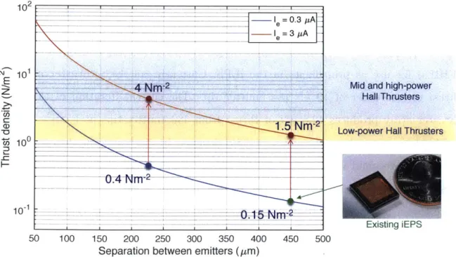
4]. These two FHILs are predicted then to provide current an order of magnitude higher than with the current propellants used in iEPS thrusters. This would put the thrust density of iEPS in line with low-power Hall thrusters [5]. In order to achieve a similar increase in thrust density bymodify-102
1 0.3 1A
-1 =3 A
10-4 2_Mid and high-power
Hall Thrusters
1-5 -- __2'
1.' Nm-2
Low-power Hall Thrusters
Cn 100
10-Existing iEPS
50 100 150 200 250 300 350 400 450 500
Separation between emitters (/im)
Figure 1-1: Thrust density of iEPS compared to Hall thrusters.
12
ing the spacing between emitter tips, they would have to be placed 10 times closer together [6]. Changing the iEPS propellant from EMI-BF4 to either EMI-(HF)2.3F or Smll-(HF)1.gF is expected to produce the ten-fold increase in thrust density without redesigning the iEPS array.
1.1
Background
Electrospray propulsion is a form of electric propulsion that operates by electrostat-ically accelerating charged particles from electrified liquid fuel sources. Unlike other forms of electric propulsion, electrosprays do not need to have a volume for gas phase ionization. This allows electrospray thrusters to be relatively small. In contrast, miniaturizing other forms of electric propulsion, such as Hall thrusters, ion thrusters, and arcjets, increases the heat and energetic ion fluxes to the walls of the thrusters; this decreases the efficiency and life of the thruster
[7].
The first form of electrospray propulsion to be developed was the colloid thruster. Researchers studied these devices between 1960 and 1975 as a possible alternative to ion engines. Colloid thrusters work by accelerating charged droplets, and under special circumstances, ions. They use solvents such as doped glycerol and formamide as propellant. The large molecular mass of the droplets in colloid thrusters appealed to researchers, because in ion engines, a larger molecular mass increases the thrust density of the engine. The colloid thruster research provided useful results, with some being capable of producing a specific impulse, Isp, of approximately 1000 s at accelerating voltages between 10 and 100 kV. However, the high voltages made the colloid thrusters difficult to insulate and package, so they were undesirable for use on spacecraft despite being successful on the ground. Additionally, each individual capillary in the colloid thrusters produced approximately 1 p1N of thrust. Therefore,
in order to produce the amount of thrust for the spacecraft missions anticipated at the time, the arrays of capillaries would have had to be very large
[7].
Although the colloid thruster research of the mid-twentieth century was aban-doned, new research into electrospray propulsion has begun within the past two
decades. This time, the emphasis is on developing propulsion for the new nano- and picosatellites (satellites roughly 10 kg in mass and smaller). In these tiny satellites, the small thrust per emitter that was previously a drawback of the colloid thruster is now an advantage, allowing for fine control of a satellite and higher thruster per-formance. Furthermore, research in the field of electrospray science since the 1970s now allows for electrosprays to operate at more feasible voltages of 1 to 5 kV. Finally, improvements in micro-manufacturing now allow for a large number of emitters to be fabricated on a very small surface. These advances make possible the miniatur-ization of electrosprays. At the MIT Space Propulsion Laboratory, research is being conducted into electrosprays fueled by ionic liquid ion sources, in particular the ion Electrospray Propulsion System (iEPS)[7].
Ionic liquids are also known as room temperature molten salts. They are composed of highly asymmetrical molecular ions that do not form crystalline structures at room temperature. Rather, they are a sea of ions that remain in the liquid state without the presence of a solvent. They are useful in space propulsion for a variety of reasons. Most ionic liquids have practically no vapor pressure, which makes them easy to store in space. Additionally, since ionic liquids naturally consist of free ions, a propulsion system using an ionic liquid as propellant does not need an ionization stage, allowing the propulsion system to be efficient and compact. Most importantly, the electrical conductivity of ionic liquids means that they can be electrically stressed, and thereby produce electrospray emission
[8].
The basic unit of the iEPS electrospray thruster is the single porous emitter. Ionic liquid propellant is held in a reservoir below the emitter. Capillary action pulls the ionic liquid through pores in the emitter and to the tip. Above the emitter tip, an extractor plate applies an electric field at the liquid-vacuum interface, forming a meniscus that collapses into a structure usually called a Taylor Cone [9]. Depending on flow rate, emission could consist of mixtures of ions and droplets or only ions [101.
Romero-Sanz, Bocanegra, and Fernandez de la Mora were the first to discover that ionic liquids could produce emissions composed only of ions without the
pres-/ Emitted Beam Extractor Plate -Electrified Mensicus Emitter Vapp -1-3 kV
Ionic Liquid Reservoir
Figure 1-2: A single porous emitter, adapted from Ref.
[10].
ence of droplets [111. The so-called pure ionic regime (PIR) is the most interesting one as it maximizes efficiency and specific impulse at moderate extraction voltage. The presence of droplets in the mixed ion-droplet regime reduces the efficiency consider-ably. In the pure ionic mode, individual ions field-evaporate from the tip of the cone, are accelerated by the electric field, and pass through a hole in the extractor plate. Within the PIR, ions can either be single ions, called monomers, or larger ions such as dimers and trimers (single ions attached to one or two neutral particles, respectively). Emission of only monomers is the most efficient and therefore the most beneficial for space propulsion. A beam consisting of multiple species of charged particles suffers efficiency losses due to polydispersity. All of the charged particle species in the beam have the same energy, but larger species have slower velocites. As shown in the next section, thrust is linearly dependent on the velocites of the charged particles, so slower velocites result in less thrust [12].
Each individual iEPS emitter provides thrust on the order of 10 nN. In order to produce sufficient thrust for a spacecraft mission, many emitters are arranged together into an array. Currently iEPS arrays contain 480 emitters in a 1 cm2 array, producing 12 pN of thrust
11].
Use of FHILs as propellant should increase the thrust provided by an iEPS array for the same emitter density.1.2
Ion Evaporation from Ionic Liquids
Electrospray propulsion operates by emitting ions from the surface of the ionic liquid propellant. However, ionic liquids have a high energy barrier for ion evaporation. In some cases, the free energy of solvation to extract ions can be as high as 1.5 eV. This energy barrier can be reduced, however, by applying an electric field normal to the surface of the liquid. The equation for the field-evaporated current density is
j= - (T) exp [- (AG - G(E))]. (1.1)
(h kT
Here AG is the free energy of solvation, G(E) is the reduction of the free energy of solvation due to the normal electric field, a is the surface charge density, k is the Bolzmann's constant, T is the temperature, and h is Planck's constant. Current emission is possible when G(E) approaches AG. The reduction of the free energy of solvation, G(E), is described by
re3E
G(E) = . (1.2)
4760
The critical electric field E* for ion evaporation occurs when G(E) ~~ AG,
E ~ 4wreo AG2 (1.3)
The value for E* can be as high as 1.6 V/nm for some ionic liquids. Fortunately, it is not necessary to directly apply such a high electric field to the ionic liquid to operate an electrospray thruster
18].
If a large enough electric field is applied normal to the ionic liquid, the liquid deforms and collapses into a Taylor cone, illustrated in Figure 1-3. This Taylor cone is formed by the balance between the pressure caused by the electric field and the surface tension of the liquid, as shown by the equation
S 2 YcotO (1.4)
where E0 is the permittivity of vacuum, E" is the electric field acting normally on the
liquid, 7 is the surface tension of the liquid, 0 is the angle of the Taylor cone, and r is the distance from the tip of the cone to a point on its surface. Equation 1.4 can be rewritten to find the normal electric field
En 2cot 0 (1.5)
S 60T
171
As r decreases, E, increases; let r = r* be the distance that makes E = E*, thecritical field needed for ion evaporation 1].
r n
Figure 1-3: Taylor cone, from Ref. [7].
While theoretically the Taylor cone is a perfectly shaped cone, in reality it does not end in a sharp point. Rather, the meniscus that forms has a blunt structure with a curvature at its apex of 2/r*. For ionic liquids, the conductivity of the liquid is low enough that it forces the charge density to be far from fully relaxed (o- < EoE*). The electric field inside the Taylor cone then is approximately Ej" ~ E*/6. For the case of equilibrium, the mechanical balance at the curved interface of the Taylor Cone is
EE*2 - jE0EEla ~ 2y/r*, which gives 4-,e
Assuming a half-sphere current emission, the total current I is I = 2jr*2 where
j
is the current density emitted from the surface of the meniscus. Neglecting convection, charge transport is due only to the liquid conductivity such that j = KEm ~ KE*/e.Thus, the emitted current becomes,
I (327K> 2
) 6 (1.7)
6eE*3
6 _ 1)2This linear relationship between emitted current and conductivity provides the mo-tivation for this work. EMI-(HF)2.3F and Sill-(HF)1.F have conductivities an order of magnitude higher than that of EMI-BF4. Therefore, an electrospray thruster
us-ing either of these FHILs as fuel should have an emitted current up to an order of magnitude higher than an electrospray thruster using EMI-BF4. Assuming the mean
specific charge for emitted species is q/m, the ideal thrust produced by an electrospray emitter will be given by,
F=mv= 2-V, (1.8)
qlm n
where I is the current, and V is the applied voltage
[13].
Thrust is proportional to current, which is proportional to conductivity. So, a thruster using EMI-(HF)2.3F or Smll-(HF)1.9F will provide thrust up to an order of magnitude greater than a thrusterusing EMI-BF4 at similar voltages and charge-to-mass ratios, simply because of the
Chapter 2
Research
2.1
"Crystallization" of FHILs in Vacuum
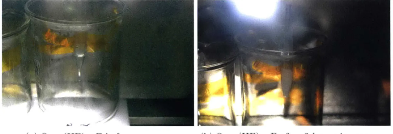
Both EMI-(HF)2.3F and Smll-(HF)1.F in their pure forms adopt a "crystal"-like struc-ture when exposed to vacuum. This is problematic for space propulsion as the pro-pellant becomes unusable in its solid form. The high electrical conductivity of these ionic liquids, however, is anticipated to improve the thrust performance of iEPS.
(a) Slli-(HF)1.9F before vacuum. (b) S1il-(HF)1.9F after 3 hours in vacuum. Figure 2-1: Crystallization of Smll-(HF) 1.9F in vacuum (in tip of dropper). Note the
clear color of the liquid phase before vacuum, and the cloudy appearance due to crystal-like structure formation after 3 hours in vacuum.
Therefore, it was hypothesized that mixtures of these FHILs with ionic liquids that are known to be stable in vacuum might produce combinations that will remain as liquid while improving the conductivity. Initial experiments to determine the crystallization
boundaries of the FHILs used EMI-Im. However, EMI-Im was replaced by 1-ethyl-3-methylimidazolium trifluoro(trifluoro methyl) borate (EMI-CF3BF3), because of the
higher conductivity of EMI-CF3BF3. This liquid has a conductivity of 1.46 Si/m at
25' C [14], similar to that of EMI-BF4. EMI-CF3BF3 has a lower electrical
conductiv-ity than the two FHILs, but it has the advantage of remaining in a liquid state when exposed to vacuum. Since EMI-(HF)2.3F and Sil-(HF)1.gF have higher conductivities than EMI-CF3BF3, the mixtures should have as high a concentration of the FHILs
as possible. Therefore, the first experiment to be done was to determine the highest possible concentration of each FHIL that can be mixed with EMI-CF3BF3 without
the mixtures crystallizing.
Mass fractions of FHIL were chosen around the suspected crystallization bound-ary. Each mixture was placed in an individually marked Teflon dish. Each mixture had a mass of approximately 0.20 g. First, the desired mass of one of the FHILs, ei-ther EMI-(HF)2.3F or Sil-(HF)1.gF, was dropped in the Teflon dish using a syringe. Next, EMI-CF3BF3 was added to the Teflon dish to bring the total mixture mass to
approximately 0.20 g. The Teflon dishes were then placed in a vacuum chamber for approximately two days, where the pressure was below 1 x 10⁻⁵ Torr. Throughout the two days, the mixtures were observed through a window in the vacuum chamber and any crystallization was recorded. Figure 2-2 shows photographs of actual FHIL mixtures in the possible degrees of crystallization, while Figure 2-3 shows an artistic impression of the same for the sake of clarity. There are five degrees of crystallization separated into three regions. The first degree is no crystallization, and occurs when the fraction of FHIL in the mixture is below the crystallization transition region. The next three degrees of crystallization occur in the transition region. The second degree of crystallization happens when the mixture contains a few crystals. The third degree of crystallization happens when the mixture has a slushy consistency. Many crystals form in the mixture, but the mixture is still mostly liquid. The fourth degree of crystallization is the last one in the transition region and occurs when the mixture is roughly half crystals and half liquid. The final region is complete crystallization of the mixture. Mixtures in this region are mostly crystals, and at the extreme end of
100% FHIL they are completely crystallized solids.
(a) Degree 1. (b) Degree 2. (c) Degree 3. (d) Degree 4. (e) Degree 5.
Figure 2-2: Degrees of crystallization
20
2
1
3
4
5
Figure 2-3: Artistic impression of the degrees of crystallization.
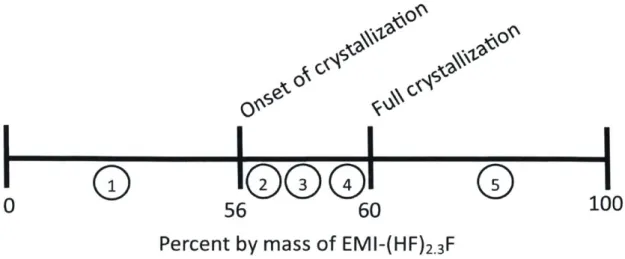
Mixtures of EMI-(HF)2.3F with EMI-CF3BF3 remain liquid below concentrations
of 56-60% EMI-(HF)2.3F by mass. A line plot of the crystallization transition for
EMI-(HF)2.3F is shown below in Figure 2-4. The numbers 1-5 correspond to the
degrees of crystallization shown in Figures 2-2 and 2-3.
KN
0 \
0 \
IKN0
0 1
0
I
I
IQ'00
56
60
0)
Percent by mass of EMI-(HF)
2.
3F
Figure 2-4: Crystallization transition for the FHIL EMI-(HF)2.3F.
I
I
0
I
I
100
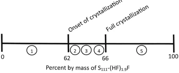
The same crystallization phenomenon occurs in S il-(HF)1.gF. The crystallization transition region occurs at 62-66% S111-(HF)1.9F. Figure 2-5 shows the line plot for the
crystallization of S1il-(HF)1.F. Sill-(HF)1.gF crystallizes at a higher concentration
I~~~
0100
0
62
66
100
Percent by mass of Smll-(HF)
1.
9F
Figure 2-5: Crystallization transition for the FHIL S1il-(HF)1.9F.
than EMI-(HF)2.3F. This should allow for mixtures with higher concentrations of the
FHIL, and therefore increased emitted current.
2.2
Relative Electrical Conductivites of Mixtures
Once the crystallization boundaries of the two FHILs were determined, three concen-trations of each FHIL were chosen for future experiments. For both EMI-(HF) 2.3F
and Sill-(HF) 1.9F, concentrations of 10%, 25%, and 50% were investigated. All of
these concentrations are below 56% FHIL, which is the boundary where EMI-(HF) 2.3F
begins to crystallize. Although Si1-(HF) 1.gF has a higher crystallization boundary, the same concentrations of both FHILs were chosen for comparison purposes between the FHILs.
For each of these concentrations, the relative conductivity of the mixtures at room temperature were determined using the conductivity of EMI-CF3BF3 as the baseline.
The relative conductivity of each mixture was determined by measuring the resistance through the mixture. A thin capillary was filled with a mixture. Platinum wire was
inserted into each end of the capillary, and an ohmmeter was used to determine the resistance through the mixture. The platinum wire was inserted approximately the same distance inside the capillary for all the mixtures. Resistance and conductivity are inversely related in the equation K = , so the relative conductivity of each
mixture was determined by dividing the resistance of the mixture by the resistance of the pure EMI-CF3BF3.
The results of the relative conductivity test are summarized in Table 2.1. These Table 2.1: Relative Conductivities of FHIL Mixtures with EMI-CF3BF3
FHIL Concentration Relative Conductivity
0% FHIL (100% EMI-CF3BF3) 1 10% EMI-(HF)2.3F 1.8 25% EMI-(HF)2.3F 3.7 50% EMI-(HF)2.3F 5.5 10% Sill-(HF)1.gF 1.8 25% Sill-(HF)1.gF 2.3 50% Sill-(HF)1.gF 3.4
results show a general pattern of increased conductivity as the mass fraction of FHIL increases. Although Sill-(HF)1.9F has a higher conductivity than EMI-(HF)2.3F,
the EMI-(HF)2.3F mixtures have a higher relative conductivity for the same mass
fraction of FHIL. This is an interesting, unexplained result. Future work should probe the possible reasons for this apparent contradiction of expectations. It is also possible that the result is due to measurement error, which was not estimated in these measurements, or to procedural error. Additional conductivity measurements are underway, and results will be reported in the future.
2.3
Time of Flight
The final experiment was the characterization of how each mixture behaved when fired from a single carbon xerogel emitter. Current-voltage (I-V) curves and time of flight (TOF) tests were used to characterize the performance of each FHIL mixture.
TOF spectrometry is used to determine the composition of the emitted ion beam. The setup, a diagram of which is shown in Figure 2-6, consists of a deflector gate and a channeltron which collects the emitted beam. The deflector gate is turned on and off. When the gate is on, charged particles are deflected away from the channeltron. When the gate is off, charged particles are allowed to flow to the channeltron, where they are collected. The lighter ions arrive at the channeltron first, followed by the heavier ions and droplets. From the current received by the channeltron over time, it can be determined which charged species are in the beam and what percentage of the beam is composed of monomers, heavier ions such as dimers and trimers, or other species, like charged droplets [15].
Emitter Deflector Gate
Extractor Plate
I
~
-95 V
Gate ON...] Channeltron
- - - --------------
-Gate OFF out
Vapp +950 V
Figure 2-6: TOF setup, adapted from Ref. 115] and 110].
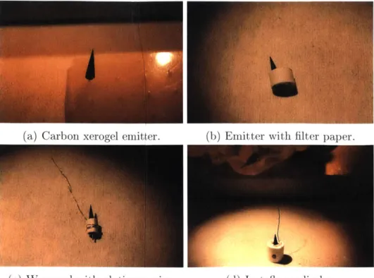
Preparation of the TOF setup requires multiple steps. First, the emitter must be fabricated. The emitters used in this experiment were made of resorcinol formalde-hyde carbon xerogel. This material was made by mixing a solution of resorcinol, formaldehyde, acetone, and water. This solution was then poured into cylindrical spaces in a mold. Into each cylindrical space, a 1 mm diameter stainless steel rod was inserted. This rod was used later in the process to hold the carbon xerogel cylinder while sharpening the emitter tip. The mold was placed into a closed container to set for 24 hours. After 24 hours, the container was placed in an oven to cure for four
days. Over the course of the four days, the temperature of the oven was increased from 40'C to 80 C. Then the container was taken out of the oven and its lid removed, permitting the resorcinol formaldehyde emitters to dry, and the container and the mold then sat in the fume hood for 24 hours. After 24 hours, the open container holding the mold was then placed back into the 80'C oven for a final 48 hours [101.
After the final 48 hours, the container was removed from the oven and the mold was allowed to cool. Once the mold cooled, the solid resorcinol formaldehyde emitters were removed from the mold. The emitters were then sharpened into a cone with a half-angle of ~ 100 using a Dremel tool and sandpaper. The stainless steel rod in the emitter was held by the Dremel, and the Dremel spun the emitter, sharpening the other end on the sandpaper. After the carbon xerogel emitters were sharpened, they were pyrolized in a 900'C tube furnace for four hours while 400 sccm argon gas flowed over them. Once an emitter tip was pyrolized it was ready for use. The emitters used in this experiment were created by Dr Perez-Martinez. Further details on how the emitters were sharpened can be found in Ref. [10].
After the tip was pyrolized, most of the stainless steel rod was cut off. The emitter was then wrapped with HF-compatible filter paper and a platinum wire was wrapped around the filter paper to secure it. The platinum wire was also later used to connect the emitter with the high voltage source. The emitter, filter paper, and platinum wire were then placed in a porous Teflon cylinder. The Teflon cylinder was then set into the TOF test stand. Next, the end of the platinum wire was wrapped around a set screw. A nut secured the platinum wire, followed by another wire which connected to the high voltage source and was secured with another nut on the set screw. The assembly process is shown in Figure 2-7.
Finally, the extractor plate was placed on the test stand above the emitter and the emitter tip was centered on the hole in the extractor plate. The final setup is shown in Figure 2-8. The test stand was then attached to the flange of the vacuum chamber, and the vacuum chamber was sealed and pumped down to below 1 x 10⁻⁵
Torr.
(a) Carbon xerogel emitter. (b) Emitter with filter paper.
(c) Wrapped with platinum wire. (d) In teflon cylinder.
Figure 2-7: Emitter assembly.
(a) Angled view of TOF test stand. (b) Side veiw of TOF test stand.
Figure 2-8: TOF test stand.
gate electrodes was 1900 V. Further details of the TOF test setup can be found in Ref [15]. TOF experiments were done for mixtures of both EMI-(HF)2.3F and Sur
(HF)1.9F at concentrations of 10%, 25%, and 50%. For each mixture, TOF data was
recorded on the oscilloscope for a 200-300 V range of applied voltages in the positive
mode with intervals of 50 V. Five to ten sets of TOF data were taken for each FHIL mixture. Due to the difficulty of fabricating emitters with sufficiently sharp tips, two were used to conduct all of the TOF experiments. In between testing different
mixtures, the emitter was cleaned in sonic baths of isopropanol and acetone and the tip hand-sharpened on a small piece of 2500-grit sandpaper. However, the reuse and hand-sharpening resulted in emitter tips that became less sharp over time.
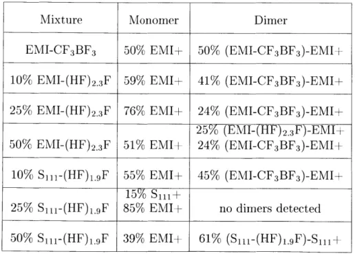
Ideally, electrospray thrusters should operate in the pure ionic regime (PIR), meaning the charged particle beam is completely composed of ions without the pres-ence of droplets. Within the PIR a beam composed solely of monomers is beneficial. A beam composed solely of monomers maximizes Isp, because it contains only the fastest, lightest-weight charged species. In cases where the beam contains only one species of ion, this beam will also be more efficient, because there will be no poly-dispersity and all the ions will be accelerated to the same velocity. All six mixtures operated in the PIR, with beams composed only of monomers and dimers. Table 2.2 summarizes the results of the TOF testing. Pure EMI-CF3BF3 was used as a baseline
for comparison against the FHIL mixtures. Pure EMI-CF3BF3 is roughly 50% EMI+
Table 2.2: TOF Results
ions (monomers), and 50% (EMI-CF3BF3)-EMI+ dimers. As the amount of FHIL in
the mixture was increased, the percent of monomers increased and dimers were
sup-Mixture Monomer Dimer
EMI-CF3BF3 50% EMI+ 50% (EMI-CF3BF3)-EMI+
10% EMI-(HF)2.3F 59% EMI+ 41% (EMI-CF3BF3)-EMI+
25% EMI-(HF)2.3F 76% EMI+ 24% (EMI-CF3BF3)-EMI+
25% (EMI-(HF)2.3F)-EMI+ 50% EMI-(HF) 2.3F 51% EMI+ 24% (EMI-CF3BF3)-EMI+
10% S1il-(HF)1.gF 55% EMI+ 45% (EMI-CF3BF3)-EMI+
15% Sil+
25% Sill-(HF)1.gF 85% EMI+ no dimers detected
pressed. However, past a certain point, adding FHIL did not increase the percentage of monomers in the beam. Instead, for both EMI-(HF)2.3F and Smt-(HF)1.gF the
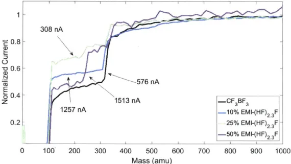
mix-tures of 50% FHIL had a lower percentage of monomers than the 25% FHIL mixmix-tures. Figure 2-9 shows the TOF results for the EMI-(HF)2.3F mixtures. The presence of
308 nA -0.8--o 0.6--a 576 nA 00.4 z 1513 nA -CF 3BF3 1257 nA -10% EMI-(HF) 23 F 0.2-1 25% EMI-(HF) F--50% EMI-(HF) F 0 100 200 300 400 500 600 700 800 900 1000 Mass (amu)
Figure 2-9: TOF results for EMI-(HF)2.3F.
EMI-(HF)2.3F suppressed some of the emission of dimers, but not all. The 50%
EMI-(HF)2.3F mixture contained both (EMI-CF3BF3)-EMI+ and (EMI-(HF)2.3F)-EMI+
dimers, while in the other mixtures only (EMI-CF3BF3)-EMI+ was present. The
optimum mixture for EMI-(HF)2.3F in which all dimers and larger charged particles
are suppressed probably occurs between 25% and 50% EMI-(HF) 2.3F. Further testing
should be conducted to find this optimum.
I-V curves were also performed for all the mixtures. Figure 2-10 compares the results for the EMI-(HF)2.3F mixtures against pure EMI-CF3BF3. The 10%
EMI-(HF)2.3F performed the best. However, this is most likely due to the order of testing.
The 10% EMI-(HF)2.3F mixture was the first mixture to be tested. The emitter
tip was therefore very sharp and unused. This explains why the 10% EMI-(HF) 2.3F
produced more current at lower voltages. Further experiments should be conducted with separate, identical emitters for each FHIL mixture in order to obtain a more
accurate comparison between the mixtures. 2000 1500- 1000S:500 -- 0--500 A-EMI-CF 3BF 3_ -10% EMI-(HF) F -1000 25% EMI-(HF)2 3 F -50% EMI-(HF)2 3 F -1500 ' -3000 -2000 -1000 0 1000 2000 3000 Voltage (V)
Figure 2-10: I-V curves for EMI-(HF) 2.3F.
For Sil-(HF)1.gF, the optimum mixture for Isp is 25% Sill-(HF)1.gF. In this
mix-ture, the beam is entirely monomers. While all the Sil-(HF)1.gF beams contained
EMI+, the 25% Slli-(HF)1.9F beam also contained Sil+ monomers, which comprised
15% of the beam. The 50% Sill-(HF) 1.9F beam contained the lowest percentage of
EMI+ monomers, and also contained (Sill-(HF)1.9F)-S1 + dimers. Figure 2-11 shows
the TOF results for the Si1 -(HF) 1.9F mixtures.
Not only did the 25% Sill-(HF) 1.9F mixture beam produce only monomers, but
this mixture also produced the most current. Similar to the EMI-(HF) 2.3F mixtures, the significantly higher current produced by the 25% S1il-(HF)1.gF mixture might be caused in part by a sharper tip. However, this mixture was the last mixture to be
tested, after the emitter had been hand-sharpened many times. The 10% and 50%
S1il-(HF)1.9F mixtures performed better than the EMI-CF3BF3 baseline, but did not
show significantly increased current like the 25% Sill-(HF)1.gF. The I-V curves for
the Si1 -(HF)1.9F mixtures are shown in Figure 2-12.
3024 nA ~576 nA 1476 nA -F3B -CF 3BF3 756 nA -10% S111-(HF)19F 25% S -(HF) F --50% Sl l-(HF), 9F 0 100 200 300 Figure 2-11: 400 500 600 700 800 900 1000 Mass (amu)
TOF results for Slli-(HF)1.gF.
-CF3BF3 -10% Slll-(HF) 9F -25% S11 -(HF) 9F -50% S -(HF) F -1000 Figure 2-12: I-V 0 Voltage (V) curves for 1000, S1il-(HF)1.9F.
to test multiple mixtures, the data shows a clear improvement by adding FHILs to EMI-CF3BF3. The EMI-(HF)2 3F mixtures all showed an increase in the percentage
of monomers in the beam over the EMI-CF3BF3 baseline. All three S11i-(HF)I.9F mixtures showed an increase in current over EMI-CF3BF3. All six FHIL mixtures
operated in the PIR, producing only monomers and dimers. The TOF and I-V data
1 E 0 z 0.8 0.6 0.4 0.2 8000 - 6000- 4000-2000 C C a) L. 0 0 -2000--4000,,, -6000' -3000 -2000 2000 3000 i i i i
presented above suggests that there is an optimum mixture ratio for the FHILs that optimizes current and the presence of monomers in the beam. However, this should be investigated in future work in which a different emitter is used for each FHIL mixture. Different mass fractions of FHILs produced varying degrees of clustering in the beam. In the case of 25% S1il-(HF)1.9F, the mixture produced both high current
and a beam composed solely of monomers.
The TOF data was then used to determine the average charge-to-mass ratios for the 25% Sill-(HF)I.9F and 50% Sill-(HF) 1.gF mixtures and calculate the performance characteristics Isp and thrust for each. These mixtures have the highest percentage of monomers or dimers, respectively, and therefore represent the upper and lower bounds of the performance of the FHIL mixtures. Both I, and thrust in electrospray thrusters are dependent on the voltage to the extractor plate. Isp is calculated using the equation I th qutonIp 9 1 7h1 2V, where - is the average charge-to-mass of the charged particles in the beam and V is the voltage. The force of thrust is calculated using the equation F = I J . In the TOF experiments, voltages up to 3,000 V were applied to the extractor plate. However, for iEPS, operational voltages range between 700 V and 2000 V.
In Figure 2-13 voltage versus Isp is plotted for the baseline EMI-CF3BF3, 2 5%
S1il-(HF)1.9F, and 50% Si-(HF)1.gF for the range of voltages used in iEPS. While the 50% S1il-(HF)1.gF mixture had a lower percentage of monomers than the EMI-CF3BF3 baseline did, the presence of the lighter (S11 -(HF)1.9F)-Si1 + dimer in the
beam lowered the average mass of the charged particles in the beam. The lower av-erage masses in the 25% Sj1i-(HF)1.9F and 50% Sill-(HF)1.gF mixtures resulted in higher Isp than for EMI-CF3BF3 for the same voltages. At 2,000 V, the 25%
Sill-(HF)1.9F mixture had an Is, 2,000 s higher than EMI-CF3BF3 did.
The other important performance characteristic is thrust. The calculated thrust curves for 25% and 50% Sjji-(HF)1.9F are shown in Figure 2-14. For these
calcu-lations, the same voltage range was used, and current was varied between 0.5 pA and 2pA. Because thrust is inversely proportional to the square of the charge-to-mass
6500 6000 5500 5000 's 4500 - 4000 3500 3000 2500 2000 -CF 3BF 3 -25% S111 -.50%S -(HF) F 600 800 1000 1200 1400 1600 1800 Voltage (V)
Figure 2-13: Isp bounds for FHIL mixtures.
2000 2200
ratio and the 50% Smil-(HF) 1.gF mixture had a higher average mass, this mixture pro-duced higher thrust for the same voltage and current. If the thrust for EMI-CF3BF3
were plotted, it would show even higher thrust for the same current, because the EMI-CF3BF3 beam had an even higher average mass. However, in the above TOF
experiments, the 25% Smll-(HF)1.9F mixture produced significantly higher current
than EMI-CF3BF3 and the other Sm1-(HF)1.9F mixtures for the same voltages, up
to an almost five-fold increase over EMI-CF3BF3. Therefore, when the same voltage
is applied, the current produced by the 25% Smll-(HF)1.gF mixture should increase, producing higher thrust than EMI-CF3BF3.
600 800 1000 1200 1400 1600 1800 2000 2200 Voltage (V)
(a) Thrust curves for 25% S1 1-(HF)I F.
-0.5 gA - -I uA 1.5 MA -- 2 pA 600 800 1000 1200 1400 1600 1800 2000 2200 Voltage (V)
(b) Thrust curves for 50% S1 1 1-(HF)1.9F.
Figure 2-14: Thrust curves for 25% and 50% S1il-(HF)1.gF. 140 120 100 F -0.5 p -1 IA -2.5 p -2piA 1-1 z 80- 60-40 20 0 180 160 140 ,t H 120 100 80 60 40 20 I I I A... ... A ...
Chapter 3
Conclusion
FHILs are a promising method for increasing the thrust density of iEPS. However, because EMI-(HF)2.3F and Sil1-(HF) 1.gF crystallize in vacuum, it was necessary to investigate mixtures of these FHILs with EMI-CF3BF3. The first experiment in this
thesis determined the crystallization transition region of the two FHILs. For EMI-(HF)2.3F, this transition occurred from 56% to 60% concentration by mass, and for
Si1-(HF)19.F the transition occurred between 62% and 66%. Once the crystallization
transition regions of the two FHILs were found, varying concentrations of the FHILs below their crystallization boundaries were investigated using TOF to determine their beam compositions. For both FHILs, concentrations of 10%, 25%, and 50% were investigated. The TOF results showed that all six FHIL mixtures operated in the PIR. The 25% Sill-(HF)1.gF mixture was unique in that it produced only monomers. Within the range of voltages used for iEPS, this mixture had an improvement in ISP up to 2,000 s over EMI-CF3BF3. For the same current and voltage, the 25%
Si1-(HF)1.gF mixture had lower average mass than EMI-CF3BF3. However, since
the 25% S1il-(HF)1.gF produced much higher current density, it should ultimately produce more thrust than EMI-CF3BF3 for a given applied voltage.
This research demonstrates that FHILs are a good additive to EMI-CF3BF3 for
use as iEPS propellant, in particular the 25% Sill-(HF)1.gF mixture. It produced a
significantly higher current than the baseline EMI-CF3BF3 did and emitted a beam
being well below the crystallization transition region for Smll-(HF)1.9F.
This work also raises important questions to be answered by future research. While I believe the trends in my TOF and I-V measurments to be accurate, re-peating them with a new carbon xerogel emitter for each mixture will increase the precision of the measurement and increase confidence in the result. Additional re-search should also be conducted to determine if EMI-(HF)2.3F has an optimum mass
fraction that maximizes the emission of monomers, greatly increases the produced current, or both. Future TOF work could also include investigating Smll-(HF)1.9F
mixtures around 25% for a more precise value of the optimum mass fraction. The reasons for EMI-(HF)2.3F mixtures demonstrating higher relative conductivity than Smll-(HF)1.9F mixtures should be investigated, as they may shed new light on the
use of FHIL mixtures and hint at optimizations to be made. Such investigations could begin with repeated conductivity measurements to establish statistical error bounds on the results. Finally, research should also be conducted into what causes the crystallization of the pure FHILs and mixtures containing high percentages of FHIL.
Appendix A
Lincoln Laboratory Research:
WaferSat
A.1
Introduction
WaferSat is a new type of miniature satellite being developed at MIT Lincoln Lab-oratory, constructed on silicon wafers. The WaferSat bus will be cheap to produce in bulk, at an expected price point of $15,000 per satellite, allowing end users to put tens, hundreds, or even thousands of them into space for less than the cost of a larger satellite, which can easily exceed $1 billion. Possible missions for WaferSat constel-lations include investigation of the Earth's ionosphere and synthetic large aperture imagery. Like most satellites, but unlike many other minature satellites, WaferSats will have an on-board propulsion system. This propulsion system is modeled after the iEPS from MIT SPL.
Since WaferSats have an unusal combination of size, mass, and shape, a study of their motion is necessary. This study, conducted in MATLAB, was a general first pass at understanding how a WaferSat will move in space. It assumed a 2-D frictionless plane, point thrusters, and no external forces (such as gravity or drag), in order to provide a basic understanding of how an individual WaferSat will move within its orbit. The process of developing the simulator began with describing the basic translational and rotational motion of a WaferSat when subjected to the force
from a single thruster. Next, combinations of thruster firings were added to the simulation to allow for more complex maneuvering. After that, thruster position offset was investigated to determine the WaferSat's sensitivity to misalignment of thrusters. Finally, a genetic algorithm was investigated for its future use in creating firing command sequences to move the WaferSat to a desired location.
A.1.1
Background
The space community has been interested in the idea of a "satellite-on-a-chip" since at least 1994, when the idea was first proposed [16, 17]. In 1999, Janson of Aerospace Corp. proposed a batch-produced, "system-on-a chip" satellite made of silicon[18]. The proposed satellite, shown in Figure A-1, was a thick cylindrical "stacked multi-wafer system", the dimensions of which were 10 - 30 cm.
4tt
Figure A-1: Aerospace Corp silicon satellite, from Ref. [181.
This proposed satellite included a propulsion system to facilitate the control of clusters and constellations of the satellites. One proposed propulsion system concept was digital micropropulsion, an array of shot thrusters. Each of these single-shot thrusters would be a microcavity containing propellant and an ignitor, and would be individually sealed and controllable. Thousands of microthrusters would allow the spacecraft to perform hnndreds of maneuvers in orbit. A major drawback of
this design is the one-time use of each microthruster. If the spacecraft fired all of the microthrusters in one location, it would be unable to perform future maneuvers. Janson also briefly proposed a microfabricated resistojet (a type of electric propulsion that operates by heating propellant and then expanding it through a traditional nozzle) as the propulsion system instead
118].
However, as the size of a resistojet is decreased, so too is its efficiency. Aerospace Corp never fabricated any of this silicon wafer-based satellite.In the same year that Janson proposed his silicon spacecraft, the Surrey Space Centre in the UK set a goal to build a "satellite-on-a-chip" [161. This would be a true stand-alone on-a-chip, as opposed to a stack of silicon wafers. The system-on-a-chip design was attractive, because of its potential mass producibility and low cost per unit. These same benefits are also drivers behind MIT Lincoln Laboratory's current WaferSat project. The Surrey Space Centre developed a prototype, named "PCBSat", which was a 70 g satellite-on-a-PCB, shown in Figure A-2. Although the prototype PCBSat was fabricated, none were ever launched.
-4MHz scontroller l&V Telemetry 3.3V Regulator, PPT & BCR
CMOS Imager RT Clock GPS Receiver 2A G~zand antenna Radio Module -ioit (-2 km -on battery rang.) 9 x 9.5 cm
Figure A-2: PCBSat, from Ref. [19].
Surrey Space Centre's conceptual design, SpaceChip, shown in Figure A-3, was to be the first monolithic satellite-on-a-chip. It was proposed as a solution for distributed missions, such as distributed aperture radar, that require a large number of nodes. A generic mission design would include a large number of SpaceChips which would be deployed from a mothership in low Earth orbit (LEO). The mothership would
Digital Radio Power Control Central Processing unit Antennas 18X20111m1 Processor Solar Cells C O CMOs Imager
Figure A-3: SpaceChip, from Ref. [161.
then relay information between the cluster of SpaceChips and the ground station. The SpaceChip bus would have many of the same subsystems as larger spacecraft, including structural, electrical power, data handling, and communication subsystems. Notably, SpaceChip would not have a propulsion subsystem. This lack of a propulsion subsystem combined with atmospheric drag would result in a short operating life for the SpaceChip cluster. The design of SpaceChip included a maximum circuit area of 360 mm2 and a maximum mass of less than 10 g [16]. No SpaceChips were ever fabricated or launched.
The next proposal for tiny, inexpensive satellites was the Silicon Wafer Integrated Femtosatellite (SWIFT) developed by Chung and Hadaegh at NASA's Jet Propul-sion Laboratory (JPL). The goal of this project was to be able to create a distributed aperture array composed of a swarm of "fully capable femtosats" [201. Chung and Hadaegh defined "femtosat" as the 100 g class of spacecraft. Each satellite would be manufactured using "3-D silicon wafer fabrication and integration techniques" and would be actively controlled in all six degrees of freedom [20]. JPL developed sev-eral key subsystem requirements for the SWIFT spacecraft. These included an Is, of greater than 100 s, and a AV of 24 m/s for a three-month mission [21]. SWIFT would therefore need a propulsion subsystem. Two notional designs, shown in Figure A-4, include either a digital microthruster system, similar to the propulsion subsystem proposed by Janson for his satellite, or a miniaturized warm gas hydrazine system. Hadaegh, Chung, and Manohara also proposed electrospray thrusters for the propul-sion subsystem, which would use either indium or ionic liquid propellant [21]. The
(a) Micropropulsioni. (b) Warm hydrazine.
Figure A-4: Two notional designs of SWIFT, from Ref. [21J.
total mass of the propulsion subsystem was required to be less 40 g. However,they had difficulty meeting this mass requirement, stating that the "development of a fully capable 100-g-class feitosat hinges on ... the successful miniaturization of the propul-sion system" [211. The SWIFT propulpropul-sion system would require two thrust levels: a high thrust of approximately 100 pN to position the spacecraft in orbit and a low thrust of approximately 10 IN for station-keeping. On the larger, satellite-wide scale, Hadaegh, Chung, and Manohara decided to design SWIFT using primarily chip-level integration, rather than the wafer-scale integration they originally proposed. Wafer scale integration was proposed instead for occasional use in manufacturing the fem-tosats. Initially wafer scale integration was proposed because it would result in a low-power spacecraft, but it was less modular and more expensive than chip-level integration. No SWIFT spacecraft were ever produced
[21].
The final "satellite-on-a-chip" precursor to WaferSat was the Sprite satellite devel-oped at Cornell University [22J. Sprites were 3.5 cm by 3.5 cm satellites weighing 5 g. A flight model is shown in Figure A-5. They did not have a propulsion subsystem.
Gyroscope .- Solar Cells
Microcontroller
Magnetomneter
C- Antenna
Radio /
Chemical propulsion and ion engines cannot be scaled down to the size needed for Sprites, but Atchison and Peck proposed the possibility of adding digital propulsion to future iterations of the Sprite. While Sprites lacked a propulsion subsystem, they did have other traditional subsystems including communication and power [231. The basic mission for Sprites involved a mothership called KickSat from which 128 Sprites would deploy. Sprites were expected to spend only a few days in orbit before reenter-ing Earth's atmosphere
1221.
KickSat and 128 Sprites were launched in April 2014; however, the Sprites were not able to deploy from the KickSat mothership before itdeorbited 124].
WaferSat shares many similariteis with its predecessors. It is designed to be a low-cost, mass-producible satellite bus, which can be used for many types of missions including distributed aperture radar, space weather monitoring, and communication relays. Like SWIFT and the system-on-a-chip design proposed by Janson, WaferSat will have a propulsion system. However, this propulsion system will be an electrospray propulsion system based on the iEPS developed at MIT SPL. Unlike in the previous spacecraft designs, the WaferSat structure will be a bonded stack of a few 200 mm diameter silicon wafers
125].
It will be smaller than Janson's satellite and SWIFT,but large enough for a propulsion sytem, and have a unique disk shape.
A.2
Research
A.2.1
WaferSat Motion
WaferSats have the potential to be used for a variety of missions. However, they have a unique shape for satellites, and the effect of the disk shape on orbital motion must be investigated. The simplest orbit for a satellite is a circular orbit with a semi-major axis a = Re + alt, where Re is the mean radius of the earth, 6378 km, and alt is the satellite's altitude. In this study, the motion of a WaferSat was constrained to a few kilometers. The space the WaferSat was operating in was much smaller than the semi-major axis of its orbit. Therefore, for the purpose of this study, the WaferSat
was assumed to move in a 2-D x-y plane. To further simplify the problem, the plane
was frictionless and external forces such as gravity and drag were ignored.
WaferSat has a radius of 0.1 m, and for the purpose of this study had a mass of 50 g. This mass is on the low end of the projected range of masses for the WaferSat bus. WaferSat will have two types of thrusters: in-plane and out-of-plane. In-plane thrusters will be used for orbit changing and station-keeping, and in this study the thrusters controlled the WaferSat's motion in the x - y plane. Out-of-plane thrusters will provide attitidue control by providing rotation about the WaferSat's x- and y-axes. This study focused on the in-plane thrusters while the out-of-plane thrusters were ignored. The WaferSat was assumed to have a center of mass located at its geometric center. Four iEPS-style thrusters were directed radially in the
+x,
+y,-X, and -y directions, as shown in Figure A-6. The thrusters were assumed to each provide 15 pN of thrust and act on a single point on the body of the WaferSat. For the purpose of this simulation, the thrusters fired at full thrust or were turned off.
Thruster 4
Thruster 3 (0, X - Thruster 1
Thruster 2
Figure A-6: WaferSat with purely radial thruters.
The motion of the WaferSat was described using the basic equations for transla-tional and rotatransla-tional movement. For translatransla-tional motion these are
![Figure 1-2: A single porous emitter, adapted from Ref. [10].](https://thumb-eu.123doks.com/thumbv2/123doknet/14240899.486737/15.917.258.621.120.390/figure-a-single-porous-emitter-adapted-from-ref.webp)
![Figure 2-6: TOF setup, adapted from Ref. 115] and 110].](https://thumb-eu.123doks.com/thumbv2/123doknet/14240899.486737/24.917.185.706.458.752/figure-tof-setup-adapted-ref.webp)