HAL Id: hal-02892241
https://hal.archives-ouvertes.fr/hal-02892241
Submitted on 24 Nov 2020HAL is a multi-disciplinary open access archive for the deposit and dissemination of sci-entific research documents, whether they are pub-lished or not. The documents may come from teaching and research institutions in France or abroad, or from public or private research centers.
L’archive ouverte pluridisciplinaire HAL, est destinée au dépôt et à la diffusion de documents scientifiques de niveau recherche, publiés ou non, émanant des établissements d’enseignement et de recherche français ou étrangers, des laboratoires publics ou privés.
Simulation of micromixing in a T-mixer under laminar
flow conditions
Cláudio Fonte, David Fletcher, Pierrette Guichardon, Joelle Aubin
To cite this version:
Cláudio Fonte, David Fletcher, Pierrette Guichardon, Joelle Aubin. Simulation of micromixing in a T-mixer under laminar flow conditions. Chemical Engineering Science, Elsevier, 2020, 222, pp.115706. �10.1016/j.ces.2020.115706�. �hal-02892241�
1
Simulation of Micromixing in a T-mixer under Laminar
Flow Conditions
Cláudio P. Fonte1, David F. Fletcher2, Pierrette Guichardon3, Joelle Aubin4
1Department of Chemical Engineering and Analytical Science, The University of Manchester, Oxford Road,
Manchester, M13 9PL, United Kingdom;
2School of Chemical and Biomolecular Engineering, The University of Sydney, Sydney, NSW 2006, Australia; 3Aix Marseille Université, CNRS, Centrale Marseille, M2P2 UMR 7340, Technopôle de Château-Gombert,
38 rue Frédéric Joliot-Curie, 13451 Marseille, France
4Laboratoire de Génie Chimique, Université de Toulouse, CNRS, Toulouse, France.
Abstract
The CFD simulation of fast reactions in laminar flows can be computationally challenging due to the lack of appropriate sub-grid micromixing models in this flow regime. In this work, simulations of micromixing via the implementation of the competitive-parallel Villermaux/Dushman reactions in a T-micromixer with square bends for Reynolds numbers in the range 60-300 are performed using both a conventional CFD approach and a novel lamellae-based model. In the first, both the hydrodynamics and the concentration fields of the reaction species are determined directly using a finite volume approach. In the second, the hydrodynamic field from the CFD calculations is coupled with a Lagrangian model that is used to perform the chemical reactions indirectly. Both sets of results are compared with previously published experimental data and show very good agreement. The lamellar model has the advantage of being much less computationally intensive than the conventional CFD approach, which requires extremely fine computational grids to resolve sharp concentration gradients. It is a promising solution to model fast chemical reactions in reactors with complex geometries in the laminar regime and for industrial applications.
Keywords: CFD, lamellar model, microchannel, validation, Villermaux-Dushman,
2
1. Introduction
Micromixing, i.e., the full homogenisation of mixtures of two or more components down to the molecular level, is a particularly important phenomenon in systems that involve fast and competitive chemical reactions since it will directly impact on the achieved conversion and selectivity (Baldyga and Bourne, 1999). Directly modelling micromixing in laboratory or industrial equipment using Computational Fluid Dynamics (CFD) can, however, be computationally expensive. This is due to the need to resolve all the mixing scales down to those at which molecular diffusion becomes the dominant mechanism for the dissipation of concentration gradients. In the past 50 years, many efforts have been made to develop sub-grid models capable of describing micromixing in turbulent flows with Reynolds-Averaged Navier-Stokes or Large Eddy Simulations (Santos et al., 2012).
The simulation of micromixing in laminar flows with CFD has, however, received far less attention. This is due to the inherent difficult of solving advection-diffusion-reaction equations without subgrid eddy viscosity models like the ones used to describe turbulent flows. In direct flow simulations, computational grids need to be fine enough to resolve the concentration gradients and reduce numerical diffusion to a point where it does not dominate molecular diffusion. Some authors have been successful in describing micromixing in laminar flows in T-shaped micromixers using fully resolved CFD models but, even at low Reynolds numbers, these simulations have proven to be computationally expensive (Bothe et al, 2010; Bothe et al., 2011, Schikarski et al., 2017; Schikarski et al., 2019).
In this work, we show that, despite its apparent simplicity, direct simulation of micromixing in the laminar regime is a challenging task. Micromixing is assessed numerically using the well-known Villermaux-Dushman test reactions in a millimetre-sized T-mixer with square bends. Direct numerical simulations of micromixing from the CFD flow field are compared with predictions using a lamellar mixing model and previous experimental results.
The remainder of this paper is structured as follows: Section 2 describes the problem studied, the chemical system, the conservation equations and the solution methodology used in the CFD simulations. Section 3 describes a novel Lagrangian-based reaction model. Sections 4 and 5 present the results from the two modelling approaches, respectively. Section 6 presents the Conclusions and a discussion of the merits of the various methods.
3
The aim of this paper is to present the results of a study of the micromixing behaviour of laminar flow in a T-mixer and to compare the results of two computational methodologies with the experimental data of Commenge and Falk (2011) obtained using the Villermaux-Dushman reactions. Reynolds numbers ranging from 60-300 were considered using the geometry shown in Figure 1. In the simulations, fully-developed flow was imposed at the inlets, together with the species mole fractions used in the experiments. Simulations were made for Concentration set 1 of Commenge and Falk (2011), for which at Inlet 1 [H+] = 0.03 [mol/L] and at Inlet 2
[H2BO3⁻] = 0.09 [mol/L], [I+] = 0.032 [mol/L] and [IO3–] = 0.006 [mol/L].
Figure 1: Geometry used in the simulations and experiments.
The following sections give details of the reaction rates, quantification methodology, conservation equations used in the CFD simulations and numerical methods used.
2.1 Reactions and Reaction Rates
The Villermaux-Dushman reaction is a parallel competing reaction composed of a neutralisation reaction (R1) and a redox reaction (R2) used initially by Fournier et al. (1996) to study micromixing in a stirred tank. Its use was extended to the study of continuous flow in microreactors by Falk and Commenge (2010). Details of the experimental method are given in Guichardon and Falk (2000) and a detailed study of the reaction kinetics is given in Guichardon et al. (2000).
Reaction (R1) is almost instantaneous, whilst Reaction (R2) is very fast and the rate is of the same order of magnitude as the micromixing process. The reactions used are:
𝐻2𝐵𝑂3−+ 𝐻+ → 𝐻
3𝐵𝑂3 (R1)
4
𝐼𝑂3−+ 5𝐼−+ 6𝐻+ → 3𝐼2+ 3𝐻2𝑂 (R2)
It is the competition between these two reactions that allows the degree of micromixing to be determined. In addition to the above reactions, the iodine formed in reaction R2 can react with iodide ions as follows:
𝐼2+ 𝐼− ↔ 𝐼
3− (R3)
where reaction (R3) is very fast compared with reaction (R2) and can be considered to be in equilibrium.
The literature contains a variety of reaction rates with a number of articles giving incorrect and/or inconsistent values. The kinetics of reaction (R2) are currently still in debate. Here we have adopted the reaction set used previously for CFD studies given by Baccar et al. (2009) and Rahimi et al. (2014) as these are identical, internally consistent and are consistent with the literature cited above. It is worth noting that this same reaction set was successfully used in quantitative studies (Guichardon and Falk, 2000; Guichardon et al., 2000; Assirelli et al., 2008). The rate of reaction (R1) is given by
𝑟1 = 𝑘1[𝐻+][𝐻2𝐵𝑂3−] (1)
where
𝑘1 = 1011 L mol−1s−1 (2)
The rate of reaction (R2) is given by 𝑟2 = 𝑘2[𝐻+]2[𝐼−]2[𝐼𝑂
3−] (3)
where Guichardon et al. (2000) determined k2 as:
log10𝑘2 = 9.28105 − 3.664√𝐼 for 𝐼 < 0.166 M (4a)
log10𝑘2 = 8.383 − 1.5115√𝐼 + 0.23689𝐼 for 𝐼 > 0.166 M (4b) where 𝐼 is the ionic strength of the mixture defined via
𝐼 =1
2∑ 𝐶𝑖 𝑛
𝑖=1 𝑧𝑖2 (5)
where 𝐶𝑖 is the molar concentration of ion 𝑖 and 𝑧𝑖 𝑖𝑠 the charge number of species 𝑖, with the sum taken over all ions in the solution (Falk and Commenge, 2010).
For reaction (R3), the equilibrium condition is expressed in terms of the equilibrium constant which is given by
𝐾𝐵 =𝑘3𝑓
𝑘3𝑏 =
[𝐼3−]
[𝐼2][𝐼−] (6)
where Palmer et al. (1984) determined the equilibrium constant as: log10𝐾𝐵 =
555
5
The value of 𝐾𝐵 for a temperature of 20°C is 787 L mol–1 (Kölbl et al., 2008). The reaction
rates are given by
𝑘3𝑓 = 5.9 × 10⁹ L mol−1 s−1 (8)
and
𝑘3𝑏 = 7.5 × 10⁶ s−1 (9) which are consistent with the equilibrium constant given above.
2.2 Quantification of Micromixing
The above system is widely used to quantify micromixing via the use of the segregation index, 𝑋𝑠, which is 0 when the flow is perfectly mixed and 1 when it is completely segregated (Fournier et al, 1996). When micromixing is poor reaction R2 is favoured, whereas when micromixing is fast almost all the H+ ions are consumed by reaction R1, so there is no or little 𝐼2 formed. From reaction (R2), 2 moles of 𝐻+ are required for every mole of 𝐼2 generated. Therefore, for continuous flow mixers, the selectivity of the iodide reaction, YI, is defined via 𝑌𝐼 = 2(𝑛̇𝐼2+𝑛̇𝐼3−) out (𝑛̇𝐻+)in = 2 𝑞̇out([𝐼2]+[𝐼3−])out 𝑞̇acid, in[𝐻+] in (10) where 𝑛̇ denotes the molar flow rate and 𝑞̇ denotes the volumetric flowrate. Note it is often implicitly assumed that the inlet flow rates of both streams are the same, in which case equation (10) reduces to
𝑌𝐼 = 4([𝐼2]+[𝐼3−])out
[𝐻+]
in (11)
The segregation index is given by 𝑋𝑆 = 𝑌𝐼
𝑌𝑆 (12)
where 𝑌𝑆 is the selectivity of iodide when there is total segregation. In this case the mixing time is very long, and the two reactions (R1) and (R2) can be assumed to be infinitely fast and the selectivity is controlled only by the relative concentrations of [𝐼𝑂3−]𝑖𝑛 and [𝐻2𝐵𝑂3−]𝑖𝑛 so that 𝑌𝑆 = 6[𝐼𝑂3−]𝑖𝑛
6[𝐼𝑂3−]𝑖𝑛+[𝐻2𝐵𝑂3−]𝑖𝑛 (13)
2.3 Conservation Equations
Under the considered conditions, the flow is incompressible and the heat release is so small the flow can be assumed to be isothermal. Therefore, conservation of mass, momentum and species are given by
6 ∇ ∙ (𝜌𝒖⨂𝒖) = −∇𝑝 + ∇ ∙ (𝜇(∇𝒖 + ∇𝒖𝑇)) (15) ∇ ∙ (𝜌𝒖 − 𝜌𝐷𝑖∇𝑌𝑖) = 𝑀𝑤,𝑖 ∑ 𝑅𝑖,𝑟 𝑟=𝑁𝑟 𝑟=1 (16)
The density and viscosity of the fluid were set to values for water and diffusivity was on the order of 109 m2.s1, with the values for the different species taken from Baccar et al. (2009).
2.4 Solution Method
Steady CFD simulations were made using ANSYS Fluent (version 2019R3) to solve for the flow field and species concentrations. In order to avoid mesh related errors as much as possible a hexahedral grid with cells having sizes of 1/20 and 1/40 of the duct width were used, which gave cell sizes of 50 and 25 microns, respectively. This resulted in meshes comprised of 1.45 and 11.5 million cells. Pressure-velocity coupling was achieved using the SIMPLEC scheme and all convective terms used the second order upwind bounded differencing scheme. In order to solve for the reactions, the stiff chemistry solver was applied, with most simulations using the inbuilt solver with direct integration. Note that using the CHEMKIN option for solving complex chemical kinetics had no beneficial effect and if the ISAT algorithm for accelerating chemistry calculations was used it was necessary to have extremely tight tolerances, so direct integration was preferred.
An important observation made in this work was that properly accounting for the ionic strength dependence (equations (4) and (5)) was essential. Initial simulations used a single value based on the inlet conditions and this led to very poor agreement with the experimental data. It was necessary to code the full dependency of the reaction rate R2 in a User Defined Function (UDF) such that the ionic strength was calculated locally at every iteration in order to obtain correct results.
Convergence of the flow field was very easy to obtain, with flow residuals reduced to double precision rounding error. However, in order to converge the species equations many 10,000s of iterations were needed. Convergence was accessed from conservation of the iodine and bromine atoms, as these are the significant atoms in the aqueous mixture, with the maximum error being 0.01%. The fine grid simulations were started from interpolated data from a coarse grid solution. Simulations were typically run on 64-128 cores for many 1000’s of CPU hours. In order to obtain an estimate of the residual grid dependence in the segregation index, the
7
Richardson extrapolation method (assuming the numerical scheme has a truncation error proportional to the mesh size squared due to the bounded differencing schemes) was used to obtain a refined estimate of the value. This method allows the determination of a more accurate estimate of a value from discrete values obtained on different grid sizes, as described by Roache (1998).
3. Description of the Lamellar Model
At this point it is useful to recap on the main characteristics of the system being studied in order to understand why conventional CFD simulations of reactions and concentration fields in laminar flows are so costly to perform. Table 1 below shows the important characteristics of the system being studied.
Table 1: Characteristics of the system studied.
Quantity Range Comment
Reynolds number 60 – 300 Laminar flow
Péclet number 6×10⁴ – 3×10⁵ Convection dominated mass transfer Mean residence time 0.6 – 3 [s] Characteristic diffusion time across a channel
103 [s] Massive when compared with the residence
time Diffusion time
across a single 25 μm cell
0.6 [s] Comparable with the residence time
Characteristic reaction time (R1)
10–10 [s] Very stiff system with ~1013 difference in timescales
Damköhler number
1010 High conversion possible
It is evident from the data given in Table 1 why the system is so difficult to solve using conventional CFD. Whilst the flow is laminar, making it in theory simpler than a turbulent system, the fact the reaction rates are so fast means that even with a stiff chemistry solver the difference in the various timescales of the system requires the transport terms to be iterated a huge number of times, as observed. If the system were turbulent it would have been possible to use a micromixing model, which would have reduced the difference in timescales and in fact allow a faster solution. It is the difficulty imposed by laminar flow that led us to change the computational model to something better adapted to this type of simulation.
8
Micromixing models based on the assumption of the formation of lamellar microstructures in laminar and turbulent flows were introduced in the late 1970’s and early 1980’s (Ranz, 1979, Ottino et al., 1979, Ottino, 1980). Mathematically, these models describe diffusion and reaction of different chemical species at the scale of these lamellar microstructures that are simultaneously thinning down due to deformation by the flow, either by stretching or folding mechanisms. In non-dimensional form, the mass balance at the scale of the lamellae has the form 𝜕𝑐𝑖 𝜕Γ = ( 𝑠0 𝑠) 2𝜕2𝑐 𝑖 𝜕𝜉2 + DaII𝑅𝑖 (17)
where 𝑐𝑖 = 𝐶𝑖/𝐶𝑖,0 is the concentration of the species 𝑖, 𝐶𝑖, normalised by the initial concentration, 𝐶𝑖,0. The variable 𝜉 = 𝑥/𝑠(𝑡) is a non-dimensional space scale normalised by
the instantaneous thickness of the lamellar structures, 𝑠, and Γ = 𝑡/𝑡𝐷 is the flow time normalised by the characteristic diffusion time
𝑡D = 𝑠0
2
𝐷m (18)
where 𝑠0 is the initial thickness of the lamellar structures and 𝐷m is the molecular diffusivity. 𝑅𝑖 is the reaction rate of the chemical component 𝑖 expressed in terms of the non-dimensional concentrations. The Damköhler number
is defined as the ratio between 𝑡D and a characteristic time of reaction, 𝑡R.
In the case of the Villermaux-Dushman test reaction system, Equation (17) becomes
where 𝐴 = H2BO3−, 𝐵 = H+, 𝑃 = H
3BO3, 𝐸 = IO3−, 𝐹 = I−, 𝑅 = I2 and 𝑆 = I3−. The
Damköhler number is calculated with the characteristic time of reaction 𝑡R= 𝐶𝐴,0
𝑘1𝐶𝐴,0𝐶𝐵,0, and the
model has the following constants: 𝛽 =𝐶𝐵,0
𝐶𝐴,0, 𝜀1 = 𝑘2 𝑘1𝐶𝐴,02 𝐶𝐵,0 , 𝜀2 = 𝑘3𝑓𝐶𝐴,0 𝑘1𝐶𝐵,0 and 𝜀3 = 𝑘3𝑏 𝑘1𝐶𝐵,0 .
The system of equations is solved by imposing the following set of initial conditions DaII = 𝑡D 𝑡R (19) 𝜕 𝜕Γ [ 𝑐𝐴 𝑐𝐵 𝑐𝑃 𝑐𝐸 𝑐𝐹 𝑐𝑅 𝑐𝑆] = (𝑠0 𝑠) 2 𝜕2 𝜕𝜉2 [ 𝑐𝐴 𝑐𝐵 𝑐𝑃 𝑐𝐸 𝑐𝐹 𝑐𝑅 𝑐𝑆] + DaII [ −𝑐𝐴𝑐𝐵 −𝑐𝐴𝑐𝐵/𝛽 − 6𝜀1𝑐𝐵2𝑐 𝐹2𝑐𝐸/𝛽 𝑐𝐴𝑐𝐵 −𝜀1𝑐𝐵2𝑐𝐹2𝑐𝐸 −5𝜀1𝑐𝐵2𝑐 𝐹2𝑐𝐸− 𝜀2𝑐𝑅𝑐𝐹+ 𝜀3𝑐𝑆 3𝜀1𝑐𝐵2𝑐𝐹2𝑐𝐸− 𝜀2𝑐𝑅𝑐𝐹+ 𝜀3𝑐𝑆 𝜀2𝑐𝑅𝑐𝐹− 𝜀3𝑐𝑆 ] (20)
9
where H(∙) is the Heaviside function, and the boundary conditions are given by
In this work, Equation (20) was solved using the finite difference method tool in MATLAB (pdepe), which is particularly suited for stiff problems.
Despite its simplicity, when compared with fully resolving transport and reaction of species in the flow, the major challenge in the use of lamellar models for modelling micromixing is the definition of the striation thickness decay function, 𝑠(𝑡). For turbulent flows, analytical expressions for 𝑠(𝑡) can be obtained using the statistical theory of turbulence (Baldyga and Bourne, 1979a,b). However, in the laminar regime, apart from a few very simple flows, there is no well-established flow theory that can be used for the estimation of 𝑠(𝑡) analytically. In this work, 𝑠(𝑡) was obtained numerically from the CFD simulations of the flow in the micromixer and from a Lagrangian description of the kinematics of deformation of passive material elements in the flow. The position of the centre, 𝐱, of each initially spherical element with infinitesimal radius |d𝐗| was obtained by integration of
for the initial position 𝐱(𝑡0) = 𝐗. The shape of the passive elements being deformed in the flow field can be described by tracking the deformation gradient tensor, 𝐅, along their trajectory. 𝐅 can be obtained from the CFD flow field for each material element trajectory by the integration of
for 𝐅(𝑡0) = 𝐈, where 𝐈 is the identity tensor. For increased accuracy, Equations (23) and (24) were integrated simultaneously using an adaptive explicit 7-8th order Runge-Kutta method.
Γ = 0: [ 𝑐𝐴 𝑐𝐵 𝑐𝑃 𝑐𝐸 𝑐𝐹 𝑐𝑅 𝑐𝑆] = [ H(𝜉) H(−𝜉) 0 𝑐𝐸,0H(𝜉) 𝑐𝐹,0H(𝜉) 0 0 ] , ∀𝜉 (21) Γ > 0: 𝜕 𝜕𝜉 [ 𝑐𝐴 𝑐𝐵 𝑐𝑃 𝑐𝐸 𝑐𝐹 𝑐𝑅 𝑐𝑆] = [ 0 0 0 0 0 0 0] , 𝜉 = ±1 2 (22) d𝐱 d𝑡 = 𝐮(𝑡, 𝐱) (23) d𝐅 d𝑡 = (∇𝐮) T∙ 𝐅 (24)
10
The stretching, 𝜆, of a material element with initial position 𝐗 in the principal axis of deformation is given by
where 𝐂 is the right Cauchy–Green deformation tensor calculated from 𝐅 as
The striation thickness decay function can be calculated as
In this work, the velocity fields were obtained from the CFD simulations described in section 2.4. The deformation of passive material elements and the reaction equations were determined in post-processing steps using MATLAB. These simulations were run on a single core of a Dell Workstation equipped with an Intel Xeon CPU (3.1GHz) and 64 GB of RAM. Simulating the trajectory of 2500 particles took ~1 day for each flow condition. The solution of Equation (20) was obtained after 2.5 h for each flow condition and a discretization of the spatial variable with 10k elements.
4. Results from the CFD Simulations
4.1 Flow and Concentration FieldsDespite the fact the flow is laminar, and the geometry is simple, the flow field is complex, especially at the upper end of the Reynolds number range. At the 90° bend Dean’s vortices are formed and these impose a vortical motion on the flow. Figures 2 (a) and (b) shows streaklines starting from Inlet 1, coloured by the velocity magnitude normalised by the inlet velocity, for the first three bends. It is evident that as the Reynolds number increases from 60 to 300, varied by increasing the mean inlet velocity from 0.03 to 0.15 m s-1, the flow becomes more complex, especially after the channel bends. Figures 2 (c) and (d) show the Dean vortices created for both Reynolds numbers. There are two counter-rotating vortices for the lower Reynolds numbers (60 and 120) and four counter-rotating vortices for the higher Reynolds number flows (200 and 300). As the Reynolds number increases, these Dean vortices become stronger and have a much greater influence on the flow, both in terms of the strength of the vortical motion, which promotes mixing, and the volume of the flow that is affected.
The convergence of the flow-field was accessed by calculating the difference in pressure drop between the two meshes used in the simulations. The differences were in the range 0.45-0.65%,
𝜆(𝑡, 𝐗) = √max(eig(𝐂(𝑡, 𝐗)) (25)
𝐂(𝑡, 𝐗) = 𝐅(𝑡, 𝐗)T∙ 𝐅(𝑡, 𝐗) (26)
𝑠(𝑡, 𝐗) = 𝑠0
11
showing there is no practical change when the number of computational cells is increased by a factor of 8.
(a) (b)
(c) (d)
Figure 2: Streaklines coloured by normalised velocity magnitude for Reynolds numbers of (a)
60 and (b) 300 and velocity vectors, on planes marked by black dotted lines in (a) and (b), showing Dean vortices (highlighted by dashed lines), in the channel cross-section after the second bend for Reynolds numbers of (c) 60 and (d) 300. The arrows in (a) and (b) indicate the flow direction. 0 1 2 3 4 𝑣 𝑣in let 0 1 2 3 4 𝑣 𝑣in let
12
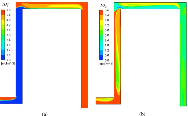
(a) (b)
Figure 3: Molar concentration of 𝐼𝑂3− on the centre-plane for Reynolds numbers of (a) 60 and (b) 300. Note that in case (a) the value is 0 on the first upward channel and 0.06 mol m-3 on the down flow, clearly indicating the swapping of the streams.
Due to the change in hydrodynamics for the two Reynolds numbers, the reaction behaviour is very different as shown in Figure 3, which shows the molar concentration of 𝐼𝑂3− on the centre-plane of the channel. At a Reynolds number of 60, reaction is slow because of the poor mixing. At the reactor inlet (bottom left-hand zone of Figure 3(a)), the 𝐼𝑂3− stream with its initial
occupies approximately half of the plane. After the first bend, however, the 𝐼𝑂3− stream disappears from the centre-plane as it moves either above or below it and then re-appears at the second bend. This is due to the twisting of streamlines shown in Figure 2. In contrast, at a Reynolds number of 300, the concentration of 𝐼𝑂3− is almost constant by the time the flow enters the first long straight channel on the right in Figure 3b.
13
(a) (b)
Figure 4: Sum of [𝐼2] + [𝐼3−] molar concentrations used in the segregation index at the channel
exit for Reynolds numbers of (a) 60 and (b) 300.
Figure 4 shows the values of [𝐼2] + [𝐼3−] at the micromixer exit used in the calculation of the
segregation index for the extremes of the Reynolds numbers considered. At Re = 300 the concentration of [𝐼2] + [𝐼3−] is very low and is almost constant (except for in the corners), which
demonstrates fast and effective micromixing. On the other hand, for Re = 60 the maximum concentration of [𝐼2] + [𝐼3−] is 100 times higher and there are large spatial differences in the
concentration field, which is representative of poorer micromixing performance. These concentration fields are coherent with the flow and Dean vortices shown in Figure 2. The number and intensity of Dean vortices clearly impact the structure of the formation of [𝐼2] +
[𝐼3−]: the four Dean vortices formed at a Reynolds number of 300 provide faster mixing than
for a Reynolds number of 60.
4.2 Segregation Index
The species concentrations simulated by CFD were used to determine the segregation index at the outlet of the channel. Figure 5 shows the calculated values compared with the experimental data. Error bars, which represent relative uncertainties of the experimental data, were estimated by the present authors. The main features of the experimental measurements are captured in the simulations. At Reynolds numbers of 200 and 300 the computational results are almost mesh independent as shown by the proximity of the three results. At a Reynolds number of 120 there is a small dependence on mesh size remaining, whereas at a Reynolds number of 60 the effect is still significant. No attempt was made to increase the mesh resolution to obtain a mesh
14
independent solution at the lowest Reynolds number as this is clearly not going to lead to a practical simulation approach.
Figure 5: Simulated segregation index as a function of Reynolds number for two mesh
resolutions and Richardson extrapolation with experimental data taken from Commenge and Falk (2011).
5. Results from the Striation Model
5.1. Striation Thickness Decay FunctionThe stretching experienced by material elements in the flow at the four Reynolds numbers (60, 120, 200 and 300) was calculated by tracking their position and deformation (Equations (23) and (24)) in the velocity field obtained from the CFD simulations. The mean stretching experienced by all the particles, 𝜆 ̅ (𝑡), was weighted by the inlet velocity of each fluid element
where 𝐧 is a normal vector to the micromixer inlet surface. An increasing number of elements were tracked until the mean value of the stretching for all the particles stabilised at a constant value. In this work, 1225 particles injected from each inlet were needed. Figure 6 shows that
𝜆 ̅ (𝑡) =𝜆(𝑡, 𝐗)𝐮(0, 𝐗) ∙ 𝐧̅̅̅̅̅̅̅̅̅̅̅̅̅̅̅̅̅̅̅̅̅ 𝐮(0, 𝐗) ∙ 𝐧
15
the mean stretching increases exponentially with time at faster rates as the Reynolds number of the flow in the micromixer increases. This is due to the formation of Dean vortices in the bends of the micromixer and consequently the increased amount of transverse flow at higher Reynolds numbers (see Figure 2), resulting in higher deformations.
The expression
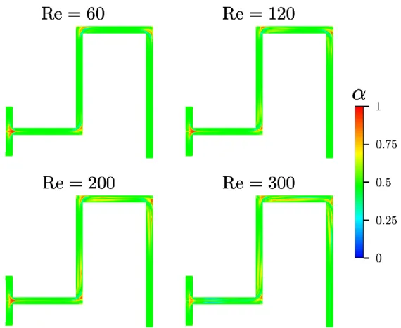
was fitted to the results in Figure 6 to be used later with the lamellar model described in Section 3. Equation (29) tries to capture the two components of the deformation promoted by the flow: simple shear (𝛾̇𝑐) and extension (Λ𝑐). The values of the simple shear and extensional components for the different Reynolds numbers studied are reported in Figure 7. It is evident that as the Reynolds number increases, the extensional component in the flow also increases. Figure 8 show the extensional efficiency of the flow,
at different Reynolds numbers, where 𝛾̇ is the shear rate and 𝜔 is the magnitude of the vorticity. When 𝛼 = 0 the flow produces no deformation (pure solid-body rotation). A value of 𝛼 = 0.5 corresponds to deformation due to simple shear and 𝛼 = 1 corresponds to a purely extensional flow. An analysis of the spatial distribution of the extensional efficiency in the channel reveals that extensional flow occurs at the bends and then increasingly in the straight section after the bend as the Reynolds number increases. The simple shear component also increases to some extent with Reynolds number but then starts to decrease after Re = 200. This change occurs with the onset of four Dean vortices instead of two at lower Reynolds numbers and signifies that extensional flow becomes dominant.
𝜆̅(𝑡) = √1 + 2(𝛾̇𝑐𝑡) + (𝛾̇𝑐𝑡)2𝑒Λ𝑐𝑡 (29)
𝛼 = 𝛾̇
16
Figure 6: Mean stretching as a function of time at different Reynolds number.
Figure 7: Values of fitting parameters for the striation thickness decay function at different
17
Figure 8: Extensional efficiency in the initial section of the micromixer at different Reynolds
numbers.
5.2. Mixing time calculation
For initial validation of the methodology, Equation (17) was adapted to describe the transport of a single non-reactive and passive chemical species in the flow in order to estimate the time required to achieve complete mixing at the molecular level. For these conditions, Equation (17) takes the form
which is solved for the initial condition
and the boundary conditions
𝜕𝑐 𝜕Γ= ( 𝑠0 𝑠) 2𝜕2𝑐 𝜕𝜉2 (31) Γ = 0: 𝑐 = 𝐻(𝜉) ∀𝜉 (32) Γ > 0: 𝜕𝑐 𝜕𝜉|𝜉=±1 2 = 0 (33)
18
The solution of Equation (31) with boundary and initial conditions (32) and (33)was obtained after 15 s for each flow condition and a discretization of the spatial variable with 2000 elements using a single core and 64 GB of RAM.
The index of segregation, 𝑋𝑆, was calculated from the non-dimensional evolution of the
variance of the concentration in the lamellar structures
Values of 𝑋𝑆 can vary between 1 (complete segregation) and 0 (complete mixing at the molecular level). The mixing time, 𝑡mix, was defined as the time necessary to obtain an
intensity of mixing 𝑋𝑆(𝑡mix) = 0.1%.
Figure 9 shows the evolution of 𝑡mix with the specific energy dissipation rate in the flow, 𝜖, for
the different Reynolds numbers. 𝜖 was determined from the CFD simulations by calculating the total viscous dissipation rate in the entire domain as
where 𝑉mixer is the volume of the micromixer and 𝐃 =1
2(∇𝒖 + (∇𝒖)
T) is the rate-of-strain
tensor. These results are in excellent agreement with experimental data obtained for the same micromixer geometry and various other geometries, where it has been observed that 𝑡mix∝ 𝜖−0.5 (Falk and Commenge (2010), Commenge and Falk (2011).
𝑋𝑆 =(𝑐 − 𝑐̅) 2 𝑐̅2 (34) 𝜖 = ∭ 2𝜇(𝐃: 𝐃) d3𝒙 𝑉mixer 𝜌𝑉mixer (35)
19
Figure 9: Mixing time as a function of the specific energy dissipation rate in the flow.
5.3. Segregation index from the Villermaux-Dushman test reaction
Equation (20) was solved with the average striation thickness decay function obtained by the Lagrangian approach to calculate the evolution of the segregation index, 𝑋𝑆. Figure 10 shows
the values obtained for 𝑋𝑆 at different Reynolds numbers in comparison with the experimental values of Commenge and Falk (2011). The lamellar model correctly predicts the rate of decay of the segregation index at higher values of Reynolds number but tends to over predict micromixing performance (underprediction of 𝑋𝑆) at the lower range of Reynolds. This over prediction of mixing is explained by the fact that the flow is fully segregated with little generation of fluid lamellae by engulfment of streams at the lower Reynolds numbers. This means that even if the fluid elements entering from each of the inlets are thinned down by deformation imposed by the flow, it does not result in the generation of inter-material area between the two fluids since the flow remains segregated. Indeed, the lamellar model is based on the generation of striations as the mechanism of mixing between the two inlet streams and is clearly not so well adapted for cases where the concentration fields are segregated.
20
Figure 10: Segregation index as a function of the Reynolds number: Lamellar model results
versus experimental data (data sets 1 and 2b of Commenge and Falk (2011)).
6. Conclusions
This work compares the performance of two methods – CFD simulations and a lamellar model – to simulate micromixing in a T-mixer with square bends in the laminar regime. Both models correctly reproduce previously published experimental data obtained with the Villermaux-Dushman micromixing test reaction. However, since the lamellar model relies on the generation of fluid lamellae, it does not perform so well at the lowest Reynolds number studied. A major conclusion of this work is that even for simple geometries and low Reynolds numbers, the direct simulation of micromixing using CFD can be very computationally expensive. Many 1000’s of CPU hours on 64 to 128 cores were required to obtain a solution in the current study. CFD simulations of the velocity fields in this type of geometry can be realised with modest computational cost, however huge computational costs are required in order to correctly resolve the concentration fields without numerical diffusion. The use of the lamellae-based micromixing model offers an attractive alternative to direct simulations. In this case, the flow field obtained by CFD allows the direct inclusion of the interface stretching and extension in the model enabling the reaction behaviour to be computed at a much-reduced computational
21
cost. In the current study, computational time required to resolve the concentration fields and reaction performance was less than one CPU hour on a single core. This lamellar model is therefore a promising solution to model fast chemical reactions in reactors with complex geometries in the laminar regime and for industrial applications. Indeed, since the model only requires the resolution of flow fields, much coarser computational grids than those required for the calculation of concentration gradients can be employed, thereby drastically reducing computational time.
Acknowledgements
The authors acknowledge the University of Sydney for providing High Performance Computing resources that have greatly contributed to the research results reported here
(http://sydney.edu.au/research_support). We thank Prof. Jean-Marc Commenge and
22
References
Assirelli, M., Wynn, E.J.W., Buialski, W., Eaglesham, A., Nienow, A.W., (2008). An extension to the incorporation model of micromixing and its use in estimating local specific energy dissipation rates. Ind. Eng. Chem. Res. 47, 3460-3469
Baccar, N., Kieffer, R., Charcosset, C., (2009). Characterization of mixing in a hollow fiber membrane contactor by the iodide–iodate method: Numerical simulations and experiments. Chem. Eng. J., 148, 517-524.
Baldyga, J., Bourne, J.R. (1984a). A fluid mechanical approach to turbulent mixing and chemical reaction, Part II Micromixing in the light of turbulence theory. Chem. Engng. Com., 28(4-6), 243-258.
Baldyga, J., Bourne, J.R. (1984b). A fluid mechanical approach to turbulent mixing and chemical reaction, Part III Computational and experimental results for the new micromixing model. Chem. Engng. Com., 28(4-6), 259-281.
Baldyga J., Bourne J.R., (1999). Turbulent mixing and chemical reactions, Wiley-Blackwell. Bothe D., Lojewski A., Warnecke H.-J., (2010). Computational analysis of an instantaneous chemical reaction in a T-microreactor. AIChE J., 56 (6), 1406-1415.
Bothe D., Lojewski A., Warnecke H.-J., (2011). Fully resolved numerical simulation of reactive mixing in a T-shaped micromixer using parabolized species equations. Chem. Eng. Sci., 66 (24), 6424-6440.
Commenge J.-M., Falk L., (2011). Villermaux–Dushman protocol for experimental characterization of micromixers. Chem. Eng. and Proc.: Proc. Intensif., 50(10), 979-990. Falk, L., Commenge, J.-M., (2010). Performance comparison of micromixers. Chem. Eng. Sci., 65, 405-411.
Fournier, M.-C., Falk, L., Villermaux, J., (1996). A new parallel competing reaction system for assessing micromixing efficiency–experimental approach. Chem. Eng. Sci., 51(22), 5053-5064.
Guichardon, P., Falk, L., (2000). Characterisation of micromixing efficiency by the iodide-iodate reaction system. Part I: experimental procedure. Chem. Eng. Sci., 55, 4233-4243. Guichardon, P., Falk, L., Villermaux, J., (2000). Characterisation of micromixing efficiency by the iodide-iodate reaction system. Part II: kinetic study. Chem. Eng. Sci., 55, 4245-4253. Kölbl, A., Kraut, M., Schubert, K., (2008). The iodide iodate method to characterise microstructured mixing devices. AIChE J., 54(3), 639-645.
23
Ottino, J.M., (1980). Lamellar mixing models for structured chemical reactions and their relationship to statistical models; Macro- and micromixing and the problem of averages. Chem. Eng. Sci., 35(6),1377-1381.
Ottino, J.M., Ranz, W.E. Macosko, C.W. (1979). A lamellar model for analysis of liquid-liquid mixing. Chem. Eng. Sci., 34(6), 877-890.
Palmer, D.A., Ramette, R.W., Mesmer, R.E., (1984). Triiodide ion formation equilibrium and activity coefficients in aqueous solution.J. Solut. Chem., 13(9), 673-682.
Rahimi, M., Azimi N., Parvizian F., Alsairafi A.A., (2014). Computational Fluid Dynamics modeling of micromixing performance in presence of microparticles in a tubular sonoreactor. Comp. Chem. Eng., 60, 403-412.
Ranz, W.E., (1979). Applications of a stretch model to mixing, diffusion, and reaction in laminar and turbulent flows. AIChE J., 25(1), 41-47.
Reckamp, J.M., Bindels, A., Duffield, S., Liu, Y.C., Bradford, E., Ricci, E., Susanne, F., Rutter, A., (2017). Mixing performance evaluation for commercially available micromixers using Villermaux−Dushman reaction scheme with the interaction by exchange with the mean model. Org. Process Res. Dev., 21, 816-820.
Roache, P.J., (1998). Verification and validation in computational science and engineering, Hermosa Publishers, Albuquerque, USA.
Santos R.J., Dias M.M., Lopes J.C.B., (2012). Mixing through half a century of chemical engineering. In: Single and Two-phase Flows on Chemical and Biomedical Engineering, Bentham Science, pp. 79-112.
Schikarski T., Peukert W., Avila M., (2017). Direct numerical simulation of water–ethanol flows in a T-mixer. Chem. Eng. J., 324, 168-181.
Schikarski T., Trzenschiok H., Peukert W., Avila M., (2019). Inflow boundary conditions determine T-mixer efficiency. React. Chem. Eng., 4, 559-568