Censored Regressors and Expansion Bias

MIT Sloan School of Management

Working Paper 4451-03

December 2003

Censored Regressors and Expansion Bias

Roberto Rigobon, Thomas M. Stoker

© 2003 by Roberto Rigobon, Thomas M. Stoker. All rights reserved. Short sections of text, not to exceed two paragraphs, may be quoted without explicit permission, provided that full credit including © notice is given to the source.

This paper also can be downloaded without charge from the Social Science Research Network Electronic Paper Collection:

Censored Regressors and Expansion Bias

Roberto Rigobon Thomas M. Stoker

November 2003

Abstract

We show how using censored regressors leads to expansion bias, or estimated e¤ects that are proportionally too large. We show the necessity of this e¤ect in bivariate regression and illustrate the bias using results for normal regressors. We study the bias when there is a censored regressor among many regressors, and we note how censoring can work to undo errors-in-variables bias. We discuss several approaches to correcting expansion bias. We illustrate the concepts by considering how censored regressors can arise in the analysis of wealth e¤ects on consumption, and on peer e¤ects in productivity.

1. Introduction

When the values of the dependent variable of a linear regression model are censored, the OLS estimates of the regression coe¢ cients are biased. This familiar fact is a standard lesson covered in textbooks on econometrics. It has stimulated a great deal of work on consistent estimators of coe¢ cients when there is a censored dependent variable.

In view of this, it seems surprising that very little attention has been paid to implications of censoring of an independent variable, or regressor, in estimation of a linear model. Indeed, it would seem that researchers encounter censored regressors as often or even more often than situations of censored dependent variables. Consider how often variables are observed in ranges, including unlimited top and bottom categories. For instance, observed household income is often recorded in increments of one thousand or …ve thousand dollars, but would have a top-coded response of, say, “$100,000 and above.” Here we are interested in what di¤erence it makes if we estimate a regression with the top-coded income data when the correct speci…cation has income level (no top coding) as the appropriate regressor.

We show that using a censored regressor results in expansion bias in OLS estimates of regression coe¢ cients, namely, estimated e¤ects will be too large in absolute value.1 For instance, if income is

Sloan School of Management, MIT, 50 Memorial Drive, Cambridge, MA 02142 USA. We have received valuable comments from Vincent Hogan, Dale Jorgenson and Whitney Newey.

1_{Expansion bias is the opposite of attenuation bias, familiar from problems such as errors-in-variables or simple censored}

top-coded (or bottom-coded, or both), a positive income e¤ect will be overestimated. This fact is straightforward to show, and several approaches for correcting it can be proposed.

When there are many regressors, the bias associated with using a censored regressor is more com-plicated, but some useful understanding of it can be developed. We supplement general derivations with exact formulae for the case when all regressors are normally distributed. We study an interesting side issue, which is what bias occurs when a regressor that is measured with error is also censored. In that case the two sources of bias work in opposite directions, and can cancel each other out. We develop this relationship as well to show some useful trade-o¤s in these bias problems.

We note at least three approaches for correcting expansion bias in empirical work. When the form of the distribution of the regressors is unknown, there is a semiparametric approach that appears to be the most e¢ cient method.

We discuss how censored regressors can arise in two speci…c application areas; the estimation of wealth e¤ects on consumption, and the estimation of peer group e¤ects on productivity. Our discussion is intended to give concrete illustration to the ideas, and we plan to carry out applications of these kinds as part of future research.

Expansion bias from censored regressors is a straightforward problem, but ignoring that problem can lead to substantial mismeasurement of e¤ects. Section 2 shows how expansion bias arises, and considers several related topics including what can be said when there are many regressors. Section 3 discusses corrections for expansion bias, Section 4 discusses the application areas, and Section 5 gives some concluding remarks.

2. Censored Regressors and Expansion Bias

2.1. The Basic Problem

We start with bivariate regression to see the simplest form of expansion bias. Suppose that the true model is

yi = + xi+ "i i = 1; :::; n (1)

where xi is the (uncensored) regressor and "i is the disturbance. We assume that the distribution of

(xi; "i) has …nite second moments and obeys E ("ijxi) = 0. Suppose that xceni denotes the censored

version of xi with bottom-coding and top-coding, as

xcen_i = xi 1 xi + + 1 xi< + + 1 +< xi (2)

where ; + are scalars, < +. In words, xcen

i is xi when in the range xi +, but is equal to

the respective lower limit or upper limit + when xi falls out of that range. The question of interest

is what happens when we use xcen_i to estimate ; namely if we estimate the model

yi = a + bxceni + ui i = 1; :::; n; (3)

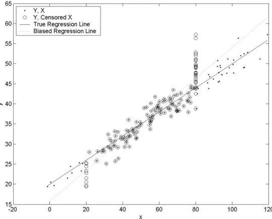
A picture makes the answer clear. Figure 1 shows a scatterplot of data without censoring of the regressor. The small circles are the resulting data points when the regressor is censored at upper and lower bounds. The estimated regression using the censored regressor clearly has a steeper slope that the one using the uncensored regressor, because of the “pile-up” of observations at each limit. This is what we call expansion bias. Moreover, it is clear that expansion bias would result if there was only one-sided censoring (top-coding or bottom-coding only); that each censoring limit contributes to the amount of expansion bias.

A more formal analysis re‡ects these features as well. We begin by stating the conclusion as: Proposition 1. Provided that 0 < Pr x < + Pr x > + < 1, we have

plim ^b = (1 + ) (4)

where > 0.

The proof of Proposition 1 is direct, and given in the following subsection (it may be skipped in a quick reading). It shows that the relative bias is

= + +; (5)

where and + are positive terms that arise from censoring at the bottom limit and the top limit respectively, exactly in line with Figure 1. This is the main result on censoring with bivariate regression. After the proof, we show the size of the bias when the uncensored regressor is normally distributed, and then we develop the bias in the context of many regressors in Section 2.2.

2.1.1. Proof of Proposition 1

Begin by de…ning the parts of xi that are omitted by censoring.

x_i = xi 1 xi< and xi+= xi + 1 +< xi ; (6)

so that the true model (1) appears as

yi= + xceni + xi + x +

i + "i i = 1; :::; n (7)

The omitted variable bias formula then gives

plim ^b = 1 + + + (8)

where , + are the auxiliary coe¢ cients from omitting x_i , x+_i respectively, namely = Cov (x ; x

cen₎

V ar (xcen₎ and

+₌ Cov (x+; xcen)

Consider …rst, and assume that Pr x < > 0 (since if Pr x < = 0, then = 0). We have

Cov (x ; xcen) = E (x xcen) E (x ) E (xcen)

= E x 1 x < 0 E (x ) E (xcen) = E (xcen) E (x )

= E xcen E (x )

(10)

Each of the expectations E xcen _{and E (x ) is an integral with nonpositive integrand, and each}

integrand is strictly negative over a range of positive probability. Therefore, each of the expectations is strictly negative, and their product Cov (x ; xcen) is strictly positive. We conclude that

= Cov (x ; x

cen₎

V ar (xcen₎ > 0 (11)

so that omitting x_i results in expansion bias.

Similarly for +, we assume Pr x > + > 0, and derive

Cov x+; xcen = E + xcen E x+ (12)

Here, each of the two expectations is an integral with nonnegative integrand, and each integrand is strictly positive over a range of positive probability. Therefore, each of these expectations is strictly positive, as is their product Cov (x+; xcen), and we conclude that

+₌ Cov (x+; xcen)

V ar (xcen₎ > 0 (13)

so that omitting x+_i also results in expansion bias. This shows Proposition 1, where = + +.2

2.1.2. Expansion Bias with a Normal Regressor

The expansion bias depends on various expectations over truncated distributions. Assuming a particular distributional form will often allow the bias to be computed directly. In econometrics, the most familiar formulae for truncated and censored expectations are from a normal distribution. In this section we illustrate the bias assuming that the uncensored regressor x is normally distributed with mean _x and variance 2_x. To examine the bias at di¤erent levels of censoring, we can parametrize using the censoring limits , +, or equivalently, the probabilities of censoring p = Pr x < , p+= Pr x > + . We choose the latter, because of a sort of ‘scale free’intuition.

2

It should be noted that (or +) is slightly larger than the bias term that would arise if there was only censoring of low values (or high values). That bias term is in the form (11) (or (13) respectively) with the same numerator but slightly larger denominator (since xcen is only censored on one side). More on this in the discussion of Figure 2.

The bias formulae themselves are complicated and do not admit to obvious interpretation. Because of that, we give a brief derivation and show the formulae in Appendix A. Here we illustrate the bias graphically.

Figure 2 gives two depictions of expansion bias. The solid line displays the two-sided bias of (5) under the assumption of symmetric censoring, with the same probability p = p+ p of censoring in the high and low region, and is plotted against the total probability of censoring 2p. The dashed line is the expansion bias from one-sided censoring, or top-coded data, which is plotted with the same total censoring probability. For instance, plotted over 2p = :2 is the two-sided bias from censoring 10% in each tail, and the one-sided bias from censoring 20% in the upper tail. For comparison, the diagonal (2p; 2p) is included as the dotted line.

We see that the bias is roughly linear in 2p for low censoring levels, up to around 30% of the data censored. After that the bias rises nonlinearly, but a bias that doubles the coe¢ cient value involves a lot of censoring; 60% or more of the data.

The two-sided bias is greater than the one-sided bias over the whole range of probabilities. So, in this sense, censoring on both sides induces more than twice the bias of censoring on one side only. This is likely due to the fact that with two-sided censoring, the censored points are in two separated groups and therefore have more in‡uence on the estimated regression.

2.2. Expansion Bias and Several Regressors

We now study expansion bias when there are one or more regressors. We extend the model (1) to include a k-vector or regressors zi as

yi= + xi+

0

zi+ "i i = 1; :::; n (14)

where we assume that the distribution of xi; z0i; "i is nonsingular, has …nite second moments and

obeys E ("ijxi; zi) = 0. Again, we are interested in what happens when xceni is used instead of xi; so if

we estimate the model

yi = a + bxceni + c

0

zi+ ui i = 1; :::; n; (15)

then how are the OLS coe¢ cients ^a; ^b; ^c biased as estimators of ; ; ?

We can develop a deeper understanding of expansion bias by viewing the OLS estimation in (15) as a pooled regression. As discussed further in Section 3, no bias is generated by observations that are not censored, or ‘truncated’ observations. To use this fact, it is valuable to de…ne the following approximation device: x( )_i = 8 < : xi+ (1 ) if xi < xi if xi + xi+ (1 ) + if + < xi (16)

We write the true model (14) in terms of x( )_i , and approximate the estimation of (15) as a pooled regression of the three samples, the ‘low censored’ with xi < , the ’truncated’ with xi +,

and the ‘high censored’with +< xi. For ‘low censored’observations, we have

yi = + 1

1

+ + 1 1 x( )_i + 0zi+ "i ; if xi< ; (17)

for ’truncated’observations we have

yi= + x( )i +

0

zi+ "i ; if xi + (18)

and for ’high censored’observations we have yi= + + 1

1

+ + 1 1 x( )_i + 0zi+ "i ; if + < xi (19)

Denote the OLS coe¢ cients from regression yi on a constant, x( )i and zi as ^a( ); ^b( ); ^c( ). The

bias in those estimates is given as

plim 0 @ ^ a( ) ^_b( ) ^ c( ) 1 A 0 @ 1 A = [ ] 1 2 6 6 4p 0 B B @ 1 1 1 ₁ 0 1 C C A + p+ + 0 B B @ + ₁ 1 1 ₁ 0 1 C C A 3 7 7 5 (20) where p = Pr x < is the probability of ‘low censoring,’p+= Pr x > + is the probability of ’high censoring,” and

= E 1; x( ); z0

0

1; x( ); z0 = p + (1 p p+) trun+ p+ + ; (21) where ; trun; + are the conditional second moment matrices over the ‘low censoring’ region x < , the truncated region xi +, and the ‘high censoring’ region x > +, respectively.

The bias (20) is a matrix-weighted average of the biases in the low and high censoring regions; with expansion bias terms 1 1 from each region. As _{! 0, these bias terms explode, and so for the} approximation device to be useful, we must verify that the weights ; + shrink at the same rate.

This is easy to do. By spelling out the moments as _{! 0, it is immediately clear that} E y; 1; x( ); z0 0 y; 1; x( ); z0 _{! E} y; 1; xcen; z0 0 y; 1; xcen; z0 (22) so that ₀ @ ^ a( ) ^_b( ) ^ c( ) 1 A ! 0 @ ^ a ^_b ^ c 1 A (23)

and

! E 1; xcen; z0

0

1; xcen; z0 : (24)

The bias components can be computed directly, for instance

p+ + 0 B B @ + ₁ 1 1 ₁ 0 1 C C A = p+ (1 ) 0 @ + x + M+ xx +x + + (1 ) + +x + M_xz+ +_z + 1 A ! p+ 0 @ + x + + + x + M_xz+ +_z + 1 A B+ (25)

where ‘+ ’indicates expectation over the ‘high censoring region’; namely +_{x = E x j x >} + , +_z = E z j x > + , M_xx+ = E x2 _{j x >} + , M_z+ = E zz0 _{j x >} + ; and the weight + shrinks to 0 because the variance of x( ) shrinks to 0 over that region. By the symmetries in the formulae, we have

p 0 B B @ 1 1 1 ₁ 0 1 C C A = p (1 ) 0 @ xM_{xx x} + (1 ) _x M_{xz z} 1 A ! p 0 @ x _x M_{xz z} 1 A B (26)

So, as above, the overall bias in ^a; ^b; ^c0 is the sum of biases generated by the low and high censoring region, plim 0 @ ^ a ^ b ^ c 1 A 0 @ 1 A = 1 0 @ p _x + p+ +_x + p _x + p+ + +_x + p M_{xz z} + p+ _M+ xz +z + 1 A = B + B+_{: (27)}

where B and B+ are de…ned in (25) and (26).

We can easily interpret these formulae in the ‘no correlation’ case. Suppose _z = 0 and that z is mean independent of x. Then _z = +_z = M_xz = M_xz+ = 0, and is block diagonal (partitioned according to (1; xcen_{); z). Consequently, there is 0 bias in the z coe¢ cient ^c, and ^a; ^b behave as}

though z were not in the equation for estimation. If further, E (xcen_{) = 0 (which implies < 0 <} +_),

then we have

and

plim ^b = p x + p

+ + +

x +

V ar (xcen₎ : (29)

The bias in the intercept ^a consists of a negative ‘low censoring’term and and a positive ‘high censoring’ term. For ^b there is positive expansion bias term from both low and high censoring (as consistent with Proposition 1). In a ‘symmetric censoring’ case with p = p+; = +, and _x = +_x, the intercept bias is exactly o¤set, plim ^a = 0. The slope ^b contains equal expansion bias terms from low and high censoring; plim ^b = 2 p+ + +_x + V ar (xcen).

For the case with correlation, the exact bias formulae are too complex to admit clear interpretation. However, we can learn from expanding the bias in terms of the censoring probabilities, as follows. Here we examine the ‘high censoring bias’ B+, and an analogous development can be carried out for B . Suppose there is a single variable z with _z= 0, and we now take _x= 0. Now, through a very tedious calculation, the bias B+ _{can be written as terms linear in p}+ _{and terms of higher polynomial order in}

p+. Dropping the higher order terms, we have

B+= p + MzzMxx (Mxz)2 0 B @ MzzMxx (Mxz)2 +x + Mzz + +x + Mxz Mxz+ + +z Mxx Mxz+ + +z Mxz + +x + 1 C A (30)

where Mxx = E x2 ; Mxz = E (xz) and Mzz = E z2 are unconditional (and uncensored) second

moments. For p+ small, this should be a very good approximation (since (p+)k, k 2 is much smaller than p+). Let x =pMxx; z =pMzz denote the unconditional standard deviations of x and z and

let _xz denote their correlation coe¢ cient.

The approximate bias term for the intercept ^a is p+ +_x + ,which is the same form as in (28). For ^b and ^c, the biases are:

plim ^b _ p+ + +_x + _xz x z M_xz+ + +_z (31) and plim ^c _ p+ x z M_xz+ + +_{z xz} + +_x + (32)

where the positive proportions are from (30) and are therefore approximate.

To interpret these terms, suppose that x and z are positively correlated overall ( _xz > 0), positively correlated within the ‘high censored’region (within covariance C_xz+ > 0), and that + > 0. Given this, we have + +_x + > 0 and M_xz+ + +_z = C_xz+ + +_x + +_z > 0. So, the approximate biases are each di¤erences of positive terms. They can be interpreted as follows. Since x and z are positively correlated, in OLS estimation z will proxy some of the role of the censored values of x. Therefore, for ^_{b, we see that (31) consists of the positive expansion bias term of (29), less a positive term due to z’s}

Bias of: Correlation Truncation -90% -50% 0% 50% 90% ba 0.1% 0.1% 0.1% 0.1% 0.1% 1% bb -0.4% 0.7% 0.8% 0.7% -0.4% bc -0.4% -0.1% 0.0% 0.1% 0.4% ba 3.3% 4.2% 4.3% 4.2% 3.3% 20% bb -11.5% 12.3% 14.5% 12.7% -10.3% bc -8.0% -2.6% -0.2% 2.3% 7.7% ba 7.2% 11.9% 12.5% 12.0% 7.4% 40% bb -23.2% 26.1% 32.2% 27.2% -21.4% bc -14.9% -6.5% -0.5% 5.6% 14.5% ba 14.2% 29.7% 32.3% 30.1% 14.3% 60% bb -27.2% 52.2% 65.9% 54.2% -25.6% bc -20.2% -11.7% -0.9% 10.3% 19.9%

Table 1: Coe¢ cient Biases: Two Regressors with One Censored.

role as a proxy for the censored values of x: Similar terms arise for ^c in (32) in the reverse positions; a positive bias arises because z proxies the censored values of x, less a term arising from the expansion bias of the coe¢ cient for the uncensored x values.

It is interesting to note that the net biases can go either way depending on the correlation between x and z. For a small correlation, the expansion bias in ^b will be evident, and a negative bias in ^c arises in response to that. For a large correlation, the positive expansion bias in ^b can be wholly reversed, and with a positive bias arising for ^c. In that case, it appears that z is doing a better job of proxying for x than the censored xcen _is.

To clarify the intuition of the previous derivation we performed a Monte Carlo exercise. We assumed that x; z and " are normally distributed,3 and computed OLS estimates for di¤erent degrees of (top-coding) censoring and di¤erent correlations between x and z. Summary results are given in Table 14

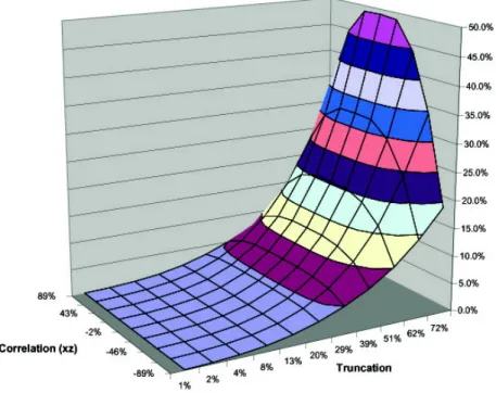
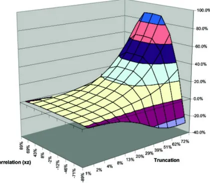
and the full results are displayed in Figures 3 to 5.

As can be seen in the Figure 3 and Table 1, the bias on the intercept ^a is always positive (for top-coding) and it is sizeable. For example, if 20 percent of the observations are censored there is a bias of roughly 4 percent. For the coe¢ cient ^b of the censored regressor xcen, the results are in line with the intuition we developed before. Namely, at low and moderate levels of correlation between x and z, there is a clear expansion bias, but as the correlation becomes high, the bias turns negative. The highest bias occurs at zero correlation, and it decreases with as absolute value of the correlation increases. For the coe¢ cient ^c of the other regressor z, bias and correlation have a monotone relationship. Positive bias arises for positive correlation and negative bias for negative correlations, with larger levels of censoring implying larger biases in absolute terms. This also is in line with the intuition above. In any case, we feel these results suggest that the biases introduced by the censoring of a regressor can be large and

3_{We set = 1, = 0:5, and = 0:75, took the variances of x and z to be the same and equal to half the value of the}

variance of ".

4_{In line with (15), ^ais the estimated intercept, ^bis the estimated coe¢ cient on the censored variable x and ^cis the}

economically signi…cant.

2.3. Expansion Bias and Errors-in-Variables

We close this section with a curiosity about censoring regressors that are measured with error. Errors-in-variables cause attenuation bias whereas censoring regressors causes expansion bias, the opposite. So it is natural to consider correcting for errors-in-variables by censoring the variable measured with error.

Consider the bivariate model

yi= + wi+ "i; i = 1; :::; n (33)

where

xi = wi+ i (34)

and "i, i and wi are mutually uncorrelated: If we estimate

yi = a + b xi+ i i = 1; :::; n; (35)

then we have the standard result that

plim ^b = (1 ) ; = Var ( )

Var (x): (36)

However, if we further censor x as above, and estimate

yi = a + bxceni + ui i = 1; :::; n; (37) then we have plim ^b = (1 ) (1 + ) (38) Provided (1 ) (1 ) = 1, or = 1 (39)

then the errors-in-variables bias will have been corrected by the censoring.

It is not clear how practically useful this fact is, since to know how much to censor would require knowing how much error variance there is (and then it could be corrected directly). But we …nd it an interesting connection, and it suggests some other questions. Does correcting a certain attenuation bias require a great deal of censoring or very little? Is one of these bias problems of a di¤erent order of magnitude than the other?

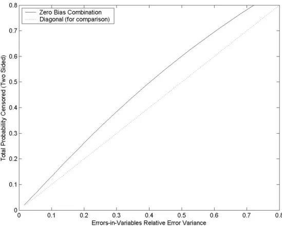
Figure 6 sheds light on these questions for a normal regressor. It shows the level of censoring required to correct each level of attenuation bias. Speci…cally, it is assumed that there is two-side symmetric censoring (p low and p high censoring), and it plots the total censoring probability 2p against the relative error variance underlying the zero bias condition (39). It shows that the probability of

censoring 2p needs to be a larger than the error variance but not a great deal larger. For instance, slightly less than 40% total censoring would be needed to correct the bias implied by 30% relative error variance. In any case, the impact of censoring a certain percentage of the data can be thought of a slightly smaller than the impact of an error variance of the same level, in the opposite direction.

In any case, it is clear that errors-in-variables bias can be counteracted by the censoring the regres-sor. This does raise questions about survey design. Suppose that a variable is measured with error and that error is likely higher for the top range of the variable - for example, hours spent in tra¢ c, gallons of beer consumed, etc. In this circumstance it is possible some degree of top-coding would make sense as part of survey design. In any case, there may be some practical impact to the interplay of censoring with errors-in-variables.

3. Correcting Expansion Bias

There are at least three broad approaches to correcting expansion bias that are useful to discuss. The …rst approach is to focus on the distribution of the regressors, assuming a speci…c form that allows the bias terms to be identi…ed. The bias terms could then be estimated (or simulated), and the OLS coe¢ cients adjusted by the bias estimates. This approach has the usual proviso about distributional assumptions in econometric work – namely there is usually not a great deal of guidance as to what structure should be assumed, especially in multivariate settings. However, it is worthwhile to note that since the regressors are observed, assumptions on their distributional structure are (potentially) testable. For instance, to validate the assumption that the regressors are multivariate normal, one could apply goodness-of-…t tests to check whether the censored regressor is distributed as a censored univariate normal.

The second approach is to eliminate the problematic data. That is, estimation can be done on the truncated sample with < xcen_i < +, where all observations with censored data have been deleted from the sample. As we noted in Section 2.2, the OLS estimators from the truncated sample will be unbiased and consistent estimators of the true coe¢ cients. Because the censored data is informative, one would expect an e¢ ciency loss from this approach, but it is so simple to do that it is probably good empirical practice to always compute the estimates from the truncated sample for comparison. This approach also illustrates an important di¤erence between the censoring of a regressor and the more familiar problem of censoring a dependent variable. Dropping all censored observations of a dependent variable does not avoid the bias in OLS coe¢ cients.

The third approach is to augment the speci…cation of the regression equation to remove the source of the bias. Consider the case of many regressors. The true model is

yi = + xceni +

0

zi+ x_i + x+_i + "i i = 1; :::; n (40)

where

x_i = xi 1 xi < and x_i+= xi + 1 +< xi : (41)

of x and x+ that are correlated with the included regressors; as in yi = + xceni +

0

zi+ E x jxcen = xceni ; z = zi (42)

+ E x+_jxcen= xcen_i ; z = zi + ei

where ei "i E (x jxcen= xceni ; z = zi) E (x+jxcen = xceni ; z = zi) is uncorrelated with xcen and

z.

Let’s examine these correction terms in a bit more detail. First, we have

E x jxcen= xcen_i ; z = zi = 0 if xceni 6= (43)

f (zi) if xceni =

and

E x+_jxcen= xcen_i ; z = zi = 0 if xceni 6= + (44)

f+(zi) if xceni = +

So, the terms are nonzero only for the censored observations, but for those points, they are functions of zi that are determined by the joint distribution of x and z. As before, if we assume a speci…c form

for the joint distribution of x and z, we could derive and/or estimate the functions f ( ) and f+( ). Treating those functions as unknown, we have a fully semiparametric model

yi= + xceni +

0

zi+ f (zi) d_i + f+(zi) d+_i + ei, i = 1; ::; n (45)

where d_i 1 xcen

i = and d+i 1 xceni = + indicate the censored points. As long as p > 0,

p+ > 0, 1 p p+> 0, the model is identi…ed. In heuristic terms, we can identify , and with the truncated data, the function f (zi) from yi

0

zi for the low censored points, and the

function f+_(z

i) from yi +

0

zifor the high censored points. The model (45) is is very similar

to partially linear models as originally studied by Robinson(1988), and estimation can be approached by series expansion, within-di¤erencing or a variety of other techniques. We do not go into the details of these methods here, but we will analyze them in subsequent research.5

It is useful to consider whether there are ‘quick-…x’methods to recommend for empirical practice. Since f (zi) and f+(zi) are unknown functions, an initial idea is to approximate them by linear

functions. This amounts to allowing the regression parameters to vary between the truncated data, the low censored data and the high censored data. This is accomplished by adding d_i , d_i zi, d+_i , d+_i zi

to the list of regressors. This should help remove some of the bias in the coe¢ cients of 1; xcen_i and zi.

Are linear approximations likely to be good in this problem? The functions f (zi) and f+(zi) are

unknown and so there is no real substitute for a fully semiparametric approach to estimating them. However, it is useful to return once again to the case of a multivariate normal distribution and see how

5

Yatchew (2003) contains coverage of partially linear models and many references. Schmalensee and Stoker (1999) analyzes U.S. gasoline demand using partially linear models, with bivariate nonparametric structure.

‘linear’ f (zi) and f+(zi) are. Taking z to be a single variable for simplicity, under the assumption

that (x; z) are joint normal, f (zi) and f+(zi) are easily derived. We present the formulae in Appendix

A.

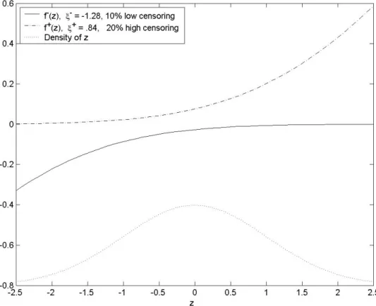
Figure 7 plots these functions assuming that x and z are standard normal, with a correlation of .5. The function f (zi) is based on 10% low censoring, and f+(zi) is based on 20% high censoring.6

The functions are not wildly nonlinear over the substantive range of z density, but they are not linear either. So here some nonlinear terms would be necessary for a good approximation. In general, a semiparametric method would allow more arbitrary shapes to be captured, and one could perform tests for the function shapes implied by joint normality.

4. Situations where Censored Regressors are Endemic

This paper is our …rst writing on censored regressors, and we are in the process of developing appli-cations where censored regressors are prevalent and where empirical …ndings may have been greatly impacted by their presence. We now describe some of the areas we plan to study as part of future research, to give more concrete illustration to the issues we have been discussing.

4.1. The E¤ects of Wealth on Consumption

In recent years, many developed countries have witnessed tremendous expansions in consumption ex-penditures at the same time as substantial increases in household wealth levels.7 _{This has fueled great}

interest in the measurement of the e¤ects of wealth on consumption decisions.

Consider …rst the issues associated with studying how consumption reacts to changes in …nancial wealth, say with a stylized model:

Ci = + IN Ci+ F Wi+ "i i = 1; :::; n (46)

where Ci is consumption, IN Ci is income and F Wi is a measure of …nancial wealth, such as the value

of stock and bond holdings. Now, it is very common that income is top-coded, producing the kind of censored regressor bias that we have discussed. But also, measures of …nancial wealth are often bottom-coded re‡ections of actual wealth, because of problems in measuring or capturing debt levels. That is, using only positive components of wealth, such as actual stock and bond holdings, generates a censored regressor problem of the same style as that generated by top-coded income. Since income

6_{We choose di¤erent values to illustrate how the shapes of the functions can vary. It is easy to verify that the}

same amount of low and high censoring (here = +) gives the functions as negative re‡ections of one another, f ( z) = f+_{(z) :}

7

During the 1990’s there were multiyear expansions in consumption in the US and the UK (among others). During the same time, the total wealth of Americans grew more than 15 trillion dollars, with a 262% increase in corporate equity and a 14% increase in housing and other tangible assets (see Poterba (2000) for an excellent survey). Housing prices increased in both countries as well.

and measured wealth tend to be positively correlated, wealth (and income) e¤ects will tend to be overestimated.

In fact, published estimates of the elasticity of consumption with regard to …nancial wealth seem large. With aggregate data, estimates in the range of 4% but up to 10% can be found, varying with the type of asset included and the time period under consideration.8 With individual data, estimates tend to be larger,9 such as 8%. In any case, we plan to investigate whether the censored character of income and …nancial wealth can help account for the magnitude of these estimates.

These issues are greatly exacerbated when one adds consideration of housing wealth, as in.

Ci = + IN Ci+ F Wi+ HWi+ "i i = 1; :::; n (47)

where HWi is housing wealth. Even when housing wealth is accurately measured, the censoring of

income and/or …nancial wealth will cause the e¤ect of housing wealth to be overestimated. In fact, estimates of the marginal propensity to consume out of housing wealth elasticity are in the range of 18%, which again seems quite large.10 It would be interesting to understand how much of this e¤ect could be due to censored regressor problems.

It is worth mentioning that estimates of wealth e¤ects are of substantial interest to economic policy. A key issue of monetary policy is how much aggregate demand is a¤ected by changes in interest rates. In addition to the direct e¤ects on consumption, it is obvious that interest rates will a¤ect housing wealth as well as …nancial wealth. A substantial impact of wealth on consumption, either through enhanced borrowing or cashing out of capital gains, will be a big part of whether interest rates are e¤ective or not. In any case, understanding these connections is crucial for the design of e¤ective monetary policy.11

4.2. Minimum Wage and Peer E¤ects

Here we consider how peer e¤ects in productivity are studied, as in Borjas (1994), Card et. al. (1998), and others. In this work, it is typical to use the average wage of the peer group as a proxy for the ability level of the peer group. This introduces error-in-variables structure in the standard way. However, if minimum wage rules are binding for some groups, then there is a censored regressor problem. As

8_{Laurence Meyer and Associates (1994) …nd an elasticity of 4.2 percent, Brayton and Tinsley (1996) …nd 3 percent,}

Ludvigson and Steindel (1999) estimate an overall elasticity of 4 percent (as well as some estimates as high as 10 percent).

9_{Using the PSID, Parker (1999) concludes that the elasticity of household expenditures to household net worth is}

approximately 8 percent (although the PSID has few households with large …nancial wealth holdings). Juster, Lupton, Smith and Sta¤ord (1999) and Starr-McCluer (1999) …nd slightly smaller coe¢ cient, but still larger than the ones obtained from aggregate data.

1 0_{See Aoki, et. al. (2002a, 2002b) and Attanasio, et. al. (1994), among others. Somewhat smaller estimates are given}

in Engelhardt (1996) and Skinner (1996).

1 1

See Muellbauer and Murphy (1990), King (1990), Pagano (1990) Attanasio and Weber (1994) and Attanasio et. al. (2003), for various arguments on the connection between consumption and housing prices. In terms of whether assets prices should be targeted as part of monetary policy, see Bernanke and Gertler (1999,2001), Cecchetti et. al. (2000) and Rigobon and Sack (2003).

discussed in Section 2.3, the ‘censored regressor’bias will be in the opposite direction to the "errors-in-variables’bias.

For concreteness, consider the model:

Yi= + Hi+ "i; i = 1; :::; n (48)

where Yi is the variable of interest12 and Hi stands for ability of the individual of the peer group.

Suppose Wi is the true wage of the peer group that is correlated with ability, as in

Wi= Hi+ i (49)

"i and i are standard innovations, assumed to be uncorrelated.

Now, if true wage Wi is observed and used as a proxy for ability Hi, as in

Yi = + Wi+ i; (50)

then there is a pure errors-in-variables problem. Proper instruments could be used to obtain consistent estimates. However, suppose that there is a minimum wage constraint, so that observed wage is in fact

W_icen = W 1 [Wi < W ] + Wi 1 [Wi W ] (51)

In this situation, the regression

Yi = + Wicen+ i; (52)

has errors-in-variables and a censored regressor. As discussed in Section 2.3, the attenuation bias from errors-in-variables can be counteracted by the expansion bias from the censored regressor.

5. Conclusion

The fact that censored regressors generate expansion bias was a big surprise to both authors. We noticed the phenomena in some simulations, and were able to understand the source pretty easily. In fact, it is a completely straightforward point, as Figure 1 can be explained to students with only rudimentary knowledge of econometric methods. Nevertheless, we don’t feel that it is a minor problem for practical applications. Quite the contrary, we feel that problems of censored regressors are likely as prevalent or more prevalent than problems of censored dependent variables in typical econometric applications.

We feel that we were able to make some progress in understanding the structure of expansion bias. Sure, the ‘many regressor’formulae are complicated – in what problem are they easy? – but we were

1 2

Examples of Yiinclude own wages, hours worked, decisions of …nancing, decisions of participation in …nancial markets

or labor markets, etc., or any decision that is a¤ected by peer considerations. As with out discussion of consumption, applications would include control variables, which we abstract from for this discussion.

able to see how the censoring issues transmit across regressors. We were able to get a sense of the severity of the biases using formulae and simulations from normal distributions, and a side comparison to the biases that arise from errors in variables.

But the real value of this material will be decided by how well expansion bias can be isolated in actual applications. Here, we are quite hopeful. There is a correction method which is easy to implement, understand and interpret – drop the censored points and see what happens. And, there is a straightforward semiparametric approach for using all the data, including the censored points. While we are not yet at the point of having a well tried "set of instructions" for implementing the semiparametric approach, we expect to generate one as a byproduct of doing applications ourselves.

References

[1] Aoki, K., J. Proudman and G. Vlieghe (2002a) “House prices, consumption, and monetary policy: a …nancial accelerator approach” Bank of England Quarterly Bulletin.

[2] Aoki, K., J. Proudman and G.Vlieghe (2002b) “Houses as collateral: has the link between house prices and consumption in the UK changed?’, Economic Policy Review Vol. 8 (1), Federal Reserve Bank of New York,

[3] Attanasio, O., L. Blow, R. Hamilton, and A. Leicester (2003) “Consumption, House Prices, and Expectations” Institute for Fiscal Studies, Mimeo.

[4] Attanasio, O., and G. Weber (1994) “The UK Consumption Boom of the late 1980s: aggregate implications of microeconomic evidence”in The Economic Journal, Vol. 104, Issue 427, November, pp 1269-1302.

[5] Bernanke, B., and M. Gertler, “Monetary Policy and Asset Price Volatility,”Federal Reserve Bank of Kansas City Economic Review, LXXXIV (1999), 17–51.

[6] Bernanke, B., and M. Gertler, “Should Central Banks Respond toMovements in Asset Prices?” American Economic Review Papers and Proceedings, XCI (2001), 253–257.

[7] Borjas, G. (1994) “Long-Run Convergence of Ethnic Skill Di¤erentials” NBER 4641

[8] Card, D., J. DiNardo, and E. Estes (1998) “The More Things Change: Immigrants and the Children of Immigrants in the 1940s, the 1970s, and the 1990s” NBER 6519

[9] Cecchetti, S. G., H. Genberg, J. Lipsky, and S. Wadhwani, Asset Prices and Central Bank Policy (London: International Center for Monetary and Banking Studies, 2000).

[10] Green, W.H. (2003). Econometric Analysis, 5th ed. New Jersey: Prentice Hall. [11] King, M. (1990) “Discussion” in Economic Policy, Vol. 11, pp 383-387.

[12] Muellbauer, J. and A. Murphy (1990) “Is the UK balance of payments sustainable?”in Economic Policy, Vol. 11, pp 345-383.

[13] Pagano C.(1990) “Discussion” in Economic Policy, Vol. 11, pp 387-390.

[14] Poterba, J. M. (2000) “Stock Market Wealth and Consumption," Journal of Economic Perspec-tives, Volume 14, Number 2, Spring 2000, pp. 99–118.

[15] Robinson, P.M. (1988). "Root-N-Consistent Semiparametric Regression," Econometrica, 56, 931-954.

[16] Engelhardt, G. (1996). “House Prices and Home Owner Saving Behavior," Regional Science and Urban Economics, 26, pp. 313–36.

[17] Skinner, J. (1996). “Is Housing Wealth a Sideshow?’in Advances in the Economics of Aging. D. Wise, ed. Chicago: University of Chicago Press, pp. 241–68.

[18] Brayton, F. and P. Tinsley. (1996). “A Guide to the FRB/US: A Macroeconomic Model of the United States.’Federal Reserve Board of Governors, Washington DC, Working Paper 1996-42. [19] Lawrence H. Meyer and Associates. (1994). The WUMM Model Book. St. Louis: L. H. Meyer and

Associates.

[20] Ludvigson, S. and C. Steindel. (1999). “How Important is the Stock Market E¤ect on Consump-tion?’Federal Reserve Bank of New York Economic Policy Review. July, 5:2, pp. 29–52.

[21] Juster, F. T., Joseph L., J. P. Smith, and F. Sta¤ord. (1999). “Savings and Wealth: Then and Now.’Mimeo, University of Michigan, Institute for Survey Research.

[22] Starr-McCluer, M. (1999). “Stock Market Wealth and Consumer Spending.’Mimeo, Federal Re-serve Board of Governors.

[23] Parker, J. (1999). “Spendthrift in America? On Two Decades of Decline in the U.S. Saving Rate?’ in NBER Macroeconomics Annual 1999. B. Bernanke and J. Rotemberg, eds. Cambridge: MIT Press.

[24] Schmalensee, R. and T. Stoker (1999), "Household Gasoline Demand in the United States," Econo-metrica, 67, 645-662.

[25] Yatchew, A. (2003). Semiparametric Regression for the Applied Econometrician, Cambridge: Cam-bridge University Press.

A. Appendix: Formulae for Normal Regressors

We …rst present the formulae for expansion bias when the uncensored regressor is normally distributed, namely x _{N x}; 2_x . These formulae follow from standard expressions for the mean and variance of a truncated normal distribution (c.f. Green (2003), chapter 22, among many others), and we denote the standard normal density as ( ) and the standard normal c.d.f. as ( ). It is clear that we can parameterize the bias formulae equivalently in terms of the censoring points ; +or the probabilities p = Pr x < ; p+ = Pr x > + ; as p = x x ; 1 p+= + x x (53) are fully invertible to

= x 1 p + x; + = x 1 1 p+ + x (54)

We choose the p ; p+ parameterization to facilitate some points in the text. Recall that

xcen_i = xi 1 xi + + 1 xi < + + 1 + < xi ; (55)

x_i = xi 1 xi< and x_i+= xi + 1 +< xi : (56)

We some initial results

E x = x 1 p p x 1 p (57) E x+ = x 1 1 p+ p+ x 1 1 p+ (58) E x 2 = ( 1 1_{(p )} (p )2 2 ₁ (p ) 1(p ) p ! (59) 1_{(p )} p 1 _p !29₌ ; 2 xp E x+ 2 = ( 1 1_{(1 p}+₎ (p+₎2 2 + 1_{(1 p}+₎ 1_{(1 p}+₎ p+ ! (60) 1_{(1 p}+₎ p+ 1 _{1 p}+ !29₌ ; 2 xp+

E xcenx = x 1 p + x x 1 p p x 1 p (61)

E xcenx+ = x 1 1 p+ + x x 1 1 p+ p+ x 1 1 p+ (62)

The bias is computed by substituting (57)-(62) in the following:

E (xcen) = E x E x+ (63)

Cov x ; xcen = E xcenx E (xcen) E x (64) Cov x+; xcen = E xcenx+ E (xcen) E x+ (65)

V ar (xcen) = 2_x+ 2_x E x 2 E x+ 2 (66)

2E xcenx 2E xcenx+ [E (xcen)]2

= Cov (x ; x

cen₎

V ar (xcen₎ and

+₌ Cov (x+; xcen)

V ar (xcen₎ : (67)

with the expansion bias given as + +.

For the regression correction terms of Section 3, assume that x and z are multivariate normal with means _x, _z, variances 2_x, 2_z and covariance xz. De…ne = xz = 2z and !2 = 2x 2 2z. Then it

is straightforward to show that

f (z) = _x + (z _z) x (z z) ! (68) ! x (z z) ! and f+(z) = _x ++ (z _z) 1 + x (z z) ! (69) +! + x (z z) !