A channel subspace post-filtering approach to adaptive equalization

(1)

A channel subspace post-filtering approach to adaptive

equalization

by

Rajesh Rao Nadakuditi

B.S. Electrical Engineering, Lafayette College, 1999

Submitted to the Department of Electrical Engineering and Computer Science in partial fulfilment of the requirements for the degree of

Master of Science in Electrical Engineering and Computer Science at the

MASSACHUSETTS INSTITUTE OF TECHNOLOGY and the

WOODS HOLE OCEANOGRAPHIC INSTITUTION February 2002.

The author hereby grants to MIT and WHOI permission to reproduce and distribute publicly paper and electronic copies of this thesis document in whole or in part

A

Author...

DEPARTMENT OF ELECTRICAL ENG E ING AND COMPUTER SCIENCE,

MASSACH 9ETTS INSTITUTE OF TECHNOLOGY, AND THE JOINT PROGRAM IN OCEANOGRAPHY AND OCEANOGRAPHIC

ENGINEERING,

MASSACHUSETTS INSTITUTE OF TECHNOLOGY/

WOODS HOLE OCEANOGRAPHIC INSTITUTION SEPTEMBER 25, 2001

Certified by... ...

James C. Preisig Associate Scientist, Woods Hole Oceanographic Institution Thesis Supervisor

A ccepted by ... . ...

Michael S. Triantafyllou Chair, Joint Committee for Applied Ocean Science and Engineering, Massachusetts Institute of Technology/ > Woods Ilei Oceapographic Institution

MASSAC*iusErts IIftkT~'~

or

~cit~

IAPR, 16

2002

I

by

..

. . . ..

C

. . . ..

Arthur C. Smith, Chairman, Department Committee on Graduate Students

(2)

(3)

A channel subspace post-filtering approach to adaptive

equalization

by

Rajesh Rao Nadakuditi

Submitted to the Electrical Engineering and Computer Science on September 25, 2001, in partial fulfillment of the

requirements for the degree of

Master of Science in Electrical Engineering and Computer Science

Abstract

One of the major problems in wireless communications is compensating for the time-varying intersymbol interference (ISI) due to multipath. Underwater acoustic com-munications is one such type of wireless comcom-munications in which the channel is highly dynamic and the amount of ISI due to multipath is relatively large. In the underwater acoustic channel, associated with each of the deterministic propagation paths are macro-multipath fluctuations which depend on large scale environmental features and geometry, and micro-multipath fluctuations which are dependent on small scale environmental inhomogeneities. For arrivals which are unsaturated or partially saturated, the fluctuations in ISI are dominated by the macro-multipath fluctuations resulting in correlated fluctuations between different taps of the sampled channel impulse response. Traditional recursive least squares (RLS) algorithms used for adapting channel equalizers do not exploit this structure. A channel subspace post-filtering algorithm that treats the least squares channel estimate as a noisy time series and exploits the channel correlation structure to reduce the channel estimation error is presented. The improvement in performance of the algorithm with respect to traditional least squares algorithms is predicted theoretically, and demonstrated using both simulation and experimental data. An adaptive equalizer structure that explic-itly uses this improved estimate of the channel impulse response is discussed. The improvement in performance of such an equalizer due to the use of the post-filtered estimate is also predicted theoretically, and demonstrated using both simulation and experimental data.

(4)

(5)

Acknowledgments

I would like to thank my advisor Dr. James Preisig for his encouragement, advise, and unwavering support. I thank all my friends for their encouragement and support. Finally, I would like to thank my family for their unconditional love. This research was supported by an ONR Graduate Traineeship Award Grant #N00014-00-10049. I am appreciative of the support that the WHOI Education office has provided.

(6)

(7)

5.5 Performance on experimental data . . . . 139 5.5.1 NOA data . . . . 139 5.5.2 AOSN data . . . . 143 5.5.3 SZATE data . . . . 143 5.6 Summary . . . . 143 6 Conclusion 145 6.1 Thesis overview . . . . 145 6.2 Future work . . . . 146

A The complex Wishart distribution 147 A.1 Definition . . . . 147

A.2 The chi-square distribution as a special case . . . . 148

(10)

(11)

List of Figures

1-1 Multipath propagation in the UWA channel . . . . 1-2 Time varying magnitude of channel impulse response . . . . 1-3 Sparse nature of the eigenvalues and ordered diagonal elements of the

channel correlation matrix . . . .

2-1 2-2 2-3 2-4 2-5 2-6

First-order Gauss-Markov model for time-varying system System identification using an adaptive filter . . . . Least squares tracking algorithms . . . . MMSE post-filtering . . . . CSF as a cascade of two filters . . . . Performance improvement due to CSF . . . .

3-1 Tracking performance of EW-RLS and CSF algorithm on simulated data 3-2 Tracking performance of SW-RLS and CSF algorithm on simulated data 3-3 Tracking performance of reduced rank uncorrelated parameter

EW-RLS and CSF algorithm . . . . 3-4 Tracking performance of reduced rank uncorrelated parameter

SW-RLS and CSF algorithm . . . . 3-5 Comparison of the simulated tracking performance of the reduced rank

uncorrelated parameter EW-RLS and CSF algorithms with their con-ventional variants . . . . 3-6 Comparison of the simulated tracking performance of the reduced rank

uncorrelated parameter SW-RLS and CSF algorithms with their con-ventional variants . . . . 19 22 24 32 33 37 . . . . 47 . . . . 66 . . . . 68 76 77 79 80 81 82

(12)

3-7 Tracking performance of EW-RLS and CSF using known and estimated

eigenvectors . . . . 88

3-8 Tracking performance of SW-RLS and CSF using known and estimated eigenvectors . . . . 89

3-9 Comparision of the theoretical and simulated values for the degree of correlation between successive EW-RLS estimates . . . . 90

3-10 Number of successive correlated EW-RLS estimates . . . . 92

3-11 Effect of finite data used to estimate eigenvectors on performance of CSF ... ... 98

3-12 Effect of finite data used to estimate eigenvectors on tr(RahJh,) . . . 99

4-1 Theoretically computed CSF vs Adaptive CSF with known eigenvec-tors for EW -RLS . . . . 108

4-2 Theoretically computed CSF vs Adaptive CSF with known eigenvec-tors for SW -RLS . . . . 109

4-3 Theoretically computed CSF with known eigenvectors vs Adaptive CSF using known and estimated eigenvectors for EW-RLS algorithm 116 4-4 Theoretically computed CSF with known eigenvectors vs Adaptive CSF using known and estimated eigenvectors for SW-RLS algorithm. 117 4-5 Effect of errors in CSF coefficient estimation on CSF performance for EW -RLS algorithm . . . . 118

4-6 Effect of errors in eigenvector and CSF coefficient estimation error on CSF performance for EW-RLS algorithm . . . . 119

4-7 Effect of finite data used to estimate eigenvectors on tr(Rah,6h,) for EW -RLS algorithm . . . . 120

4-8 Methodology for adaptive CSF algorithm . . . . 121

4-9 Channel estimate time series for NOA data . . . . 124

4-10 Performance vs rank for NOA data . . . . 125

4-11 Performance vs Window Size for NOA data . . . . 125

(13)

4-13 Performance vs rank for AOSN data . . . . 126

4-14 Channel estimate time series for SZATE data . . . . 127

4-15 Performance vs rank for SZATE data . . . . 127

5-1 Channel estimate based DFE structure . . . . 130

5-2 Configuring a channel estimate based DFE . . . . 131

5-3 Equalizer performance for simulated data . . . . 138

5-4 Equalizer performance vs window size for NOA data . . . . 140

5-5 Probability of error vs window size for NOA data . . . . 140

5-6 Equalizer performance for NOA data . . . . 141

5-7 Channel estimator performance for NOA data . . . . 141

5-8 Equalizer performance for AOSN data . . . . 142

5-9 Channel estimator performance for AOSN data . . . . 142

5-10 Equalizer performance for SZATE data . . . . 143

(14)

(15)

Chapter 1 Introduction

In the past decade or so, there has been a tremendous increase in research on and development of underwater acoustic (UWA) communication systems. Most of this growing interest can be attributed to the diversification in the number of applica-tions that require such a technology. While the primary catalyst for new technology, earlier on, used to be almost exclusively military in nature, commercial and scien-tific applications recently have broadened the scope and the need for such research. Much of the attention has been paid towards applications such as pollution moni-toring in environmental systems and remote monimoni-toring and control in the off-shore oil industry At the same time however, major technological strides in this field over the past few years have enabled teams of scientists to conjure up ambitious visions that could fundamentally advance our understanding in the several fields of oceanog-raphy. All of these visions, a recent one of which is the autonomous oceanographic sampling network (AOSN) [81, rely on underwater acoustic communication systems to make scientific data available to researchers in a manner that is unprecedented in both scope and scale. The increasing need for UWA communications capability at higher data rates and in more dynamic environments adds significant challenge to the research community.

Besides these important scientific and military applications involving underwater communication, the UWA channel presents particularly challenging problems for sig-nal processing algorithm design. Many of the impairments encountered on wireless RF

(16)

channels are experienced at even more severe levels in the underwater acoustic chan-nel. The underwater acoustic channel provides a useful context in which to explore and develop some of the most aggressive and signal-processing-intensive emerging techniques [25]. The channel subspace filtering approach to adaptive equalization, presented in this thesis, is one such aggressive signal processing technique that is par-ticularly useful in the context of UWA communication but whose development and applicability is more universal in nature.

1.1 Prior work

Before the late 1970's, there were a few published designs of acoustic modems. The analog systems that were developed were essentially sophisticated loudspeakers that had no capability for mitigating the distortion introduced by the underwater acous-tic channel. Paralleling the developments applied to severely fading radio frequency atmospheric channels, the next generation of systems employed frequency-shift-keyed (FSK) modulation of digitally encoded data [2, 18]. The use of digital techniques enabled the use of explicit error-correction algorithms to increase reliability of trans-missions and permitted some level of compensation for the distortion introduced by the channel. On the heels of improved processor technology, variants of the FSK algo-rithm that exploited increased demodulation speeds were implemented. Despite their reliability, researchers started considering other modulation methods because such incoherent systems did not make effective use of the available limited bandwidth. Hence, they were ill-suited for high-data-rate applications such as image transmission or multiuser networks except at short ranges. This led to research in systems that employed coherent modulation schemes.

Work in the early 1990's resulted in the development of coherent systems that successfully operated in the horizontal ocean channel. The seminal work [32, 33] suc-ceeded due to the use of a demodulation algorithm that coupled a decision feedback adaptive equalizer with a second-order phase-locked loop. The new generation of UWA communication systems, based on the principles of phase-coherent detection

(17)

techniques, was thus capable of achieving raw data throughputs that were an order of magnitude higher than those of systems that were based on non coherent detection methods. With the feasibility of bandwidth-efficient phase-coherent UWA communi-cations established, current research is advancing in a number of directions, focusing on the development of more sophisticated processing algorithms which will enable robust and reliable data transmission in varying system configurations and channel conditions. Much of this research has centered around the development of effective receivers that are able to track and compensate for rapid changes in the underwa-ter acoustic channel. In the subsequent sections, the issues and obstacles regarding receiver design are discussed in conjunction with an overview of relevant characteris-tics of the underwater acoustic channel that impact the selection and design of such receiver algorithms. This is then followed by a discussion on the use of generalized reduced complexity techniques, such as sparsing and subspace methods, in developing what shall be referred to as the channel subspace paradigm.

1.2 Receiver Design: Issues and Challenges

From the communications perspective, the UWA channel poses many challenges to the implementation of reliable, high-rate communications. Approaches to system de-sign vary according to the techniques used for overcoming the effects of multipath and phase variations. Specifically, these techniques may be classified according to 1) the signal design i.e., the choice of modulation method, and 2) the demodulation algo-rithm. Signal design, particularly coherent modulation/detection method, is essential to achieving high-bandwidth efficiency. However, reliable data communications can be ensured only if the transmitter/receiver structure is designed in a manner that can overcome the distortions due to the channel. Since the demonstration of the fea-sibility of phase-coherent UWA communications, one of the most important areas of research has been the design of effective receiver structures. There has certainly been a lot of research in this area in the context of wireless microwave communications. Despite outward similarities, there are certain characteristics of the UWA channel

(18)

that makes the design of receivers for use in the UWA channel significantly more difficult. An overview of these issues is presented next and their impact on receiver design is discussed.

1.2.1 Characteristics of the UWA channel: Time-Varying

Multipath

A fundamental limitation of the UWA channel is the amount of available bandwidth, which is severely limited by absorption loss that increases with both frequency and range [4, 7]. For example, a long-range system operating over several tens of kilo-meters is limited to few kHz of bandwidth; a medium-range system operating over several kilometers has a bandwidth on the order of ten kHz, while a short-range sys-tem, operating over several tens of meters may have available more than a hundred kHz. Within this limited bandwidth, the transmitted signal is subject to multipath propagation through the channel. The presence and extent of this multipath is a characteristic of the particular physical environment and is dependent on various pa-rameters [4], many of which are time-varying in nature. Some of these papa-rameters include the spatially varying sound speed, placement of the receiver and transmitter, and the bathymetric profile of the sea floor between them, among others. The link configuration, primarily designated as vertical or horizontal, affects the multipath as well. Generally, vertical channels exhibit much less multipath than horizontal chan-nels because the spatial scale of the inhomogeneities is typically much greater in the horizontal than in the vertical and the primary source of boundary reflections are the bottom and the sea surface which are predominantly horizontal surfaces.

The multipath, as shown in figure 1-1 leads to intersymbol interference (ISI) whereby the received signal for any particular transmitted symbol spreads over multi-ple symbol intervals. While the multipath spread in radio channels is on the order of several symbol intervals, it can be on the order of several tens or hundreds of symbol intervals in the UWA channel. The ISI in the received signal depends on the dura-tion of the transmitted pulse as well as the multipath. The mechanism of multipath

(19)

Ocean Surface

Multipath Propagation

Receiver Transmitter

Ocean Bottom

Figure 1-1: Multipath propagation in the UWA channel

formation depends on the channel geometry and also on the frequency of transmitted signals. Understanding of these mechanisms is based on the theory and models of sound propagation. Two principal mechanisms of multipath formation are reflection

at the boundaries (bottom, surface and any objects in the water), and ray refraction. Associated with each of the deterministic propagation paths are macro-multipath fluctuations which depend on large scale environmental features and geometry, and micro-multipath fluctuations which are dependent on small scale environmental inho-mogeneities [12, 13]. In the context of communication channel modeling, a sampled time-varying multipath channel impulse response is modeled as a tapped delay line and the tap gains are modeled as stochastic processes with certain distributions and power spectral densities. Multipath structures associated with mobile radio chan-nels are often modeled as above, where the tap gains are derived from a Wide Sense Stationary Uncorrelated Scattering (WSSUS) process [3]. For arrivals which are un-saturated or partially un-saturated, the fluctuations in the complex tap amplitude can be correlated between different taps of the sampled channel impulse response. This is a very important distinction, and one that shall be utilized in our development of the channel subspace approach. Traditional recursive least squares (RLS) algorithms used for adapting channel equalizers do not exploit this structure; instead they assume

(20)

that the tap fluctuations are independent. The following section describes some of these algorithms and discusses the implications of not exploiting the low rank nature of the channel subspace.

1.2.2 Receiver Design: Current Techniques and Obstacles

From the discussion above it is obvious that to achieve higher data rates, the more sophisticated systems based on phase-coherent signaling methods must allow for the ISI in the received signal. Throughout this thesis, the term impulse response will refer to both time-invariant and various forms [3] of the time-varying impulse response. Attempts have been made in the past to design communication systems which use array processing to explicitly suppress multipath [14, 16]. These designs have relied on specific propagation models, on the basis of ray theory and the theory of normal modes [4], for predicting the multipath configuration. As can be imagined, the performance of such systems is highly dependent on the accuracy of the model and the available environmental data and is hence quite restrictive in scope and nature. Since it is not possible to eliminate ISI in the received signal, the focus of research shifts towards the design of receivers with algorithms that are able to track changes in the ISI induced by the channel, without compromising on the signaling rate, and are able to suitably compensate for these changes so that a robust, high-reliability communications link is maintained [18].

There has been long history of modifying algorithms, which were originally em-ployed with great success in mobile radio communications, for use in the UWA chan-nel. A broad survey of such adaptive methods is presented in [28] . Once the channel impulse response is modeled as a tapped delay line, as described earlier, the objec-tive of such adapobjec-tive algorithms is to track the variations in the tap gains and to appropriately compensate for them. Often, in the context of mobile radio commu-nications, optimal windows are designed that take into account apriori statistics of the Doppler power spectrum, using Jake's model [17] as in [27]. However, equiva-lent statistics are not available for the UWA channel, so such mathematically elegant optimal windows cannot be determined or applied. Similarly, many of the powerful

(21)

algorithms described in [28], such as the zero-forcing equalizer, that are applicable to slowly time-varying systems with well characterized propagation models and reliable apriori statistics are not as useful in the context of adaptive equalization in the UWA channel.

Algorithms such as the least-mean-square (LMS) [37], and the recursive least squares (RLS) and its variants [15 have been incorporated into receivers for UWA communications because of their effectiveness, even without making any statistical assumption, and relatively good tracking performance. Adaptive equalizers using a decision feedback type structure [22] have been shown to be successful when used in receivers for UWA communications particularly when estimates of the channel impulse response are used to adapt the taps of the equalizer [31, 34]. Despite the significant progress made in past decade or so in designing adaptive algorithms for UWA communication systems, there are still many underwater acoustic channels over which such algorithms are unable to establish reliable communications. This inability of conventional algorithms to track such channels is sometimes linked to the trade-off between the number of degrees of freedom incorporated into the channel model,traditionally viewed as the number of taps, and the rate of fluctuations which can be tracked.

1.2.3 Receiver Design: Complexity Reduction

Conventional algorithms, as mentioned earlier, implicitly model the tap gains of the channel impulse response as being derived from a WSSUS Gaussian process. Hence each tap gain is adapted independently because the WSSUS Gaussian assumption implies that the different tap gains are uncorrelated. The degrees of freedom in the adaptation algorithm is thus indirectly constrained to be equal to the number of taps used to model the channel impulse response. Under such a framework, rapid con-vergence is guaranteed if the channel coherence time, measured in samples, is about thrice the number of taps to be adapted [29]. For radio channels, which typically use about 10 to 15 taps to model their channel impulse, such algorithms assume a channel coherence time of about 30 to 50 symbols which is reasonable under realistic

(22)

oper--20 20 12o 40 -25 L cc 160 180 -35 2000 4000 6000 8000 10000 12000 Samples

Figure 1-2: Time varying magnitude of channel impulse response

ating conditions given their high signaling rate. However, for UWA channels, about 100 to 150 taps are often required to model the channel impulse response adequately, resulting in an implicit assumed channel coherence time of 300 to 500 symbols. Since UWA communications systems have a much lower signaling rate, due to their lim-ited bandwidth as discussed earlier, in a typical mid-range system transmitting at 5000 symbols per second, rapid convergence is assured only if the channel coherence time is greater than 60 to 100 milliseconds. This is an unreasonable assumption in many rapidly varying UWA channels under realistic operating conditions. In conven-tional algorithms, this trade-off between incorporating sufficient number of degrees of freedom, equal to the number of taps under the uncorrelated tap gains assump-tion, to adequately model the channel impulse response and the rate of convergence of these tap-gain weight vectors presents a significant obstacle in the design of high-performance adaptive algorithms. This trade-off can be offset, to varying degrees, by the use of reduced complexity techniques.

(23)

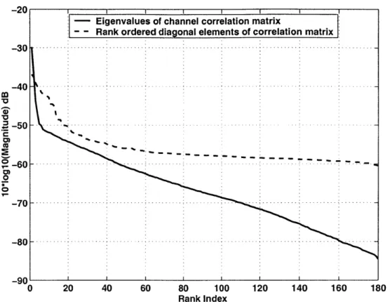
Reduced complexity methods exploit certain characteristics of the channel impulse response so that the number of parameters, i.e. the number of degrees of freedom, that need to be adapted independently is decreased. Such a reduced-complexity DFE, for use in mobile radio channels, that utilizes the sparseness of the mobile radio channel impulse response is described in [11]. Since channel impulse responses associated with a multipath structure are often sparse in nature, one in which many of the tap gains are zero or close to zero, only the nonzero tap weights are adapted independently. A threshold detector type test is used to determine whether a particular tap weight is classified as a "zero" weight or a "non-zero" weight. This technique is particularly effective when, under the WSSUS assumption [3], the different tap weights are un-correlated. The performance improvement comes from the fact that since only the non-zero weights of the unknown system are adapted, the variance is not increased for each of the other uncorrelated zero weights of the sparse system [6]. Thus, the misadjustment error due to gradient noise can be greatly reduced depending on the number of tap gains that are classified as "zero" weight. Such techniques have been very successful in mobile radio channels. The system described in [19] uses a direct adaptation equalizer and uses such a sparsing technique to determine the equalizer taps. A sparse channel response as described in [6, 19] exists when many diagonal elements of the channel impulse correlation matrix are close to zero. A generalization

of this concept is the 'low rank' channel where all diagonal elements of the channel correlation matrix have significant magnitude but many eigenvalues of the matrix are close to zero. Even though the technique of sparse equalization is quite powerful, it does not fully exploit the characteristics of the UWA channel when, unlike mobile radio channels, the tap gains in the channel impulse response are correlated. Hence, even if a particular tap gain is designated "zero" weight, performance improvement due to lowered variance of the "zero" weight is offset by the increased bias because of the correlation between the different weights.

A generalized sparsing technique that exploits this correlation between the tap gains of the channel impulse response, should be able to overcome this previously irreconcilable trade-off ,in several realistic UWA channels, between the bias and

(24)

vari--20 1 1 1 1 1 I

- Eigenvalues of channel correlation matrix

- - Rank ordered diagonal elements of correlation matrix -30 ... -40 ~-5 0 -. . . . . . . ~-60 ...- . .. ...- - - - - - - - -0 -70 - - --90 0 20 40 60 80 100 120 140 160 180 Rank index

Figure 1-3: Sparse nature of the eigenvalues and ordered diagonal elements of the channel correlation matrix

ance of misadjustment error when sparsing methods are used. The structure of the channel impulse response correlation matrix would have to be exploited in such a generalized sparsing algorithm. Figure 1-2 shows a sample channel estimate time series showing its time varying nature.

Figure 1-3 compares ordered eigenvalues of the channel impulse response correla-tion matrix with the ordered diagonal elements of the correlacorrela-tion matrix. A sliding window of size 400 was used to compute the channel estimates and the channel cor-relation matrix was computed using 12000 channel estimates. The time constant for the process corresponded to about 1600 samples which implies that the channel cor-relation matrix was estimated over a time frame of about 7.5 time constants. As seen in figure 1-3 the eigenvalues of the channel correlation matrix are much sparser than the correlated taps of the channel impulse response.

Conventional sparsing algorithms, with the implicit assumption that the different tap gains are uncorrelated, use the traditional Euclidean multidimensional bases in

(25)

identifying "zero" and "non-zero" weights by their relative position on the tapped delay line. A generalized sparsing algorithm uses the eigenvectors of the channel im-pulse response correlation matrix as the bases and identifies the "zero" and "non-zero" weights by appropriately deciding whether the corresponding bases vector belongs to the nullspace of the channel or not. Essentially, such an algorithm would have to appropriately decide the rank of the channel subspace, equal to the number of "non-zero" weights. Since these generalized weights are now uncorrelated, it is conceivable that analogous techniques that exploited this "sparse" structure would be able to achieve an improvement in performance. It is trivial to observe that the situation with uncorrelated tap gains results in the Euclidean bases as being the equivalent bases and the tap gains as being the corresponding weights. This forms the basis of the channel subspace approach, which, as a generalization to prior channel sparsing methods, attempts to exploit the correlation between the different tap weights of the time varying channel impulse response so that only the reduced rank, sparsed in a generalized sense, subspace occupied by the channel is tracked. Naturally, this im-provement in performance, analogous to previous channel sparsing methods, depends on the extent and the efficiency with which the channel can be "sparsed" in the gen-eralized sense, or have its rank reduced. A cursory examination of the ill-conditioned eigenvalue spread of the channel impulse response correlation matrix shown in Figure 1-3 makes it conceivable to believe that if properly exploited, the channel subspace ap-proach could indeed result in drastic rank reduction and a corresponding improvement in performance. Although this interpretation of tracking the reduced rank channel subspace in the context of UWA communication is unique, there is an extensive body of literature dealing with adaptive signal processing techniques using reduced rank subspace methods. An understanding of the assumptions and limitations of such methods is needed so that practical algorithms based on channel-subspace approach can be developed and analyzed.

(26)

1.3 Prior work on subspace methods

Subspace methods were originally developed as a way of reducing the mean squared error of estimators. Such methods inherently rely on shaping the rank of the sub-space of the relevant signal/parameter that is being estimated/detected. As a result, the variance of the estimator is reduced at the expense of introducing model bias and hopefully, the net result is reduced mean-squared error (MMSE). Adaptive algo-rithms that rely on subspace techniques are very powerful tools, used extensively in aspects of digital communications. One of the first applications for such techniques was proposed by Tong, Xu and Kailath [36]. Their proposal relied on oversampling, compared to the symbol rate, of the received signal. A subspace decomposition of the signal correlation matrix then separated the signal subspace and the noise subspace resulting in rapid convergence and better performance of the equalization algorithms. Different techniques were subsequently developed to help adaptively identify the di-mension of the signal subspace. Once effective discrimination of the signal and noise subspaces was achieved, the channel identification problem became analogous to a scenario where the channel was estimated within the subspace occupied by the sig-nal, while rejecting the subspace occupied by the noise. The orthogonality of the two subspaces guaranteed that channel coefficients obtained by operating on these sub-spaces were uncorrelated and independent. A reduction in error was obtained once the true dimension of the signal subspace was estimated. Concurrently, extensive research resulted in generalized algorithms for subspace based blind channel identi-fication [23, 1, 20, 9], equalization [35], data adaptive rank shaping [30], and linear prediction [1] that exploited the reduced rank nature of the signal subspace. These generalized methods are conceptually quite comparable to the types of algorithms that need to be developed to demonstrate the relevance and need for using a chan-nel subspace based approach to solve equivalent problems in UWA communications. These algorithms generally exploit the reduced dimension of the signal subspace. This reduced dimension either arises in the context of a source separation problem where the dimension of the subspace is equal to the number of sources, or in the context

(27)

of highly oversampled data. Implicitly, these techniques make the assumption that the channel itself is full rank or equivalently that the channel correlation matrix does not have eigenvalues close to or equal to zero . In the case of UWA communications, the data signal subspace is generally full rank; however, as stated earlier, the channel subspace is not necessarily full rank. Despite these subtle differences between tradi-tional signal subspace techniques, and the proposed channel subspace approach, there are striking similarities in that performance improvement in both cases is obtained by exploiting the reduced rank nature of the relevant parameter.

1.4 Thesis organization

This thesis is organized as follows. Chapter 2 introduces a theoretical framework for analyzing the tracking performance of least squares algorithms. Analytical expres-sions for the performance of the commonly used exponentially windowed and sliding windowed recursive least squares algorithms are derived. The channel subspace filter-ing (CSF) method is introduced and additional expressions are derived that explicitly indicate the improvement in performance to be expected by CSF of the least squares channel estimates. The special case of low-rank channels is examined and the per-formance of a directly constrained reduced rank least squares algorithm is analyzed using the methodology developed earlier in the chapter. The tracking performance due to CSF of the reduced rank least squares estimates is compared to and shown, analytically, to be equal to that due to CSF of conventional full rank least squares estimates. This equivalence is attributed to the ability of the CSF to exploit both the reduced dimensionality of such a low-rank channel, as well the correlation between the tracking error and the true channel impulse response.

These theoretical predictions and results from the previous chapter are corrob-orated using simulations in Chapter 3. Additionally, Chapter 3 examines the per-formance of the channel subspace post-filtering algorithm when a finite number of channel estimates, corresponding to finite number of received data samples, are used to estimate the eigenvectors of the channel subspace filter. It is shown that the

(28)

correlation between successive channel estimates affects the number of independent channel estimates available given a set of finite received data. The impact of a fi-nite number of independent channel estimates on errors in eigenvectors estimation is discussed analytically and using simulated data.

Chapter 4 details an adaptive channel subspace filtering (CSF) algorithm for use in an experimental scenario. The performance of this adaptive CSF algorithm is also examined in the context of a finite number of received data samples. It is again shown that a finite number of channel estimates affects the estimation of the eigenvectors of the process and subsequently the estimation of the CSF coefficients thereby affecting performance. This impact, of finite data samples, is demonstrated using simulated data. Additionally, the adaptive CSF (AD-CSF) algorithm is used to process ex-perimental data representing a range of channel conditions. The AD-CSF algorithm and a sub-optimal abrupt rank reduction (ARR) algorithm to be used in an experi-mental setup are described. The causal and non-causal variants of these algorithms are compared qualitatively in terms of their computational complexity requirements . These algorithms are then used to process actual experimental data and the improve-ment in performance due to CSF is presented and analyzed. The performance of the AD-CSF algorithm and ARR algorithm are compared to illustrate that, even in ex-perimental data, the improvement in performance of the AD-CSF algorithm is due to both the exploiting of the reduced rank of the channel and the Wiener post-filtering. As expected, the non-causal variant of the AD-CSF algorithm outperforms the causal variant, however the deterioration in performance due to the use of a causal algorithm is not substantial. The causal variant of the algorithm still demonstrates considerable performance improvement over the traditional RLS algorithm and is certainly more applicable in a realistic communications perspective. The significant computational ease in implementing and comparing the results of the non-causal variant make it a suitable algorithm for rapidly demonstrating the applicability of the CSF technique on additional experimental data sets.

Chapter 5 describes the theoretical framework for a channel estimate based deci-sion feedback equalizer (DFE). An analysis describing the impact of channel

(29)

estima-tion errors on the performance of such a DFE leads to a discussion of the theoretical improvements in performance expected due to a channel subspace post-filtered chan-nel estimate based DFE. This improvement in is explicitly demonstrated on simulated data. The improvement in performance obtained when used to process the same ex-perimental data used in Chapter 4 is also discussed.

Chapter 6 summarizes the contributions of this thesis and suggests possible direc-tions for future research.

(30)

(31)

Chapter 2 Tracking time-varying systems

Developing the framework and methodology that has been alluded to so far needs work on two fronts. Firstly, the basic underlying theory must be uncovered. Equally importantly, the technique must be shown to be useful for real-world examples. In this chapter, least-squares metrics of tracking performance are introduced, and the improvement in performance expected due to CSF of RLS channel estimates is demon-strated analytically. For low-rank channels, it is shown that CSF of the unconstrained RLS estimates can yield similar tracking performance as a directly constrained re-duced rank RLS algorithm to within the limits of the direct averaging assumption used to generate these analytical results. This forms the basis for the CSF paradigm for low-rank channels which suggests that the penalty incurred in conventional least-squares algorithms due to overestimation of the number of parameters to be tracked

can be eliminated by using the CSF approach.

2.1 Markov model for system identification

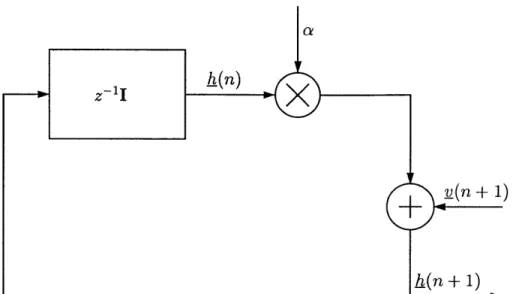
A simplified time-varying first-order Gauss-Markov model for system identification is depicted in figure 2-1. The unknown dynamic system is modeled as a transversal filter whose tap-weight vector h(n), its impulse response, evolves according to a first

(32)

(n

+)

A_(n + 1)

Figure 2-1: First-order Gauss-Markov model for time-varying system

order Markov process written in vector form as:

L(n + 1) = ah(n) + v(n + 1) (2.1)

where the underscore denotes vectors, and all vectors are N x 1 column vectors. The time-varying channel impulse response at time n is represented by the vector h(n)

with the process noise v(n) having a correlation matrix R, = E[I(n)EH(n)]. The

output of the system is given by:

y(ri) = hH(n)&~) + w(n) (2.2)

where the superscript H represents the conjugate transpose, the received data is y(n),

x(n) denotes the white transmitted data with correlation matrix Rxx = E[x(n)xH(n)] =

I, and w(n) denotes white, Gaussian additive observation noise with a variance of a.

If I a 1< 1, (2.1) and (2.2) collectively describe a time-varying system with stationary

statistics.

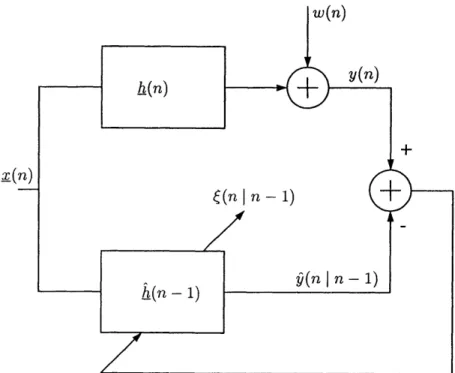
If h(n I n - 1) denotes an estimate of the true channel impulse response h(n)

(33)

w(n) h~n y (n) ( n -) - (I n - 1)

Figure 2-2: System identification using an adaptive filter

is given by:

Qn n - 1) = n I )Hn 23

The corresponding prediction error (n I n - 1) is given by: (n I n - 1) =y(n) - y(n n - 1)

=y(n) - H

In-

1)x(n)

The prediction error is used to the adapt the weights of the channel estimate h(n

I

n - 1). Throughout the remainder of this thesis, for notational simplicity, h(n - 1) is used to denote

L(n I

n - 1). The adaptation process is depicted in figure 2-2. The estimated channel impulse response L(n) is assumed to be transversal in nature too. An assumption is also made that the number of taps in the unknown system h(n) is the same as the number of taps N in the adaptive filter h(n) used to model and track the system. Although implicitly obvious, it is a very important subtlety that restricts the tracking performance of an adaptive filter, particularly when the number of taps that are tracked increases. The impact of this trade-off is discussed more formally in

(34)

later sections and the contribution of the channel subspace filtering approach shall become clearer then. It is also important to realize the assumptions made in using the above model. These assumptions, which shall be used in subsequent sections when analyzing the tracking performance of least-squares tracking algorithms, are listed below:

" The process noise vector is v(n) is independent of both the input (data) vector x(n) and the observation noise w(n).

* The input data vector x(n) and observation noise w(n) are independent of each other.

2.2 Criteria for tracking performance assessment

The channel estimation error vector, also referred to as the tracking error vector, may be defined as:

E(|n - 1) = h(n) - h(n - 1) (2.5)

As defined earlier, the prediction error is given by:

(n I n - 1) = y(n) - 9(n I n - 1)(26 _(2.6)

= y(n) - jNH(-1x)

The relationship between these two error metrics, assuming the linear channel model given in (2.2), can be written as:

H

(nI n - 1) = hH(n)x(ri) + w(n) - A n- 1)1(n)

=

(An)

- h(n - 1) H(n) + w(n) (2.7)

Substituting the expression for the channel estimation error vector given in (2.5) results in:

(35)

Based on the channel estimation error vector, f(n

I

n - 1), a commonly used figure of merit known as the mean-square channel estimation error is defined such that:

D(n) = EII A_(n) - L(n - 1) 1|2 = E[II e(n

I

n - 1) 112(

where the number of iterations n is assumed to be large enough for the adaptive filter's transient mode of operation to have finished. (2.9) may be alternately written as:

D(n) = tr[RE(n)] (2.10)

where RE,(n) is the correlation matrix of the error vector E(n | n - 1):

R,,(n) = E[(n

I

n - 1)"(n

I

n - 1)] (2.11)

The mean-square prediction error can also be expressed in terms of the mean-square channel estimation error D(n) using (2.8) such that:

E[II (n | n - 1) 112 = tr (E[f(n)EH(n)] E[j(n)j(n)_ ) +E[W2(n)]

(2.12)

= D(n) + a2

where the transmitted data vector x(n), based on the assumptions stated earlier, is assumed to be uncorrelated with the channel estimation error vector E(n). The correlation matrix of the transmitted data vector is assumed to be white so that

ReX = E[j(n),H(n)] = I, and the additive observation noise w(n) is assumed to white

with variance E[w2_(n)]

= U2 and uncorrelated with the channel impulse response

h(n). Naturally, D(n) should be small for good tracking performance. Equivalently,

given the relationship between the channel estimation error variance and the mean square prediction error in (2.12), if the statistics of the additive observation noise are stationary, then a reduction in channel estimation error leads to corresponding decrease in the prediction error. In a realistic scenario where the true channel impulse

(36)

response is unknown, it is difficult to ascertain the true channel estimation error. The mean-square prediction error can be used as a surrogate for the mean-square channel estimation error in gauging the performance of an adaptive algorithm. The notion of

improvement in performance, given this framework, is context-independent because

of the equivalence between the two error metrics, as expressed in (2.12).

The mean-square channel estimation error can be expressed as a sum of two com-ponents:

D (n) = D1(n) + 2M(n) (2.13)

where the first term D1 (n) = tr(D1 (n)) is referred to the tracking error variance and is impacted by the time-varying process. The second term D2(n) = tr(D2(n)) is re-ferred to as the observation noise induced error variance and depends on the additive observation noise. Since these terms are correlated there is no analytical way of com-puting them apriori. The terms in an analytical expression for D(n) are grouped into terms that depend on the dynamics of the process, denoted by D, (n), and terms that depend on the observation noise variance, denoted by D2(n). Separating these error terms, as above, provides insight into the tradeoff involved in designing an adaptive algorithm to track a time-varying system. For a given adaptive algorithm, best per-formance is achieved by selecting a rate of adaptation that balances the improvement due to any reduction in the tracking error variance D1 (n) with any resultant deteriora-tion due an increase in the observadeteriora-tion noise induced error variance V2(n). The term D (n) is present solely because of the time-varying nature of the system, whereas the term D2(n) is present because of the additive observation noise. If the algorithm were operating in a time-invariant environment, the tracking error variance would vanish so that the performance of the algorithm would be affected solely by the observa-tion error induced variance. While evaluating any improvement in performance due to the use of the channel-subspace filtering (CSF) approach, the channel estimation error metric shall be used for convenience even though the notion of performance im-provement is metric independent as discussed earlier. The following section formally introduces commonly used least-squares tracking algorithms, theoretically analyzes,

(37)

Received

Data Least Squares _{'Channel Estimate'}

Transmitted ,Identification h(n)

DataII

Figure 2-3: Least squares tracking algorithms

within a common framework, the tracking performance of these algorithms in terms of the channel estimation error and provides a basis for evaluating the improvement due to channel subspace post-filtering.

2.3 Least-squares tracking algorithms

Adaptive tracking algorithms generate a channel estimate A(n) based on the knowl-edge of the transmitted data, the received data and an assumed linear model for the output of the time-varying system as in (2.2). Least squares tracking algorithms, as represented in figure 2-3, attempt to compute the channel estimate so as to min-imize a cost function that is expressed as a weighted sum of the squared received signal prediction error. When ensemble averages are used to compute the channel estimate, it represents a Wiener filter solution to the minimum mean-squared error filtering problem. In a recursive implementation of the method of least squares, the estimate is initialized with assumed initial conditions and information contained in new data samples is used to update old estimates. The length of observable data to be used in making such an update is variable and depends on the specific nature of the algorithm. Accordingly, the problem of determining the channel estimate can be expressed as a least squares problem by introducing a cost function:

n S(n,

A)

= 0(n, k) 11 y(k) -hx(k) 112 k=1 (2.14) n = Z (n, k) 1| h (k) 112 k=1 where ch(k) = y(k) - hHx(k) (2.15)

(38)

is the prediction error between the received signal y(n) and the predicted signal produced using a channel estimate h. It is important to differentiate between the expressions h(n) in (2.15) and (n

I

n - 1) in (2.4). The specific contexts in which they are used should make their difference obvious. The weighting function 3(n, k) is intended to ensure that the distant past is "forgotten" in order to afford the possibility of following the variations in the observable data when the filter operates in a time-varying environment. In general, the weighting factor 0(n, k) has the property that:

0 < #(n, k) < 1, for k= 1,2,. .. ,n (2.16)

The least squares channel estimate h(n) minimizes this cost function (2.14) for a given weighting factor 0(n, k) so that:

A(n)= arg min E(n, h)

h n

= arg min E (n, k)

II

((k) 1|2 _(2.17)

k=1

=arg min #,(n, k) 11 y(k) - _hH_(k) 112

k=1

Two of the more popular least squares algorithms are the sliding window RLS (SW-RLS) and the exponentially windowed RLS (EW-(SW-RLS) algorithms. Window design, which impacts the cost function through the choice of the weighting function, is still an active area of research. Optimal window design is one of the many issues discussed in greater detail in [27]. The weighting function for the SW-RLS algorithm with a sliding window of size M is given by:

(n, k)= if k = n - M +1...In, (2.18)

(39)

while the weighting function for the EW-RLS algorithm with a forgetting factor of A is given by:

O(, k) = (1 - A)A n-k (2.19)

Solving (2.17) using the weighting functions specified in (2.18) and (2.19) results in the specific form for the SW-RLS and the EW-RLS algorithms respectively.

2.4 SW-RLS algorithm

Substituting the weighting function (2.18) in (2.17) results in the following least-squares error criterion:

h(n) = arg min

S

4 k=n-M+1 M1

hx(k) - y(k) 112

where M is the size of the sliding window. This equation can be solved deterministi-cally with the channel estimate h(n) given by:

A(n) = R (n)Rxy(n) (2.21)

where the matrices Rxx(n) and Rxy(n) are computed as:

n Rxx (n) = E :(k)j"(k) k=n-M+1 n Rxy(n) = E

5

(k)y*(k) k=n-M+1

Substituting the ensemble average for Rp1(n) in (2.21) from (A.14) results in:

E[R-(n)] = R xx M

-N -1

xx M M-N- 1 (2.22) (2.23) (2.24) (2.20)

(40)

where N is the number of taps in channel estimate vector h(n) and the transmitted data correlation matrix R., = I is assumed to be white. Substituting (2.24) and

(2.23) in (2.21) it can be shown [24] that:

E[h(n)]

Z

1 _h(k) (2.25)

k=n-M+1

Ling and Proakis used a frequency domain approach in [27] to establish the approxi-mate equivalence between the SW-RLS and the EW-RLS algorithms in regimes where the fading rate of the channel is slow compared to the symbol rate. For the model given in (2.1), the parameter a characterizes the fading rate of the channel. A regime where the fading rate is slow is one where the value of the parameter a in (2.1) is very close to 1. In such a regime, the frequency domain methodology detailed in [27] leads to the following equivalence between an EW-RLS algorithm with tracking parameter A, and an SW-RLS algorithm with a sliding window of size M when the channel estimate vector has N taps:

A=1- 2

A = 1 - _(2.26)

The following section examines the tracking performance of the EW-RLS algorithm with the tacit assumption that its equivalence with the SW-RLS algorithm as ex-pressed in (2.26) provides the basis for the use of a common framework in analyzing the tracking performance of both these RLS algorithms.

2.5 Tracking performance of EW-RLS algorithm

Substituting the weighting function (2.19) in (2.17) results in the following least-squares error criterion for the EW-RLS algorithm:

A(n) = arg min An-k 11 y(k) - h x(k) 112 (2.27)

(41)

where A is a positive constant close to, but less than 1. Although the solution to this equation, for any A, is defined by a solution to a set of normal equations similar to the ones obtained for the SW-RLS algorithm, the solution may also be expressed in a recursive form. The generalized coefficient update equation for such a least squares algorithm is given by:

L(n)

= h(n - 1) + K(n) *(n n - 1) (2.28)

where K(n) is an adaptation gain vector and (n n - 1) is the prediction error defined in (2.4). The gain vector may be computed as:

K(n) =

(

Anix(i)x( x(ri) for A E [0, 11 (2.29) Subtracting (2.1) from (2.28) and using (2.5) results in:

f(n + 1 n) = ah(n) +

v(n

+ 1) - (h(n - 1) + K(n) *(n I n - 1)) (2.30)

Substituting the expression for (n I n - 1) in (2.4) and using (2.5) to rearrange some of the terms results in:

c(n

+1

|n) = (a - 1)h(n) + (I - K(n)X(n))f(n | n - 1) (2.31) - K(n)w*(n) + v(n + 1)

(2.1) and (2.31), together, form a coupled state space system that models the dynam-ics of the unknown system as well as that of the adaptive algorithm used to update the coefficients of the channel estimation error vector. Since their dynamics are cou-pled, their behavior in steady state may be analyzed by studying the dynamics of the equivalent extended state space system in steady state. Consider the augmented vector:

g(n) = - ](2.32)

(42)

Combining (2.31) and (2.1), the extended state space system governing the evolution of g(n) may be described as : h(n + 1) aI 0 _h(n) E(n +I I n) _{((a -} _{)I I - K(n)(n)} +1(n + 1) (v(n + 1) - K(n)w*(n)

Equivalently, the system may be rewritten as:

g(n + 1) = A(n)g(n) + B(n) (2.34)

where A(n) and _B(n) are defined appropriately based on term by term comparison with (2.33). (2.34) is a stochastic difference equation in the augmented vector g(n) that has the system matrix equal to A(n). For a and A close to 1, the expected value of the system matrix is approximately equal to the identity matrix for all n. This can be readily seen by noting that:

CI 0

A(n) = ((2.35)

where E[K(n)_zx(n)] = (1 - A)I [10] so that E[I - K(n)XH(n)] = AL Thus:

aI

0

I 0

E[A ) =(2.36)

((a - 1)I AI ) I

To study the convergence behavior of such a stochastic algorithm in an average sense, the direct averaging method [21] may be invoked. According to this method, the solution of the stochastic difference equation (2.34), operating under the assumption of a, A close to 1, is close to the solution of another stochastic difference equation

(43)

whose system matrix is equal to the ensemble average:

E[A(n)] =

(

0 (2.37)

((a - 1)I AI

More specifically, the stochastic difference equation in (2.34) may be replaced with another stochastic difference equation described by:

g(n + 1) = E[A(n)]g(n) + _B(n) (2.38)

Generally, the notation in (2.38) should be different from that in the original difference equation in (2.34). However it has been chosen not to do so for the sake of convenience of presentation. The correlation matrix R, is given by:

R99 = E[g(n + I)gH(n + 1)] (2.39)

where the expectation is taken with respect to the transmitted data vector x(n) and the time-varying channel impulse response h(n). Expressing g(n + 1) as in (2.38), the steady state correlation matrix R, may be expressed as:

R₉₉= E[g(n + 1)gH(n + 1)] (2.40)

= E[A(n)]E[g(n)g(n)]E[AH(n)] + E[_B(n)B()]

where it is assumed that the process noise vector v(n), the transmitted data vector I(n), Gaussian additive observation noise w(n), and the adaptation gain vector K(n) are uncorrelated with both the channel impulse response vector _h(n) and the channel estimation error vector (n

I

n - 1). Since g(n) can be written as (2.32), the steady state correlation matrix R, can be expressed in terms of the corresponding sub matrices as:

R99 = Rhh Rh) (2.41)

(44)

where:

Rh, = E[h(n)hH(n)] (2.42)

Rhf= E[h(n)tH(n) (2.43)

Rch = E[&)hH(n)] (2.44)

RE( = E[(n)H"(n)] (2.45)

are the corresponding correlation sub-matrices. For notational convenience C(n) shall be interchangeably used with (n - 1) to represent the channel estimation error vector given in (2.5). The correlation matrix R99 of the augmented vector g(n) under steady state (when n is very large) can be written as:

H

Rhh RhE aI 0 Rhh RhE aI 0

REh REE (a - 1)1 AI REh REE (a - 1)I AI (2.46)

+ E[B(n)BH(n)]

It is assumed that the additive observation noise w(n) is zero mean and uncorrelated with both the transmitted data vector x(n) and the process noise vector i(n + 1).

Furthermore, the independence between the Gaussian additive noise w(n) and the transmitted data vector is exploited _(n) in deriving the expression:

E[K(n)w*(n)KH (n)w(n)] = E[K(n)KH (n)]E[w2 _n _(2.47)

= U.2(1 -

A2R-so that E[B(n)BH(n) in (2.46) can be written as:

E[_B(n)BH()

E & ++(n + 1) -K(n)Hw(n) (2.48)

A channel subspace post-filtering approach to adaptive equalization

A channel subspace post-filtering approach to adaptive

equalization

or

IAPR, 16

2002

I

..

. . . ..

C

. . . ..

A channel subspace post-filtering approach to adaptive

equalization

by

Rajesh Rao Nadakuditi

Abstract

Acknowledgments

Contents

List of Figures

Chapter 1

Introduction

1.1

Prior work

1.2

Receiver Design: Issues and Challenges

1.2.1

Characteristics of the UWA channel: Time-Varying

Multipath

1.2.2

Receiver Design: Current Techniques and Obstacles

1.2.3

Receiver Design: Complexity Reduction

1.3

Prior work on subspace methods

1.4

Thesis organization

Chapter 2

Tracking time-varying systems

2.1

Markov model for system identification

(n

In-

I

L(n I

2.2

Criteria for tracking performance assessment

(An)

I

I

I

I

2.3

Least-squares tracking algorithms

A)

I

II

2.4

SW-RLS algorithm

S

5

-N -1

Z

2.5

Tracking performance of EW-RLS algorithm

L(n)

(

v(n

+1

0

(

I