Simplified welding arc model by the finite element method

Publisher’s version / Version de l'éditeur:

Computers and Structures, 53, 5, pp. 1235-1241, 1994

READ THESE TERMS AND CONDITIONS CAREFULLY BEFORE USING THIS WEBSITE. https://nrc-publications.canada.ca/eng/copyright

Vous avez des questions? Nous pouvons vous aider. Pour communiquer directement avec un auteur, consultez la première page de la revue dans laquelle son article a été publié afin de trouver ses coordonnées. Si vous n’arrivez Questions? Contact the NRC Publications Archive team at

PublicationsArchive-ArchivesPublications@nrc-cnrc.gc.ca. If you wish to email the authors directly, please see the first page of the publication for their contact information.

NRC Publications Archive

Archives des publications du CNRC

This publication could be one of several versions: author’s original, accepted manuscript or the publisher’s version. / La version de cette publication peut être l’une des suivantes : la version prépublication de l’auteur, la version acceptée du manuscrit ou la version de l’éditeur.

For the publisher’s version, please access the DOI link below./ Pour consulter la version de l’éditeur, utilisez le lien DOI ci-dessous.

https://doi.org/10.1016/0045-7949(94)90171-6

Access and use of this website and the material on it are subject to the Terms and Conditions set forth at

Simplified welding arc model by the finite element method

Chidiac, S. E.; Mirza, F. A.; Wilkinson, D. S.

https://publications-cnrc.canada.ca/fra/droits

L’accès à ce site Web et l’utilisation de son contenu sont assujettis aux conditions présentées dans le site LISEZ CES CONDITIONS ATTENTIVEMENT AVANT D’UTILISER CE SITE WEB.

NRC Publications Record / Notice d'Archives des publications de CNRC:

https://nrc-publications.canada.ca/eng/view/object/?id=737ed301-f67f-4a54-bb85-03c2726ab445

https://publications-cnrc.canada.ca/fra/voir/objet/?id=737ed301-f67f-4a54-bb85-03c2726ab445

Sim plifie d w e lding a rc m ode l by t he finit e e le m e nt m e t hod

N R C C - 4 2 0 9 3

C h i d i a c , S . E . ; M i r z a , F . A . ; W i l k i n s o n , D . S .

J a n u a r y 1 9 9 4

A version of this document is published in / Une version de ce document se trouve dans:

Computers and Structures, 53, (5), pp. 1235-1241, 94, DOI:

10.1016/0045-7949(94)90171-6

http://www.nrc-cnrc.gc.ca/irc

The material in this document is covered by the provisions of the Copyright Act, by Canadian laws, policies, regulations and international agreements. Such provisions serve to identify the information source and, in specific instances, to prohibit reproduction of materials without written permission. For more information visit http://laws.justice.gc.ca/en/showtdm/cs/C-42

Les renseignements dans ce document sont protégés par la Loi sur le droit d'auteur, par les lois, les politiques et les règlements du Canada et des accords internationaux. Ces dispositions permettent d'identifier la source de l'information et, dans certains cas, d'interdire la copie de documents sans permission écrite. Pour obtenir de plus amples renseignements : http://lois.justice.gc.ca/fr/showtdm/cs/C-42

ｾｐ･ｲｧ｡ｭｯｮ＠

0045-7949(94)E0224-P

Cflmput<•Y.\" &: Strut·1urr.1· Vol. 53. No.5. pp. 1235-1241. 1994 Copyright I" 1994 Elsevier Science Ltd Printed in Great Britain 0045-7949/94 S7.00 + 0.00 c H h I K N 2 q T TA, T0 I

v

v p

r

e

A SIMPLIFIED WELDING ARC MODEL BY THE

FINITE ELEMENT METHOD

S. E. Chidiac,

t

F. A. Mirzat and D. S. Wilkinson§

tStructures Laboratory, Building M-20, Institute for Research in Construction, National Research Council Canada, Ottawa, Ontario KlA OR6, Canada

:j:Department of Civil Engineering and Engineering Mechanics, McMaster University, Hamilton, Ontario L8S 4L7, Canada

§Department of Materials Science and Engineering, McMaster University, Hamilton, Ontario L8S 4L7,

Canada

(Received 4 February 1993)

Abstract-A welding arc model is proposed to determine the thermal cycle for various materials and for different weld types. In this paper we discuss the iterative procedure employed for non-linear heat transfer analysis using the finite element method, and in particular the boundary conditions employed to determine the heat generated in the HAZ and its dissipation during welding. The model only focuses on the grain growth zone with the objective to compute the thermal regime that controls the microstructural changes that occur during welding. Both solidified weld and liquid-solid transition zones are excluded from the modeL The heat generated by the arc is applied to the vertical face of the welded edge and ;; indifferent to the size of the HAZ. The analytical results obtained for low carbon steel and for austenitic stainless steel, and for GMA and GTA weld types, correlate well with the observed experimental data reported in the literature.

NOTATION

specific heat at constant pressure (caljkg

oq

heat generated by the electric power (J/sec) coefficient of surface heat transfer (caljcm2 _sec

_oq

arc current (A)

thermal conductivity in the principal directions (caljcm sec

oq

isoparametric shape function heat input per unit volume (J/cm3₎ heat input per unit area on boundary

r

0

temperature (0 C)

specified and surrounding temperature

eq

time (sec)

arc voltage (V)

velocity of the welding arc (em/sec) density (kgjm3₎

running coordinate along the boundary

directions cosines of the unit outward nonnal to the boundary

parameter that controls the time marching scheme arc efficiency

INTRODUCTION

along the joint. However, its introduction ignites a set of complex and interrelated phenomena that are difficult to visualize. In particular the heat and mass transfer that occurs in the weld and its immediate surrounding and the micro- and macro-phenomena that affect the weld soundness, capacity and distortion, have yet to receive a co·.nprehensive and complete solution. In the past, experience had emerged as the driving force in the development of the state-of-the-art without sufficient understanding of the phenomena themselves.

Fusion welding, electrical resistance welding, solid-phase welding, and liquid-solid solid-phase joining, and adhesive bonding are the five basic categories that constitute the joining processes [I]. Fusion, and in particular arc welding, is the oldest metal joining and still the most widely used one in North America [2]. Its application ranges from fabrication of large structures (ships, bridges, etc.) to joining small ones such as thin pipelines. The process itself is nothing more than applying an intense and concentrated heat

Rosenthal [3] and Rykalin [4] who recognized the importance of accurately predicting the thermal regime, had proposed a closed form solution for a moving point source. In their solution, the thermo-physical properties and boundary conditions are assumed constant. Myers et al. [5] have since shown that simplified approaches are not adequate for the analysis of welds. To this end, numerical methods such as the finite difference method and the finite element method have emerged as the tools to assist in the solution process. However, the problem is more than just non-linear. It involves numerous phenomena such as phase changes, microstructural changes, con-vective as well as conductive heat flow and also their combined effect on the workpiece, which result in plasticity, distortion and residual stresses. More comprehensive models are being proposed now to treat not only single phenomenon but also the inter-relationship that exist between them. Several authors [6-10] to name a few, have proposed comprehensive 1235

1236 S. E. Chidiac et ai.

models to investigate in depth the temperature field, the microstructural changes and plastic deformation that occur in the heat affected zone, HAZ.

The importance of the heat source model cannot be underestimated since its application dictates the magnitude and distribution of the temperature in and around the weld. Numerical models for welding heat sources have been proposed by many researchers and their progress was reported by Goldak eta/. [11]. Since then, Tekriwal et a/. [12], Okada et a/. [8], Chidiac and Mirza [13], and Kim and Eager [14] among others have either proposed new models or modified previously reported ones in order to. satisfy experimental observations. The most accurate and widely used model for arc welds comprises a double el1iptical disk with Gaussian distribution of flux on the surface of the weld coupled with a double ellipsoidal function of power density with a Gaussian distribution to model impingement of the arc and another double ellipsoid with Gaussian distribution to model the energy distributed due to stirring of molten metals. However, the primary objective of this study was to focus on the grain growth zone of the HAZ itself rather than the molten zone. In that respect, the model previously suggested by Chidiac and Mirza [13] is adopted since preliminary -studies have indicated that its implementation generates results that are representative of collected experimental data. The model simulates a Gaussian distribution of the electric energy generated by the welding arc. Also, since the molten zone is not included in the analysis, there is no added advantage to select a complicated heat source model that takes both the effects of stirring and latent heat releases into consideration. The primary objective of this study is to develop a simplified model for welding arc. The finite element formulation used in conjunction with the heat transfer theory, the iterative procedure implemented to solve the non-linear system and equations, and the models employed in the analysis are briefly presented in this paper. The potential of the proposed model is then explored by comparing the model results to experimental data for two different metals, low carbon steel and stainless steel, and for different weld types, GMA and GTA.

HEAT BALANCE EQUATION

The calculation of the temperature field in the welded plate is based upon the transient heat con-duction and is governed by the following differential equation:

opcT = V · K(VT)

+

Q

8t (I)

The heat flow is also subject to

the

Dirichlet

bound-ary condition where the temperature is specified for

(2)

and the Cauchy boundary condition where all modes of heat transfer, namely conduction, convection and radiation are included and are represented with the following expression

The spacewise discretization of eqns (1)-(3) is accomplished with the use of isoparametric finite elements. The three-dimensional, 20-node element has been employed to model the transient heat flow [15, 16]. The unknown temperature field, T, within an element is approximated using the same

steady-state shape functions N1, employed by the element,

where

'

T=

L

N,(x,y,z)T,(t) (4)

,.1

and in which n is the number of nodes per element. The discretized equations of heat balance are then obtained by applying the method of weighted residuals combined with the Galerkin weighting procedure, and are given by

[AJ{T)

+

[Hl{T} +{F)= {0}, (5)

[A], [H] and {F) are the conductance matrix,

the capacitance matrix and the heat load vec-tor, respectively. These matrices are evaluated using Gaussian-quadrature with 27 integration points.

Linear interpolation using the two-point recurrence scheme has been implemented to obtain the solution at subsequent times. This implies that the time inte-gration operator [17J becomes dependent on a single

parameter, 8. In this study, the value of 8 = 0.667 has

been chosen since it was found to render better results for non-linear problems [18]. To control numerical instability, attention should also be focused on the size of the finite elements [19].

ITERATIVE APPROACH

To account for the non-linearities expected in the thermal properties and boundary conditions, a residual method has been implemented to minimize possible drifting in the solution during the analysis. The accumulation of the errors depends on the fluctuation in the temperature field, and to obtain a better approximation and faster convergence, an implicit approach which is embedded in the heat balance matrices is employed. The heat balance matrices become

[A]'+'= (l-8)[A]'

+

O[A]'+ I

'

'I

.,

1238 S. E. Chidiac er at. Welding arc L L=350mm b=150mm t"' 18 mm I= 170 A v :28 v v

=

2.54 mm/sc:c

Fig. 2. Geometry and mesh pattern of the specimen, and properties of the welding arc.

with the experimental data shows that the model satisfactorily predicts the peak temperature and cool-ing rates close to the fusion boundary. Figures 4 and 5 show the isothenn plots in the plane section of the plate. These figures indicate the pattern of heat flow and can be used to obtain the quasi-steady-state temperature distribution with respect to the moving arc. Also by drawing the isotherm corresponding to the HAZ boundary temperature, one can approximate its size.

Case II: 316 stainless-steel

(a) Bead-on-edge weld. The first 316 stainless-steel

specimen studies is that of a weldment using a

bead-on-edge geometry with a GMA process. It is

assumed that the heat is distributed equally between the two welded pieces and hence allows the use of symmetry. The finite element mesh for the

three-dimensional heat flow analysis is shown in Fig. 6

along with the properties of the welding arc (GMA

process). The thennophysical properties for the stainless-steel and the surface boundary conditions

that are used in the analysis are given in Table 2.

Figure 7 plots the peak temperature reached across the width (i.e. away from the weld) at the centreline obtained from the finite element analysis. In the same figure, the experimental values measured by Hwang [22] using liquid indicators and thermocouples are indicated. The results show that the model not only

- - Presetlt study - - - Experimetltal rc:sults, Kilhara el a/. [21]

'

375

---I 0 22.5 45.0 67.5 90.0 Time (sec)

Fig. 3. Thermal cycle of the heat affected zone of a

bead-welded specimen. 22 30 100 300 600 1100

Fig. 4. Evolution of temperature CCC) at t

=

23.62 sec.

22

30

so

100 300

Fig. 5. Evolution of temperature CC) at t =47.24sec.

Table I. Thennophysical properties for low carbon steel and surface heat coefficient Entity

Thermal conductivity (cal/cm sec

oq

Density, specific heat

(ca1jcm1 _"C)

Surface heat coefficient (caljcm2 _sec

_cq

Time step (sec)

T < 700'C 700'C <; T < 8JO'C T;;. 830'C Value K ｾ＠ 0.121-7.0 X IO-'T K ｾ＠ 0.1474- !.077 X IO-'T K

=

o.o25

+

4.0

x

w-

5_r Reference Argyris eta/. [23] T < 600"'C pc

=

0.88

+

7.833 X

w-

4

r

Argyris eta!. [23] 600'C.; T < 630'C pc ｾ＠ -2.85

+

7.0 x JO-'T 630'C <; T < 800'C pc ｾ＠ 3.346-2.835 x 10-'T T ｾ＠

soooc

pc = 0.79

+

3.6 x w-.lr h

=

l.757 X 10-4

₊

_1.3472

X

w-n

+

2.6106 X 10-10₇2

+

_{!.872 X}

w-

12_T1 _{Beer and Meek [20]}

90.0 one of a :3.62 sec. +7.24 sec. :nee at. [23} a/. [23} Meek [20}

A simplified welding arc mode! !239

Arc c-''

T

b

I

t

ｾ＠

L Dimensions: L = 121.92 em b = 10.16 em t = 1.27 em x = 2.54 em Weld properties: GMAweld l = 250 A V =27V v = 1.19 em/sec Eff. = 0.43 GTAweld l = 324 A

v

=12

v

v = 0.655 em/sec Elf.= 0.51

Fig. 6. Geometry and mesh pattern of the specimen, and properties of the welding arc (GMA and GTA weld).

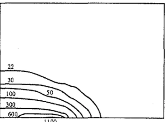
predicts the peak temperature well near the fusion zone but also has given satisfactory results away from the welded edge. Figures 8-13 display the evolution of temperature as the welding arc moves across the

plate. From these results one can observe the ｱｵ｡ｳｩｾ＠

steady-state temperature distribution. In Fig. 14, the temperature versus time of a point located 25.4 mm away from the welding edge and on the surface is plotted. Experimentally measured data are also displayed on the same figure. The model appears to produce results that represent the experimentally observed heating cycle.

(b) ｈ･｡ｴｾｯｮｾ･､ｧ･＠ weld. The second ｳｴ｡ｩｮｬ･ｳｳｾｳｴ･･ｬ＠

specimen studied is that of a weldment using a

ｨ･｡ｴｾｯｮＭ･､ｧ･＠ geometry with a GTA process. Again it is assumed that the heat is distributed equally and therefore, with the use of symmetry, only one half of the plate is analysed. The finite element mesh for the three-dimensional heat flow analysis is similar to the bead-on-edge weld as, shown in Fig. 6, as are the properties of the welding arc (GTA process). The material properties and boundary conditions employed in the analysis are given in Table 2.

The peak value of nodal temperature plots ob-tained from the finite element analysis are shown in

600,---, - - Present study A Liquid indicator (22) D Thermocouple[22]

e

200

§

ｾ＠ Ｇｯｯｬ｟Ｋ］ＺＺＺＺＺＺ［ＺｾＺ］ｊＮＺＺＺＺｊ＠

_{0 2 4 6 8 10}

Distance away from welded edge (em) Fig. 7. Peak temperature distribution (GMA weld).

20

oc

40 °C 70

oc

100

oc

200

oc

40Q°C 600°C

Fig. 8. Evolution of temperature ("C) at t

=

2.12 sec.

20

Fig. 9. Evolution of temperature ("C) at t = 23.28 sec.

Fig. 15. Experimental data measured by Hwang[22] using liquid indicator and thermocouples are plotted on the same figure. Comparison of the two results indicates that the model produces satisfactory results.

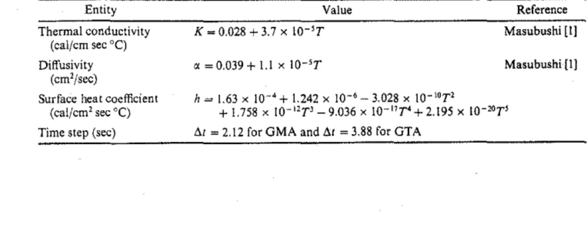
Table 2. Thermophysical properties for stainless-steel and surface heat coefficient

Entity Thermal conductivity

(caljcm sec

oq

Diffusivity (cm2_jsec)

Surface heat coefficient (cal/cm2 _{sec "C)}

Value Reference

K=0.028+3.7x 10 'T Masubushi [I]

o:

=

o.o39

+

1.1 x IO-'r Masubushi [1]

h = 1.63 x

w-

4

₊

_{1.242 x}

w-

6_{- 3.028 x}

w-

10_r2

1240 S. E. Chidiac et al.

Fig. 10. Evolution of temperature (0_{C) at t = 44.45 sec.}

40 70 100

Fig. II. Evolution of temperature ("C) at t

=

65.62 sec.

20

40 70 100

Fig, 12. Evolution of temperature (0

C) at t

=

86.78 sec.

20

40

70

Fig. 13. Evolution of temperature (0

C) at t

=

129.12 sec.

- - Present study · - - Experiment (221

20 40 60 80 100 120 140

Time (sec)

Fig. 14. Transient temperature at 25.4 mm from welding edge (GMA weld).

G

goo

ｾ＠

800

ll

_ｾ＠ 700

"

a

6oo 8 .!l 500

il

₄₀₀

ｾ＠

_e

3001- D D 8 200

"

8 1001-ﾷｾ＠

;;;

0 0 g 2 - - Present study o Liquid indicator [221 t:. Thermocouple [22}

"

4 6 8 10

Distance away from welded edge (em)

Fig. 15. Peak temperature distribution (GTA weld).

160 140 ｾ＠ ₁₂₀

!:

₁₀₀

"

ｾ＠ 80 1§

&

60

ｾ＠

t:. Present study o Experimental data [22]

....

40 20 0 40 80 120 160 200 240 280 Time (sec)

Fig. 16. Transient temperature at 25.4 mm from welding edge (GTA weld).

The transient temperature distributions at 25.4 mm away from the welding edge for both analysis and experimental data are shown in Fig. 16. Comparison of the two curves indicate that the model is capturing satisfactorily both the heating and cooling cycle.

CONCLUSION

A welding arc model employed in the three-dimensional finite element analysis has been success-fully adapted for the analysis of welded plates. Modelling of the heat source, although simple in com-parison to previously proposed models, appears to be

t40 l welding :] 10 m) weld). 22] 280 11 welding 25.4mm lysis and nparison :apturing cycle. 1e three-t success-j plates. e in

com-A simplified welding arc model 124!

adequate. It has been demonstrated that the model depicts the heating cycle observed experimentally.

Although the heat losses at the surfaces of the plate

which are difficult to quantify, the results obtained using the proposed model correlate well with the experimentally measured cooling rates. In summary, the arc model proposed in this study is adequate to determine the thermal regime in the vicinity of the weld for the purpose of computing grain growth, distortion and plastic deformations in the HAZ. How-ever, if the focus of interest is only the molten zone area, then complex models such as the one previously described are required.

Acknowledgments-The authors are grateful for the financial

support of the Natural Sciences and Engineering Research Council of Canada and to the staff of the Graphics section at IRC for assisting in preparing the figures.

REFERENCES

l, K. Masubushi, Analysis of Welded Structures. Pergamon Press, Oxford ( 1980).

2. H. B. Cary, Modern Welding Technology. Prentice-Hall,

Englewood Cliffs, NJ (1979).

3. D. Rosenthal, Theory of moving heat sources and its application to metal treatments. Trans. ASME, 68,

849-866 (1946).

4. R. R. Rykalin, Energy sources for welding. Welding in

the World 12, 227-248 (1974) [Houdrement Lecture, International Institute of Welding, London, 1974, pp.

1-23).

5. P. S. Myers, 0. A. Uyehra and G. L. Borman, Funda-mentals of heat flow in welding. Weld Res. Council

Bulletin 123, (1967).

6. D. F. Watt, L. Coon, M. J. Bibby, J. A. Goldak and C. Henwood, Modeling microstructural development in weld heat-affected zones. Acta Metal36, 69-82 (1988). 7. C. Henwood, M. J. Bibby, J. A. Goldak and D. F. Watt, Coupled transient heat transfer-microstructure weld computations. Acta Metal 36, 3037-3046 (I 988). 8. A. Okada, T. Kasugai and K. Hiraoko, Heat source

model in arc welding and evaluation of weld heat-affected zone. Trans. /S/J 28, 876-882 (1988).

9. S. E. Chidiac and F. A. Mirza. Thermal stress analysis due to welding processes by the finite element method.

Comput. Struct. 46, 407-412 (1993).

10. S. E. Chidiac, D. S. Wilkinson and F. A. Mirza, Finite element modeling of transient heat transfer and micro-structural evolution in welds: Parts II. Modeling of grain growth in austenitic stainless steels. Met. Trans. B

238, 841-845 (1992).

11. J. Goldak, M. Bibby, J. Moore, R. House and B. Patel, Computer modeling of heat flow in welds. Met. Trans.

B. 178, 587-600 ( 1986).

12. P. Tekriwal, M. Stitt and 1. Mazumder, Finite element

modelling of heat transfer for gas tungsten arc welding.

Metal Construction 19, 599R-606R (1987).

13. S. E. Chidiac and F. A. Mirza, A finite element model for thermal analysis of a metal-welding arc. Proc. of

lith Canadian Conf of Applied Mechanics, May 31-June 4, 1987, Edmonton, Alberta., Vol. 1, pp. D36-D37

(1987).

14. Y. S. Kim and T. W. Eager, Temperature distribution and energy balance in the electrode during GMAW.

Proc. of the 2nd Int. Conf on Trends in Welding Research, May 14-18, 1989, Gatlinburg, Tennessee,

pp. 13-18 (1989).

15. 0. C. Zienkiewicz, The Finite Element Method. McGraw-Hill, London (1977).

16. K. J. Bathe, Finite Element Procedures in Engineering

Analysis. Prentice-Ha!l, Englewood Cliffs, NJ (1982). 17. T. J. R. Hughes and R. L. Taylor, Unconditionally

stable algorithms for quasi-static e!asto(visco-plastic finite element analysis. Comput. Struct. 8, 169-173

(1978).

18. J. Donea, On the accuracy of finite element solutions to the transient heat-conduction equation. Int. J. Numer.

Meth. Engng 8, 103-110 (1974).

19. Z. Pammer, A mesh refinement method for transient heat conduction problems solved by finite elements. Int. J. Numer. Meth. Engng 15, 495-505 (1980).

20. G. Beer and J. L. Meek, Transient heat flow in solids.

Finite Element Methods in Engineering, The University

of New South Wales, pp. 729-740 (1974).

21. H. Kihara, H. Suzuki and H. Tamura, Researches on weldable ｨｩｧｨｾｳｴｲ･ｮｧｴｨ＠ steels. The Society of Naval

Architects of Japan (60th Anniversary Series), Tokyo

(1957).

22. J. S. Hwang, Residual stresses in weldments in high

strength steel. M.S. thesis, MIT (1976).

23. J. H. Argyris, J. Szimmat and K. J. Willam, Compu· tational aspects of welding stress analysis. Comput.