A Power Consumption Estimation Approach for Embedded Software Design using Trace Analysis

HAL Id: cea-01199765

https://hal-cea.archives-ouvertes.fr/cea-01199765

Submitted on 16 Sep 2015

HAL is a multi-disciplinary open access

archive for the deposit and dissemination of

sci-entific research documents, whether they are

pub-lished or not. The documents may come from

teaching and research institutions in France or

abroad, or from public or private research centers.

L’archive ouverte pluridisciplinaire HAL, est

destinée au dépôt et à la diffusion de documents

scientifiques de niveau recherche, publiés ou non,

émanant des établissements d’enseignement et de

recherche français ou étrangers, des laboratoires

publics ou privés.

A Power Consumption Estimation Approach for

Embedded Software Design using Trace Analysis

Yassine Ben Atitallah, Julien Mottin, Nicolas Hili, Thomas Ducroux,

Guillaume Godet-Bar

To cite this version:

Yassine Ben Atitallah, Julien Mottin, Nicolas Hili, Thomas Ducroux, Guillaume Godet-Bar. A Power

Consumption Estimation Approach for Embedded Software Design using Trace Analysis. Euromicro

Conference series on Software Engineering and Advanced Applications (SEAA), Aug 2015, Funchal,

Madeira, Portugal. �cea-01199765�

A Power Consumption Estimation Approach for

Embedded Software Design using Trace Analysis

Yassine Ben Atitallah

, Julien Mottin

, Nicolas Hili

, Thomas Ducroux

, and Guillaume Godet-Bar

1

_{CEA, LETI, MINATEC Campus, F-38054 Grenoble, France}

2

_{STMicroelectronics, Grenoble, France}

3

_{MAGILLEM Design Services S.A.S, Paris, France}

{yassine.benatitallah,julien.mottin,nicolas.hili}@cea.fr , thomas.ducroux@imag.fr, godet-bar@magillem.com

Abstract—With the explosion of advanced power control knobs such as dynamic voltage frequency scaling, mastering energy constraints in embedded systems is becoming challenging for software developers. Several power estimation techniques have been proposed over the past years, from electrical level to more abstract models such as SystemC/TLM. They offer various trade-offs between performance and accuracy, but suffer from a num-ber of shortcomings. They are expensive and time-consuming, requiring intricate models of the architecture and finally, fail to be applied from the software developer perspective. In this paper, we propose a lightweight and cost-effective approach suitable for software developers. It relies on trace analysis and high-level modeling of architectures to perform quick and efficient power consumption estimations without loosing accuracy. This approach is fully supported by a tool and is validated using a simple thermal mitigation case study and checked against physical measurements. We show that, for our case study, the relative error between our tool and real values is 8% in average.

Keywords : power consumption, embedded software design, power management and trace analysis.

I. INTRODUCTION

Estimating the power consumption of embedded applica-tions is a crucial task [1] that requires a good knowledge of not only the application itself, but also the hardware platform (HW) that executes it. Understanding the HW specific features is required to achieve the best power efficiency. Runtime power management design is however often left to the software developer who needs to master the complexity resulting from the heterogeneity of the models he or she has to interact with: programming models, toolchains, HW descriptions (datasheets) and power profiles of the execution platform.

Over the last decade, many dynamic power management components have been proposed and integrated in HW plat-forms. The most popular techniques include Power Gating [2], Dynamic Voltage Frequency Scaling (DVFS) [3] or recently CPU migration using specific HW support such as In-Kernel switcher for big.LITTLE architectures [4]. All those techniques can be used at runtime and need to be monitored precisely to limit the impact on the performance. While quantifying the performance impact can be straightforward for the software developer who knows what performance metric is relevant for his or her application, fast and precise power estimation of an entire execution can become really hard.

To manage this complexity, several approaches have been proposed [5]. They usually rely on power models at different HW abstraction layers including gate-level, Register Transfer Level (RTL), functional level and so forth, offering various accuracy / performance trade-offs. However while low-level models are accurate, they are often too complex, relying on intricate electrical descriptions and are therefore not relevant for software developers. High-level models are more easy to handle from, but are less accurate and may require additional work from software developers who possibly need to extract an application model from the original source code or execute the application on a platform model not always available.

Another possibility for the estimation of the power con-sumption from the software developer perspective would be direct physical measurement. Even if it could be feasible for systems with a quite regular power profile, it becomes harder for circuits with a high dynamic in their power consumption. For instance Internet of Thing (IoT) nodes used in [6] may op-erate in transmission mode with an electrical current of17mA, and in idle mode with a residual current of 10µA. Measuring so different currents would require to use different probes: this cannot be achieved while executing the application.

In this paper we propose a power estimation approach based on trace analysis that does not require the software developer to access more than the targeted HW and its vendor datasheet. This approach allows the HW vendor and the software developer to interact using the IP-XACT standard for all the platform documentation. We introduce a simple extension to capture power profiles of HW components based on finite state machines. This extension is authored by the vendor and come along with the datasheet, and can be seen as a formal documentation of textual information regarding power in state-of-art datasheets. The software developer can then execute its multiple application configurations on the targeted HW and produce execution traces. Thanks to the IP-XACT model, it is then possible to filter the traces to only keep the information relevant with respect to the proposed extension, to drastically limit the traces size growth. Based on the HW documentation and the filtered execution traces, a power estimation is then computed for the software developer for all the candidate application configurations to help him select the best one.

The rest of this paper is organized as follows. Section II introduces the related works. Sections III and IV detail both

IP Provider Software Developer <component> <name>. . .</name> <vendor>. . .</ vendor> <memoryMaps> <!−− . . . −−> </memoryMaps> </component> IP-Xact Description Behavior Modeling Power Annotation Trace Analysis Software Execution

Power Behavior Model

. . . w r i t i n g 4 b y t e ( s ) a t 0 x4. . . w r i t i n g 0 x00 a t 0 x400503a4 w r i t i n g 0 x01 a t 0 x400503a5 w r i t i n g 0 x00 a t 0 x400503a6 w r i t i n g 0 x02 a t 0 x400503a7 Trace A B C D rd reg.bf wr reg.bf [value=0x1] A 29% B 12% C 19% D 40%

Power Consumption Estimation

1

2 2 3

4

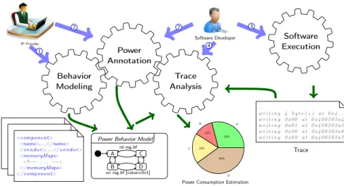
Fig. 1: Proposed Estimation Process

the proposed approach and the tool we developed to support it. Finally, section V describes the experiment we performed to estimate the power consumption on a real case study executing several power strategies and compares the results with real physical power measurements.

II. RELATEDWORK

Techniques for estimating and optimizing power consump-tion have been intensively studied over the past [5]. Many power models have been proposed at all levels of abstraction: from electrical level to functional ones [7]. While low-level models provide accurate results, they suffer from a number of shortcomings. Their application can be cumbersome, requiring specific equipments and knowledge and finally are expensive and time-consuming. Therefore, those techniques are not rel-evant for software developers who utilize high level power models.

High level power models can be classified into two main categories, Instruction Level Power Analysis (ILPA) [8] and Functional Level Power Analysis (FLPA) [9], [10]. ILPA techniques permit to estimate the consumption of a single processor, provided a detailed cost model of each instruction plus inter-instruction overheads cost models. ILPA is then conducted using an Instruction Set Simulator (ISS) that has to be delivered and integrated in a virtual platform simulator, not able to run the application code with the same performance as the real HW.

FLPA techniques abstract the HW to extract power models. These models are used either by a platform model (simulator) or by the application code (code-based analysis). Recent work by [11] aims to use UML-based diagram models to estimate the power consumption of embedded applications, with the major benefit of relying on a widely used standard for their functional power model. Work presented in [12] uses an UML profile to extend MARTE model for non-functional aspects like power consumption for embedded system development. Power consumption is modeled using state machine annotations based on prior knowledge, specifications, or measurements from prototypes. Application software is split in operation modes

that are mapped to execute on the power state machines. [13] proposes a multi-view power model approach according to knowledge and expertise based on the UML, MARTE and SysML standards. However, all those techniques require either to derive an application model from the original source code with additional efforts for the software developer, or to execute the application on a platform model that is not always available or may require additional costs once the real HW has been shipped to the software developer.

The main drawback of these techniques is to rely on abstracted HW models rather than comprehensive real HW descriptions. Such descriptions are currently address by stan-dards like IP-XACT standard [14]. IP-XACT can be seen as an electronic version of the vendor datasheet of an HW platform. It gives a formal specification of the structural information of the platform and how its constituting components are hierarchi-cally connected together. However, IP-XACT lacks of concepts to describe the functional part of the HW. The functional part is usually defined with ad-hoc code such as VHDL linked to the model, preventing to perform straightforward analyzes for power consumption estimation. On the other hand, UML behavior diagrams such as State machine diagrams are well suited to define the functional part of the system, but they lack of concepts related to the HW.

To address this issue, we present in the next section a new approach for power consumption estimation. It is based on an extension of the IP-XACT standard that captures power information and can be served as a unique, complete and comprehensive documentation for the SW developer.

III. PROPOSED ESTIMATION PROCESS

We propose in this section a lightweight approach to esti-mate the power consumption of System-on-Chip applications. It is a trace-based software approach that is involved both at design time and execution time. This approach has several advantages. It is cost-effective, time-saving, easy-to-use by non-expert users and is fully supported by a tool presented in section IV.

Fig. 2: Clock Generator Registers

behavior modeling, power annotation, software execution and trace analysis. The two first steps are performed by the platform vendor while the two others are preformed by the software developer.

The input of the approach is an Hardware Component Model, describing the structure of a System-on-Chip or part of a SoC. This model is based on the IP-XACT standard. It can be seen as a comprehensive formal documentation of a hardware platform. In particular, it gives structural information on its content (e.g., registers, signals, address map, bus width, etc.). To configure a hardware block or control its operation, software interacts with its registers. The impact of a register access by the software is part of the vendor documentation. Typically, the registers are decomposed in bitfields to allow a hardware component to hold several variables in the same register. The registers are memory mapped for the software, so that reading or writing to a specific register requires a memory read or write at specific address. This address can be computed from the IP-XACT model, using the hierarchical definition of the memory map. For our approach we only focus on the definition of the registers, their bitfields and their access modes.

Each Hardware Component Model described in IP-XACT owns a local memory map. This map includes a set of local registers. A register is defined with its offset, i.e., its initial address in the memory map, its width and its access mode. Access mode can be set to Read-Only (RO), Write-Only (WO) or Read-Write (RW). At finer grain, a register is composed of bitfields. A bitfield is also defined by an offset, i.e., its initial address in the register, an access mode and a width. Fig. 2 is an extract of a documentation about the local memory of the Clock Generator IP. The Clock Generator has four registers to configure each frequency mode and an additional register to switch between frequency modes. From this description one could derive the Clock Generator Hardware Component Model. Listing 3 illustrates an extract of IP-XACT description of the component.

A. Energy Behavior Modeling

In our approach, we introduce an extension of the the struc-tural definition of IPs by adding a model of their functional behaviors. It is done in the Behavior Model step. This model

< s p i r i t : c o m p o n e n t> < s p i r i t : n a m e>ClkGen</ s p i r i t : n a m e> < s p i r i t : b a s e A d d r e s s>0 x0</ s p i r i t : b a s e A d d r e s s> < s p i r i t : r a n g e>0x2C</ s p i r i t : r a n g e> < s p i r i t : w i d t h>32</ s p i r i t : w i d t h> < s p i r i t : r e g i s t e r> < s p i r i t : n a m e>C o n f i g c l k g e n</ s p i r i t : n a m e> < s p i r i t : a d d r e s s O f f s e t>0 x24</ s p i r i t : a d d r e s s O f f s e t> < s p i r i t : s i z e>32</ s p i r i t : s i z e> < s p i r i t : f i e l d>

< s p i r i t : n a m e>F o r c e f r e q m o d e v a l u e</ s p i r i t : n a m e> < s p i r i t : b i t O f f s e t>8</ s p i r i t : b i t O f f s e t>

< s p i r i t : b i t W i d t h>3</ s p i r i t : b i t W i d t h> < s p i r i t : a c c e s s>r e a d−w r i t e</ s p i r i t : a c c e s s> </ s p i r i t : f i e l d>

< s p i r i t : f i e l d>

< s p i r i t : n a m e>F o r c e f r e q m o d e</ s p i r i t : n a m e> < s p i r i t : b i t O f f s e t>25</ s p i r i t : b i t O f f s e t> < s p i r i t : b i t W i d t h>1</ s p i r i t : b i t W i d t h> < s p i r i t : a c c e s s>r e a d−w r i t e</ s p i r i t : a c c e s s> </ s p i r i t : f i e l d> </ s p i r i t : r e g i s t e r> </ s p i r i t : c o m p o n e n t>

Fig. 3: Fragments of the component hardware description in IP-XACT

captures any component state change operated during register accesses. A register access can be either a write or a read. It may both capture register accesses and verifications on values written and read. Verifications may concern the value written / read for the overall register or just for a bitfield of the register. The Energy Behavior Model is based on the UML State machines. Fig. 4 illustrates the Energy Behavior Model of a hardware component called Clock Generator. Four states, cor-responding to the four frequency modes of the clock generator are modeled. Transitions between each state are also modeled. Thus, it is possible to switch from one frequency mode to another one by writing the value of the target frequency mode to the Config_clk_gen register. In digital systems, dynamic power consumption is typically proportional to the frequency: knowing in which frequency mode the system is operating in function of the time will help us estimate is entire power profile of an execution.

At this point, it might be important to note that we are not interested here in modeling the whole behavior of an IP. Instead, we only focus on modeling a black-box behavior seen by the embedded Software and capturing any component state change that would have a direct impact on the power consump-tion on the IP. Attempting to model the whole behavior of an IP would be painful and inefficient.

As we only want to capture register accesses and evaluation on the values written or read, we choose to expand the semantic of the UML transitions. Only the trigger and the guard parts of the UML transition syntax is used. The transition follows the BNF expression below:

<transition> ::= ‘Rd’|‘Wr’ <register-name> [‘.’<bitfield-name>] [‘[’<guard>‘]’]

Clock Generator Behavior Model

freq mode 0

freq mode 1

freq mode 2

freq mode 3

Fig. 4: Clock Generator Energy Behavior Model

Each transition is triggered by a register access. Register access is either a read (Rd) or a write (Wr) access. <register-name> refers to the qualified name of a register of the hard-ware component model in its IP-XACT definition illustrated in Listing 3. <bitfield-name> refers to the qualified name of an optional register’s bitfield. One should notice that no transition should be triggered by a read or write event on a register or bitfield whose access mode does not match (e.g., a read event on a register in WO mode, a write event on a bitfield in RO mode).<guard> is an optional expression to evaluate the value written / read in the register or a particular bitfield of the register. Possible evaluations are equal, less, greater, less or equal, greater or equal or different. The guard is always evaluated after the event that may cause the transition trigger is dispatched. <value> is an hexadecimal value. When the bitfield is defined, the value refers to the data read from / written into the bitfield. Otherwise, it refers to the register value.

B. Power Annotation

At the end of the first step, an Energy Behavior Model has been produced. The power annotation step allows an IP provider to enrich the model with power annotations. These annotations can be used to weight each component state with an estimation of the power consumption. In addition, state transitions can also be annotated with absolute energy cost. As a result, the IP is now documented with power estimation knowledge from the vendor. This knowledge is then added to the energy behavior model that stores power information in a dedicated UML profile.

P (f ) = Pc+ α∗ f (1)

Equation 1 illustrates the power annotation of each state of the Energy Behavior Model of the Clock Generator IP. Pc

is a constant power consumption when the system is running and ready to execute a program,α is constant coefficient and f is the frequency of the system. Depending of the frequency we impose to any of the four frequency modes of the Clock

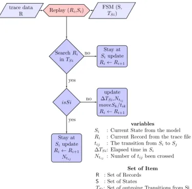
Replay (Ri,Si) trace data R FSM (S, TSi) Search Ri in TSi Stay at Siupdate Ri← Ri+1 isSi Stay at Siupdate Ri← Ri+1 Ntij update ∆TSi,Ntij moveSk/tik Ri← Ri+1 no yes no yes variables

Si : Current State from the model

Ri : Current Record from the trace file

tij : The transition from Sito Sj

∆TSi: Elapsed time in Si

Ntij : Number of tijbeen crossed

Set of Item R : Set of Records S : Set of States

TSi: Set of outgoing Transitions from Si

Fig. 5: Trace Analysis Flow Chart

Generator component, we annotate the power value of each state of the Energy Behavior Model.

C. Software Execution

The third step of our approach consists in executing the embedded software on the target platform which is a real hardware platform. We suppose that the execution can be captured in a trace file that contains all the accesses to the register of selected components, for instance the clock generator registers. This trace file also contains accurate timing results, directly captured by hardware timers. This trace file can be generated with the help of commercial tools such as Greenhills our Lauterbach, or using instrumented Hardware Abstraction Layers (HAL) with software trace generators. The trace file is a sequence of records that can be converted to the unified record format as below :

[timestamp , ( writing — reading ), value at address] D. Trace Analysis

The objective of the trace analysis step is to compute the time spent in each state and the number of time each transition has been triggered. The trace file is therefore sequentially parsed and compared to the Hardware Behavior Model. Each of its records is then analyzed, to detect if a state transition occurred. The Figure 5 illustrates the trace analysis flow chart. More precisely, the analysis operates on a Finite State Machine (FSM) and a sequence of Records (R). The FSM is a set of statesSiand a set of outgoing transitionsTSi. Each

record Rj contains a timestamp and a register access. During

the analysis, we enumerate the records and perform the two following steps. First, we search if register contained in record Rj is triggering one of the outgoing transition of current state

Using the IP-XACT model of the hardware component we can compute the absolute address of one of the component’s register and compare this address to the value contained in the record : this is done in the Resolve function. If no outgoing transition has been found, we just stay in current state and move to next record as described in Figure 5. Otherwise, we go to the second step where we simply check if the found outgoing transition has triggered a state change. If no, we only increment the corresponding transition counter. If yes, we increment the corresponding transition counter, stop theSi

timer and start the Si+1 timer. The start/stop values of the

timers are evaluated using the timsestamp information stored in record Rj.

Data:Ri,Si

Result:isM atched, isSi begin

TSi←− getOutgoingT ransitions(Si)

isM atched_{←− F alse} isSi_{←− F alse} fortj ∈ TSi do

ifResolve(tj) == Ri then

ifendState(tj) == Si then

isM atched←− T rue isSi_{←− T rue} end

else

isM atched_{←− T rue} end

end end end

Algorithm 1: SearchRi inTSi

At the end of the trace analysis step, we have collected all the data needed for the power model to estimate the overall power consumption for the corresponding software execution.

E. The Power Model

The goal of the step is to compute the energy burned by the target platform while executing a specific embedded application. The background needed for power and energy modeling for electronic circuits has been fully detailed in [15]. The power model we propose in our approach can be split in two main terms. One term for energy consumed in the states, one term for energy consumed in transitions. Energy consumption of each state EState measured in Joule can be

estimated thanks to equation 2

EState= T∗ PState (2)

WhereT is the time spent in the state, measured in second, that has been extracted thanks to the trace analysis.PState in

watt is the average power value of the state. This value has been either provided by the component vendor, or obtained by profiling. The timeT is the product of n the number of clock cycles andτ the cycle period. Is given by equation 3 as below

T = n_{∗ τ} (3)

The execution time of a transition is supposed to be constant and close to zero. We therefore have modeled the energy consumed in a transition ti as a constant value Eti.

For a given execution, the overall energy consumption of a transition triggeredN times is given by equation 4

Etransition= N∗ Eti (4)

We then assume that the total energy consumption of an executionEtotalaccording to our proposed power model is the

sum of the energy burned in the states and the energy burned in the transitions. It is given in equation 5

Etotal = K X i EStatei+ M X j Etransitionj (5)

From the equations 2 and 4, we then derive the following formula for Etotal :

Etotal= K X i Ti∗ PStatei+ M X j Nj∗ Etj (6)

At this stage of our approach, we are able to evaluate the energy consumption of a given application execution a specific target platform. The approach gives both coarse grain figures such as the overall energy consumption of the execution, and more precise metrics such as the time spent in each state, the corresponding energy burned, the number of transitions trig-gered, and a time view of instantaneous energy consumption. The approach however involves a precise sequence of oper-ations, with several actors and multiple models interactions. To efficiently support it, we offer a tool that integrates all the steps and all the models editors.

IV. TOOLSUPPORT

The presented approach is currently entirely supported by the Magillem Design Services [16] platform and Papyrus as a component of the Model Development Tools (MDT) project on Eclipse Environment. The Magillem platform helps designers to design IP components according to the IP-XACT standard. Papyrus provides a framework to extend the UML language by the use of UML profiles and customizations of UML common diagrams. The integration between IP-XACT description and UML state machine was done by extending the UML state machine through a UML profile.

The Figure 6 presents the UML profile designed called Power State Machine. A Stereotype is the profile element instantiated to customize a metaclass element from UML meta-model. The StateMachine stereotype is extended from UML state Machine and customized by adding a component property to store a link to the Hardware Component Model. The Power-State stereotype is extended from UML State and customized by adding a consumption property to store an average power value for the state. And finally, the PowerTransition stereotype is extended from UML transition and customized by adding register access event properties and a consumption property to store its energy value. With Papyrus tool, we have customized

Fig. 6: Power State Machine UML Profile

the state machine, the properties menu and the palette editors to adapt it to the Power State Machine profile. Our goal was to offer an easy-to-use tool for the different users in an embedded system development flow. Tool users are then assisted to execute the steps of our approach as described below :

• Modeling the system State Machine using a cus-tomized state machine editor and palette,

• Setting power values in the appropriate system states by a properties menu. Values are presented in W att. Setting energy cost of transitions using a similar properties menu. Values are here presented inJoule, • Loading and analyzing an execution trace. As illus-trated in section III, the software developer is respon-sible for extracting the trace. Once the trace has been produced, a dedicated replay view is featured in the tool to assist the software developer understanding and simulating its execution,

• Visualizing the detailed energy consumption report. Each state has its time elapsed and energy cost. And, Each transition has its crossed number and energy cost. As a result, the report present the total energy consumption of the application.

By extracting information contained in both the the Hard-ware Component Model and the Hardware Behavior Model, the tool assist the developer to edit the transitions in the state machine editor. The state machine model of a component is connected to its IP-XACT hardware description. While editing the transitions, an assistant is provided to the user. This assistant automatically lists available registers and bitfields, consistently with the Hardware Component Model, and checks for access modes. This prevents for instance the user to define transition guards that would imply a write on a read-only register.

V. EXPERIMENTAL RESULTS

In this section, we applied our approach to a case study involving a real hardware platform, a regular matrix multiply application, and several runtime power management strategies and demonstrate the validity of the approach and qualify its precision. First, we present a case study application. Second we conduct a power profiling step since no vendor information were available for the power characterization of our platform,

this allows us to build the power state model. Then, to validate the estimation results provided by our tool, we compare our estimations to real physical measurements. And finally, we discuss the experimental results in order to present how our approach can help the software developer to decide which power management strategy to use.

A. Case study Algorithm

The Algorithm 2 is a simple thermal mitigation strategy. Its main objective is to limit the temperature elevation of the chip while reducing power consumption and achieving maximum performance. It is based on frequency modes switch. A initial frequency mode is set at the beginning program. While the temperature remains low, the algorithm switch from the current frequency to a higher one to increase performance. If the temperature exceeds a maximum threshold, it switches to a lower frequency mode to reduce temperature. In our case study, the software developer does not know how many modes he should use, and which ones. A simple view of the algorithm is illustrated below :

Data:numberof M ode,value0,value1,value2,value3, thresholdtemp

setF requencyF orM ode(0, value0); setF requencyF orM ode(1, value1); setF requencyF orM ode(2, value2); setF requencyF orM ode(3, value3); currentM ode←− 0 ;

m we used is a real har while acquisition do temperature←− gettemperature() ; iftemperature < thresholdtemp then

ifcurrentM ode < numberof M ode then currentM ode + +;

setF requency(currentM ode); end

else

ifcurrentM ode > 0 then currentM ode− −;

setF requency(currentM ode); end

end

Algorithm 2: Case study Algorithm

We used an execution platform called STHORM [17]. It is a power efficient manycore architecture consisting of a host processor and a manycore fabric. The host processor is a dual-core ARM cortex A9 and the fabric comprises 64 computing elements. The clock of the fabric is supplied by the Clock Generator described in Figure 4. Depending on the frequencies configured for each mode, the average power values of each state of the fabric has to be defined.

B. Behavior and power modeling of the System

We consider that each frequency mode is a power state that has to be characterized with a single power consumption value. According to Power annotation process described in section III, the software developer can obtain the power cost of frequency mode from equation 1. In our case study, we have been able to identify the corresponding parameters values. Pc the constant power is 196mW and the coefficient α is

P (f ) = 196 + 0.8∗ f (7) Applying equation 7 for the four frequency modes used in our case study algorithm, we obtain the power values showed in Table I.

TABLE I: Power of frequency mode

Frequency Mode (MHz) Average Power (mW)

10 204

100 276

200 356

400 516

Depending on the frequency modes of the algorithm, the software developer updates the power value into power state property in the system behavior model.

C. Results and benefits

Table II shows three different configurations for the thermal mitigation strategy used in our case study. Depending on the strategy, 4 or 2 frequency modes are used, with various frequency values. The first strategyS1 has 4 frequency modes

(inM hz) respectively (m1= 10, m2= 100, m3= 200, m4=

400). The second strategyS2 has 2 modes (m1= 100, m2=

200) and the thirdS3 has 2 modes (m1 = 100, m2 = 400).

For all the three strategies, the execution duration T is the sameT = 25s. The last column of the table shows the overall energy cost of the strategies.

TABLE II: Energy consumption results

Application mode 0 mode 1 mode 2 mode 3 Energy (J)

S1 10 100 200 400 8.93

S2 100 200 N/A N/A 9.21

S3 100 400 N/A N/A 11.63

In order to help the software developer pick the best strategy, the energy cost has to be compared simultaneously with the application performance. For this matter, a relevant metric is to divide the number of processed items by the energy, which is equivalent to the throughput/power ratio. Traditionally efficiency is expressed in GFlop/s/W or GFlop/J where GFlop stands for Giga floating point operations. Here we don’t have precise estimation of the number of GFlop spent in our application, so we expressed the achieved efficiency in number of iterations per Joule and normalized it to 1 for the first strategy in Table III.

TABLE III: Energy efficiency comparison

Application Max Frequency Energy Normalized Efficiency

S1 400 8.93 1

S2 200 9.21 0.96

S3 400 11.63 1.19

As we can see on previous table, the strategyS3with only

2 modes at 200 and 400 M Hz is achieving the maximum efficiency. It is therefore the best choice for the software developer.

In Table IV an overview of the performance of the trace analysis in our tool is presented. The performance was esti-mated on a regular desktop computer with an Intel Core i3

processor. The two first lines respectively presents the trace size and the analysis time for the strategiesS3andS1. The last

line is a generated scenario that corresponds to an execution time of 5 minutes. In all cases, the analysis time is negligible compared to the execution time.

TABLE IV: Time consumed by the trace analysis

Data (B) Matched records Proc. time (ms) Time/record (ms)

11860 8 172.5 21.5

38790 26 193.5 7.5

458995 250 1376 5.5

D. Comparison with real measurements

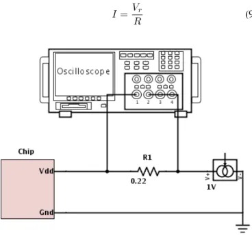
The capability of our approach has been demonstrated, we now have to estimate its accuracy. To do so, we have built an experimental set up where, it was possible to simultaneously execute the application and produce the execution trace, while capturing the instantaneous power consumption using an exter-nal tool, in our case an oscilloscope. The corresponding set-up is described in the electric schematic illustrated in Figure 7. To estimate the power of the circuit, simultaneous acquisition of its supply voltage and current has been made.

The power P is given by equation 8.

P = I∗ Vdd (8)

Vdd is the supply voltage andI is the average current. We

can get I as the ratio between the resistance voltage Vr and

the resistance valueR as illustrated in equation 9.

I = Vr

R (9)

Fig. 7: Electrical schema for power acquisition

For current measurement, a resistance has been put on the power line of the chip. This resistance was sufficiently small to avoid large voltage drops in the chip, and sufficiently large to get enough signal for the measurement. In our setup, we found thatR = 0.22Ω was a good trade-off.

Applying Kirchhoffs voltage law, we obtainVr illustrated

in equation 10 as the difference between the source voltageVs

and the chip voltage Vc.

Vr= Vs− Vc (10)

Referring to equations 8, 9 and 10, we obtain the powerP :

P = Vc∗

Vs− Vc

R (11)

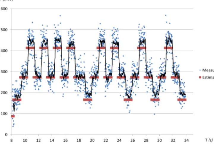
The Figure 8 shows a view of the power (in mW) variation in function of time in s for the first strategyS1. The blue dots

are the actual physical measurements of the oscilloscope. To reduce the noise, we applied a smoothing filter on the results using a simple moving average over 8 values and produced the black curve. The red plot shows the power estimation by our approach.

Fig. 8: Comparing between real and estimation power consumption measurements

We can see a really good correlation of the two curves, and computed an average relative error of 8% for our approach compared to physical measurements, which is the same error rate as reference power simulators for our platform [18].

VI. CONCLUSION

A power consumption estimation approach for embedded software design using trace analysis has been presented. This approach is well suited for software designers who have to deal with time-to-market constraints and short development cycles, who often fail to access to complex power simulators involving virtual platforms and long execution times. Here, their power management design exploration is fully supported by the tool we have developed and the power analysis is done off-line almost instantaneously. The approach we propose has also been checked against real power measurement and demonstrated to achieve state-of-art precision compared to traditional power virtual simulations. Finally, the approach is built upon industry standards such as IP-XACT and UML and leverages documentation efforts accomplished on vendor side.

Future work would be to integrate this approach in au-tomated power exploration flows, possibly for strongly con-strained domains such as IoT applications involving several platforms and distributed applications.

ACKNOWLEDGMENT

The authors would like to thank the ACOSE project for their support. It has been funded by France in the frame of a program called ”Investissements d’Avenir D´eveloppement de l’Economie Num´erique - Briques g´en´eriques du logiciel embarqu´e”.

REFERENCES

[1] C. Ebert and C. Jones, “Embedded software: Facts, figures, and future,”

Computer, 2009.

[2] D. Brooks, P. Bose, S. Schuster, H. Jacobson, P. Kudva, A.

Buyukto-sunoglu, J.-D. Wellman, V. Zyuban, M. Gupta, and P. Cook, “Power-aware microarchitecture: design and modeling challenges for next-generation microprocessors,” Micro, IEEE, 2000.

[3] M. Pedram, “Power optimization and management in embedded

sys-tems,” in ASP-DAC, 2001.

[4] K. Yu, D. Han, C. Youn, S. Hwang, and J. Lee, “Power-aware task

scheduling for big.little mobile processor,” in ISOCC, Nov 2013.

[5] S. Reda and A. N. Nowroz, “Power modeling and characterization of

computing devices: A survey,” Found. Trends Electron. Des. Autom., 2012.

[6] M. Sichitiu, “Cross-layer scheduling for power efficiency in wireless

sensor networks,” in INFOCOM, 2004.

[7] A. Bogliolo and L. Benini, “Node sampling: a robust rtl power modeling

approach,” in ICCAD, 1998.

[8] V. Tiwari, S. Malik, A. Wolfe, and M. T. chien Lee, “Instruction level

power analysis and optimization of software,” Journal of VLSI Signal Processing, 1996.

[9] J. Laurent, N. Julien, E. Senn, and E. Martin, “Functional level power

analysis: An efficient approach for modeling the power consumption of complex processors,” in DATE, 2004.

[10] H. Blume, D. Becker, L. Rotenberg, M. Botteck, J. Brakensiek, and

T. G. Noll, “Hybrid functional- and instruction-level power modeling for embedded and heterogeneous processor architectures,” J. Syst. Archit., 2007.

[11] D.-H. Kim, J.-P. Kim, and J.-E. Hong, “A power consumption

anal-ysis technique using uml-based design models in embedded software development,” in SOFSEM’11, 2011.

[12] T. Arpinen, E. Salminen, T. D. Hmlinen, and M. Hnnikinen,

“{MARTE} profile extension for modeling dynamic power management

of embedded systems,” Journal of Systems Architecture, 2012.

[13] C. Gomez, J. DeAntoni, and F. Mallet, “Multi-view power modeling

based on uml, marte and sysml,” 2012.

[14] “IEEE Standard for IP-XACT, Standard Structure for Packaging,

In-tegrating, and Reusing IP within Tools Flows,” IEEE Std 1685-2009, 2010.

[15] L. Scheffer, L. Lavagno, and G. Martin, EDA for IC System Design,

Verification, and Testing (Electronic Design Automation for Integrated Circuits Handbook). 2006.

[16] “Magillem Design Services.” http://www.magillem.com/.

[17] D. Melpignano et al., “Platform 2012, a many-core computing

accel-erator for embedded socs: Performance evaluation of visual analytics applications,” in DAC, 2012.

[18] T. Ducroux, G. Haugou, V. Risson, and P. Vivet, “Fast and accurate

power annotated simulation: Application to a many-core architecture,” in PATMOS, 2013.