Data-driven logistic planning

(1)

Data-Driven Logistics Planning

by

Christopher Aaron Richard

B.S., Electrical Engineering, United States Military Academy, 1989

Submitted to the Sloan School of Management and the Department of Electrical Engineering in Partial Fulfillment of the Requirements for the Degrees of

Master of Science in Management and

Master of Science in Electrical Engineering at the

Massachusetts Institute of Technology May, 1996

Signature of Author

Denartment of Electrical Engineering and Computer Science

Certified by

j

.onaI n.

-.

CoIsemeiIU

Senior Lecturer, Sloan School of Management .. Advisor

Certified by _ ..

Alvin W. Drake :ience and Engineering Thesis Advisor

Accepted by

Jeffery A. Barks

Associate Dezm• aOmTn-,--- J .. D -•-'r's 7 Programs

Accepted by

... forgenthaler

" ChAiT _an,Con -e on Graduate Students

OFJUL

1TECH6OLOG1996

_Eng.

JUL 1 61996

Eg

(2)

(3)

Data-Driven Logistics Planning by

Christopher Aaron Richard

B.S., Electrical Engineering, United States Military Academy, 1989

Submitted to the Sloan School of Management and the Department of Electrical Engineering in Partial Fulfillment of the Requirements for the Degrees of

Master of Science in Management and

Master of Science in Electrical Engineering

ABSTRACT

Rapidly growing, high-technology industries face especially difficult challenges in the realm of logistics management. Short product life cycles and capricious markets create conditions of great uncertainty in both supply and demand. Material planners manage inventory in an attempt to maintain a fine point of balance between satisfying customer demand and controlling

inventory levels. There are costs associated with failing to fill orders within the customers' desired lead time as well as with procuring and holding inventory. Material planners spend their days attempting to minimize these costs. The inventory system which they try to manage is one that is characterized by complex and non-linear cause and effect relationships. Human beings have difficulty understanding the effects of non-linearities, feedback and cause and effect relationships that are separated in space and time. Planners function in this confusing

environment having developed their intuition over many years. They often make decisions based on what they term "gut feel", "hard to quantify" and "soft" data.

This thesis is based on the premise that the proper and consistent use of available data in logistics planning can lead to a better balance between customer satisfaction levels and quantity of

inventory held in stock.

I present a model of the total cost of the inventory system. I present a framework that allows planners to input various pieces of relevant decision making data. The model is used to analyze

current operating procedures and recommend improvements.

Thesis Advisors:

Professor Alvin W. Drake

Senior Lecturer Donald B. Rosenfield

(4)

(5)

Acknowledgments

I would like to thank the following people for the support and advice they provided me during the course of my internship. At PictureTel Corporation: Alan Frazer, Kurt Edmunds,

Linda Quinn, Alex Nahatis, Dave McQueen, Ed Wade, Jim O'Bray, Sally Blount, Tony Rosati, Joe Sheeler, Emil Manfra, Joyce Lachance, Rick Zaccardo, Steve Szot, Jean Bortz, Mike Halligan, Michelle Mapstone, Joel Brenner, Gary Kleppe, Matt MacDonald, and Scott Fitzgerald.

I would like to extend my special thanks to Fred Bowers and Ian Bell, of PictureTel, and Al Drake and Don Rosenfield, my thesis advisors at MIT, who provided specific support for, advise regarding and endorsement of my activities.

I would like to acknowledge the support and resources made available to me during the course of my internship by the Leaders for Manufacturing Program.

(10)

(11)

Chapter 1: Introduction and Overview

Preface

Management is in transition from an art, based only on experience, to a profession, based on an underlying structure of principles and science.

Any worthwhile human endeavor emerges first as an art. We succeed before we .understand why. The practice of medicine or of engineering began as an empirical art representing only the expertise of judgment based on experience. The development of the underlying sciences was motivated by the need to understand better the foundation on which the art rested.

Without an underlying science, advancement of an art eventually reaches a plateau. Management has reached such a plateau. If progress is to continue, an applied science must arise as a foundation to support further development of the art. Such a base of applied science would permit experiences to be translated into a common frame of reference from which they could be transferred from the past to the present or from one location to another, to be effectively applied in new

situations by other managers.

-- Jay Forrester, Industrial Dynamics

The purpose of my thesis is to further the advancement of the science of management by contributing to the understanding of how we can translate art into science. One tool for

managing this translation is explicit modeling. Explicitly modeling the actual situation forces us to understand and evaluate our current policies. Explicitly modeling the desired situation forces us to form a clear picture of the paradigm which we strive to achieve'. The comparison of these two models reveals the differences and helps us create a plan to reconcile them.

Page 11

(12)

In the world of a rapidly growing, high technology company, where everyone is running as fast as they can just to keep up, and where the money is rolling in hand over fist, it is easy to overlook the need for careful analysis of current practices. While technology and first mover advantage may give a high tech company a comfortable position for some time, analysis, evaluation and improvement of business practices are necessary to survive over the long run.

Problem Statement

PictureTel Corporation has stated that making supply chain management a core competency is a fundamental component of its strategy. Currently, PictureTel has no adequate methodology to evaluate the costs associated with the policies that control the operation of its supply chain. If PictureTel is.to gain advantage by effective supply chain management, the company must have better methods for evaluating supply chain costs, particularly those costs associated with the company's own policies.

Background

PictureTel is a young, technology-based company that is experiencing rapid growth. Since 1990 the company's revenue has grown at an average annual rate of 68%. As sales have expanded, both in quantity and in geographical spread, the logistics system has been strained in an attempt to keep pace.

Over the years, policies have evolved for managing pieces of the supply chain. From time to time decisions have been made to incrementally expand its capacity and its capabilities. Though these decisions were locally logical and rational, they were not necessarily globally optimal. In fact it would be extremely difficult to determine which decisions would be best for the overall system, as there exists no measurement system that can adequately quantify the costs and benefits of such decisions.

(13)

In the summer of 1995 PictureTel reviewed its supply chain operations. An analysis by the author of the existing European distribution operation revealed that significant cost reductions could be realized by improving the inventory management and replenishment policies. This project revealed the need for an analysis of the entire supply chain system and the need for a tool that can be used to assist in inventory management. The decisions facing the company are:

* In what locations should inventory be stored?

* In each of these locations, how much inventory should be stored? * How does each inventory storage location reorder goods?

* In what shipment sizes are orders for goods satisfied?

In this thesis I address the latter three questions.

PictureTel is moving towards a business model in which it does not perform any of its own manufacturing. The company will purchase subassemblies from various vendors which will then need to be packaged and shipped to customers. In this sense, the company is mainly concerned with the integration and distribution of finished goods (of some form). However, since the lead times on some of its custom products currently exceed seven months, the slow response of the supply side of the chain must be carefully considered when planning finished goods inventory levels. The supply chain, as defined here, consists of both the incoming supply and outgoing

distribution chains.

As the company moves toward this new business model, the supply chain needs to change to support it. The current practice of routing all goods through PictureTel's warehouse in Peabody, MA is not necessarily the best practice, as the value added by this step will be questionable in the future.

(14)

Company Background

PictureTel Corporation is the market and technology leader in the videoconferencing industry. The company has three categories of products. These are room or group systems, personal or desktop systems and network systems. Each of these product types is administered by a corresponding business division. The Room Systems Division (RSD), the Personal Systems Division (PSD) and the Network Systems Division (NSD). PictureTel is attempting to capture almost all of the identified market segments with the products from these divisions.

PictureTel's technology allows videoconferencing to be conducted over switched digital telephone lines. These lines are available in most locations in the world today, though the particular type of hardware interface may vary from place to place. The heart of the technology is a proprietary video compression algorithm. This algorithm allows video signals on the order of megabits per second to be compressed, with minimal loss of picture quality, to signals on the order of hundreds of kilobits per second.

The company structure is moving towards what they term a "leveraged" model. In this business model the manufacturing and distribution of products is outsourced. PictureTel will continue to design and market their products, but most of their operational activities will occur outside of the corporation's boundaries, with direction being provided from within. Manufacturing is included in this set of outsourced activities. Currently, PictureTel's personal and network systems are manufactured entirely by third parties. Some of the room system products undergo final assembly and test procedures at PictureTel, but all of the components and subassemblies are manufactured by third parties. In the future even these systems will be completely outsourced.

In support of this leveraged model, PictureTel operations has stated that its two core competencies will be product life cycle management and supply chain management.

(15)

The Videoconferencing Industry

The videoconferencing industry is growing rapidly. The short product life cycles are on the order of 18 months. These factors combine to create a business environment that is challenging to manage.

Since 1990 PictureTel's revenue has been increasing at an average2 annual rate of 68%. This trend is graphically portrayed in Chart 1, below.

Revenue ~$O3.U $300.0 $250.0 $200.0 $150.0 $100.0 $50.0 $-1988 Annual Revenue 1989 1990 1991 1992 1993 1994 Chart 1 -Year 19 95

PictureTel Revenue Trend

There is an obvious seasonal pattern and trend exhibited in sales in this industry. There is a notable seasonal pattern within the quarter and a trend within the year. The first month of the quarter represents approximately 17% of the total quarterly sales, the second month of the quarter represents approximately 24% of the total quarterly sales and the third month of the quarter represents approximately 59% of the total quarterly sales. The first quarter of the year represents approximately 20% of the total yearly sales, the second quarter of the year represents

approximately 24% of the total yearly sales, the third quarter of the year represents

(16)

approximately 27% of the total approximately 29% of the total graphically in Chart 2, below.

%YearIy~ % Yearly 16% 14% 12% 10% 8% 6% 4% 1 2% 0%

yearly sales and the fourth quarter of the year represents yearly sales. The seasonal pattern and trend are represented

Sales

.ilii

ii

_,

13

Chart 2 -Historical Monthly Sales as a Percentage of Yearly Sales

Systems and Control: Engineering and Business

A business is a complex system designed by man. Like any other system designed by man, a business exists for a specific purpose. This purpose is to make money for its stakeholders.

When man designs an engineering system, he includes control mechanisms. These mechanisms exist in order to keep the system performing correctly, that is, to keep the system producing the desired output. Without such mechanisms the system will almost definitely go out of control and stop producing the desired output (for which it was created). So without reliable control

mechanisms, the system is not of much use.

2 Geometric average.

(17)

In an engineering system, a simple controller compares the actual output of the system to the desired output. If a discrepancy exists, it then adjusts the inputs and/or the process to bring the actual output in line with the desired output3. Such a controller is shown below, in Figure 1.

Inputs

Desired

Output Respt

Output

Figure 1 -Engineering Control System

Of course, appropriate control action requires that the controller's designer know enough about the cause and effect relationships between the system output and its inputs and processes to take the correct actions at the correct times. Indeed, most engineering systems that we encounter in our daily lives are understood well enough to make this happen under quite a variety of

conditions. If they were not, we would certainly give much more thought before boarding an airplane or stepping onto an elevator.

Like engineering systems, businesses have control mechanisms. Like engineering systems, these control mechanisms exist in order to bring each output of the system in line with the desired output. The big difference between engineering systems and business systems is the degree of understanding that the respective controller designers have about the cause and effect

relationships in the system. While these relationships are often understood quite well in engineering systems, they are frequently not at all well understood in business systems.

SDorf, 1987 4

"An Informal Note on Knowledge and How to Manage It", 1986

(18)

This lack of understanding makes it hard to design business control systems that cause the system to respond to the wishes of the designer. In fact, many times in business we encounter de facto control systems that were never explicitly designed into the system. They have come into existence because of a local need and do not necessarily act in the best interests of the broader system. Indeed, a business is so complex and the conditions in which it operates so uncertain that the concept of designing a fully integrated, holistic centralized control system to optimize the performance of a business is pretty unlikely. However, control systems do not need to be

centralized to be effective. In fact, in complex systems, an attempt at centralized control will almost never work. The attempt to centrally control the economy of the former Soviet Union is a good example of such a failure5.

While it is extremely difficult to make complex systems function properly with centralized control, it is very possible to make them function well with distributed control. Simple, local controllers can often function well to accomplish specific outcomes under diverse circumstances. Similar simple, local control mechanisms at the next level in the hierarchy can control how two lower level parts of the system interact. This model of control has been repeatedly proven in complex engineering systems ranging from technically mature chemical refineries and experimental mobile robots.

So how do we take these lessons from engineering and transfer them to business? One way is to examine the procedure that a control engineer might use to for an engineering system and use an equivalent procedure for business. Certainly such a procedure would, in the very least, provide the manager a tool for the systematic evaluation of the business system.

(19)

Procedure for Designing a Controller

During the course of my internship at PictureTel, I, from time to time, found business systems that did not appear to be functioning as intended. As a tool to aid in the systematic evaluation of a business control system, I developed the following procedure. This procedure, which was developed from my own experience in designing engineering and business control systems, provides a logical and thorough template for evaluating business control systems.

Controller Design Procedure

6

1. Identify the outputs in which you are interested. 2. Identify the desired values of these outputs.

3. Identify ways to measure the actual values of these outputs. 4. Identify the inputs and process variables that affect the outputs.

5. Identify ways to measure the actual values of these inputs and process variables

6. State your understanding of the cause and effect relationships between the inputs, process variables and the outputs.

7. Create a controller7 that, in response to a discrepancy between the desired and actual system output, causes a change in the appropriate inputs or process variables such that the

discrepancy will go away.

8. Connect the controller to a source of power, its inputs and actuators.

9. Calibrate the sensors (of the outputs, inputs and process variables) to ensure that the signals they are generating are correct.

10. Test the control system in its environment and make adjustments as necessary.

At first glance the reader may suppose that a big challenge to implementing such a procedure in a business environment is understanding of the cause and effect relationships between the inputs,

6 They key terms used in this procedure are diagrammed in Figure 1.

7 _{A controller in the engineering context is a mechanical, electrical or logical device. In the business context, it can}

take many forms. It can be a person, perhaps one who is following a procedure. It can be a system of people and

(20)

process variables and the outputs as this will determine the effectiveness of the controller. Trying to put this mental puzzle together can be overwhelming. And at this point many people would say that this task is too daunting, that these relationships can not be understood to a sufficient degree. However, I propose that, in some situations, major benefits may be realized without such a thorough understanding. In other situations, this understanding of cause and effect already does exist, and the reason that the system does not behave as desired is that one of the other conditions necessary to achieve proper controller action has not been met.

For example, the lack of business reporting tools in a business system is equivalent to not having inputs to the controller in an engineering system. Having business reporting tools of mediocre quality is equivalent to having the wrong or uncalibrated inputs. We would not expect an engineering control system to work with wrong, uncalibrated, or lack of inputs. Why should we expect a business control system to work under these conditions?

The factor that contributes the most to making control in business difficult is uncertainty. Uncertainty is ubiquitous in the business environment. Uncertainty is present in forecasts, in supplier reliability and in the performance of every humanly executed action in the system.

We do not have to accept a given level of uncertainty as inevitable. In the spirit of continuous improvement we should strive to qualify, quantify and reduce the causes of uncertainty. But while we continue to work to reduce uncertainty, we must deal with its current level wisely. This is accomplished by the proper use of techniques from the fields of probability and statistics.

Chapter Conclusions

It is the formal process of transforming the art of management into the science of management that enables a company to learn as an organization. A powerful tool that can be used in this process is modeling. While PictureTel is not currently undertaking such long term business

procedures working, whether they realize it or not, in related areas. It can be a computer program. Or it can be some combination of all of these.

(21)

improvement efforts, such efforts must be commissioned at some point if the company is to sustain its market position against such manufacturing powerhouses as Intel and Hitachi.

A business should be thought of as a system. It requires controls to function properly.

Translating engineering controller design process knowledge into the realm of business provides a powerful framework to help model and design the business.

Overview of the Remaining Chapters

In the remaining chapters I shall examine PictureTel's logistics system using the concepts discussed above.

In chapter two I describe the logistics system as it exists today.

In chapter three I present the complex inventory management problem, reduce it to a simpler form and develop an inventory cost model which can be used to help in decision making given the available information.

In chapter four I analyze the current logistics system using the controller design procedure as a logical analysis framework and the inventory cost model as a tool for evaluating inventory decisions. In this chapter I focus on the main inventory drivers: the forecast procedure and inventory control mechanisms.

In chapter five I make further analyses to include secondary inventory drivers and other aspects of the logistics system.

In chapter six I present conclusions and recommendations.

(22)

(23)

Chapter 2: The Existing State of the Supply Chain

Introduction

In this chapter I briefly describe the supply chain as it exists today. I cover the material flow as well as the information flow throughout this system.

Definition of Terms

Supply'Chain: This term refers to the route that goods follow from PictureTel's suppliers to its customers. It includes the physical locations at which goods are stored, the transportation streams that connect those locations and the business processes which cause the movement of goods throughout this system.

Material Flow

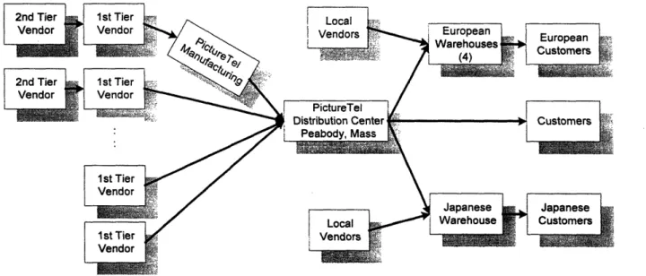
The flow of materials through the supply chain is as represented in Figure 2, below.

Figure 2 -PictureTel's Material Flow

(24)

First Tier Vendors

PictureTel has over a thousand8 vendors which directly supply goods to them. Most of these vendors are located in the United States. A large number of these vendors are located within

several hours of the Peabody, Massachusetts Distribution Center (DC), though some key vendors are quite far removed (California, North Carolina, Idaho, Wisconsin, Japan). With the exception of some of the local vendors, PictureTel pays the freight for these shipments. Lead times for products vary from days to months.

Second Tier Vendors

First tier vendors purchase materials from second tier vendors. Though functional relationships primarily exist between the first and second tier vendors, in some cases PictureTel becomes involved with the second tier vendors. This involvement is primarily through engineering as they design products and work out specifications. PictureTel is also concerned with the lead times between these first and second tier vendors as they are frequently a major component of the total product lead time.

PictureTel Distribution Center

PictureTel has one distribution center located in Peabody, Massachusetts. The vast majority of

goods that eventually arrive at the customer site flow through this location. Goods are received, stored until needed and the picked, packed and shipped.

Manufacturing

PictureTel performs a limited amount of manufacturing. This manufacturing process consists of final assembly and test on their room system products. Materials that undergo these processes are received by the manufacturing facility in Peabody, Massachusetts and then shipped, via PictureTel's truck, to the distribution center, which is less than one mile away.

(25)

Warehouses

There are finished goods warehouses located in Europe and Japan. The European warehouses are located in the U.K., Germany, Switzerland and Sweden. These are public warehouses in which PictureTel rents space as needed. These warehousing companies also coordinate delivery of the product to the customers. The vast majority of the materials that flow through these warehouses are received from the Peabody DC. Some items are purchased from local vendors though, and received at these warehouses in preparation for shipment to the customers.

Local Vendors

Local vendors supply a small number of items that can be procured locally and are geographically specific. There are about a half dozen of these local vendors per region.

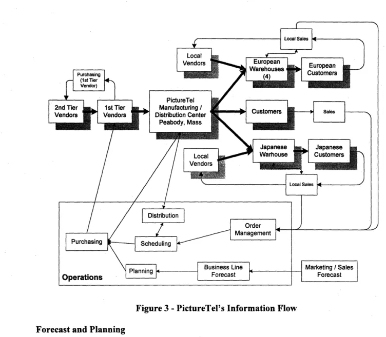
Information Flow

The information flows that control the movement of materials throughout the supply chain are presented in Figure 3. For diagrammatic simplicity, the second and first tier vendors have been

consolidated from Figure 2, as have the manufacturing facility and the distribution center. The shadowed boxes and heavy lines represent material flow. The unshadowed boxes and thin lines represent information flow.

(26)

.11 I.

Figure 3 -PictureTel's Information Flow

Forecast and Planning

Sales prepares a monthly forecast by revenue and product line. This forecast is passed to marketing which adjusts the forecast for new product introductions and pricing changes. This forecast is then compared to historical sales and detailed to represent specific product

configurations. This forecast is loaded into the MRP system. The transfer of this forecast across business functions is a manual process.

Purchasing

The purchasing agents (buyers) receive their information from the MRP system. They purchase materials so as to have the quantity on hand at a given time equal to the quantity that the MRP system tells them will be required. Buyers are assigned groups of products which are usually of

(27)

the same general class. Multiple part types from one vendor are handled by one buyer. Blanket purchase orders have been established with most vendors. PictureTel provides the vendors long range forecasts (typically six months) and commits to specific orders at the lead time for the part. There is some flexibility in adjusting specific order quantities. Orders may be "pulled in "when the actual quantity needed exceeds the original order quantity or "pushed out" when the actual quantity needed does not meet the original order quantity. The degree to which these

adjustments may be made varies from vendor to vendor and from part to part, but is negatively correlated with lead time. On short lead time, commodity-like items there is a great deal of flexibility. On long lead time, more customized items there is much less flexibility.

Communication with vendors is accomplished by fax and phone.

Purchasing (First Tier Vendors)

The first tier vendors are responsible for procuring the materials necessary to manufacture the material they supply to PictureTel. PictureTel is responsible for providing a forecast to the vendors with a time horizon sufficient for the vendors to procure these materials. If the materials are specific to PictureTel and the actual demand is less than forecasted, PictureTel is responsible for the excess purchased material.

Local Sales (PictureTel Subsidiaries)

The local (country / region specific) sales forces set inventory levels in their regions. They procure materials from local vendors as they see fit. They maintain some level of inventory from which they can satisfy some portion of customer demand. They place orders on the order

management department as necessary. These orders may be to replenish warehouse stock or to directly fill a specific customer order. The orders may ship from PictureTel's distribution center to the local warehouse or directly to the customer. Orders may be filled directly from the

finished goods inventory or may be built to order.

(28)

Sales

For worldwide locations, with the exception of Europe and Japan, the sales representatives place orders on order management for specific customer orders. These orders are filled from the finished goods inventory in the distribution center or may be built to order.

Order Management

The order management department receives incoming purchase orders from the sales

representatives by FAX. These purchase orders are audited for correctness and entered into the MRP system. When the purchase order is entered, it becomes a sales order. Once a sales order has been assigned a ship date (by scheduling), order management notifies the sales

representative. Order management also handles all special requests, such as expediting.

Scheduling

Once the order has been entered into the MRP system by order management, the scheduler assigns it a ship date. This date is the later of the customer requested ship date and the longest lead time item (for items not in stock). The scheduler communicates any special material requirements to the appropriate buyer.

Distribution

Each day a ship list is printed in the distribution center. This list specifies the items that will be shipped on each sales order. For each sales order a pick list is generated. The pick list specifies each individual item that will be shipped as part of that order. Each order is packed according to the pick list and shipped. All room system orders are double checked by the distribution center manager or assistant manager before they are shipped. Personal system orders are not double checked. Audits are conducted on approximately 5% of all shipments. On a given day, orders are randomly selected for auditing from the set of all orders scheduled to ship for that day. These audits compare the actual contents of the order to those specified on the paperwork. These audits are not conducted randomly over time. They are concentrated in the first weeks of the quarter when the work load is lesser. Audits are not conducted in the last weeks of the quarter when the majority of the product is being shipped.

(29)

Information System

The existing enterprise resource planning (ERP) system is MANMAN. MANMAN supports all of the activities described above with the exception of European sales, which uses an accounting and inventory management program called Platinum.

PictureTel is currently in the process of selecting a new ERP system to replace MANMAN.

Chapter Conclusions

PictureTel's supply chain is characterized by relatively simple, unidirectional flows of material and information. The vast majority of materials are currently routed through PictureTel's Peabody, MA distribution center. Information flows sequentially from function to function through manual processes, by phone and by fax.

(30)

(31)

Chapter 3: Total Cost Model

Introduction to the Model: Dealing with Complex Systems

"Over the last two decades, engineering has developed an articulate recognition of the importance of systems engineering. Systems engineering is a formal awareness of the interactions between parts of a system. A telephone is not merely wire, amplifiers, relays and telephone sets to be considered separately. The interconnections, the compatibility, the effect of one upon the other, the objectives of the whole, the relationship of the system to the users, and the economic feasibility must receive even more attention than the parts, if the final result is to be successful.

"In management as in engineering, we can expect that the interconnections and interactions between the components of the system will often be more important than the separate components themselves.

-- Jay Forrester, Industrial Dynamics

In the turbulent environment of this rapidly growing, high-tech industry, short product life cycles and capricious markets create conditions of great uncertainty in both supply and demand.

Material planners manage inventory in an attempt to maintain a fine point of balance between satisfying customer demand and controlling inventory levels. There are costs associated with failing to fill orders within the customers' desired lead time as well as with procuring and holding inventory.

Material planners spend their days attempting to minimize these costs. The inventory system which they try to manage is one that is characterized by complex and non-linear relationships. Human beings have difficulty understanding the effects of non-linearities, feedback and cause and effect relationships that are separated in space and time. Planners function in this confusing environment having developed their intuition over many years. They often make decisions based on what they term "gut feel", "hard to quantify" and "soft" data. It is truly an art they practice. Their actions are guided by intuition they have developed over years of experience.

(32)

This thesis is based on the premise that the proper and consistent use of available data in logistics planning can lead to a nearly optimal balance between customer satisfaction levels and quantity of inventory held in stock. But to use this data, we have to first understand the system. The inventory system is a complex system. Its nature is as Forrester describes in the quote presented above. The individual parts of the system can not be considered independently of each other. The system must be considered as a whole. We seek to understand such systems by forming models. It is by this process that we can help to turn the art of logistics management into the

science of logistics management.

As humans we create models of the world in an attempt tounderstand it. These models can be either implicit or explicit. We all have implicit mental models. We use these constantly as we make decisions in the course of our daily lives. These mental models enable us to survive and function in a complex world. However, a danger with these implicit models is that we do not usually actively manage their quality and development, that is, we normally do not actively question whether they are correct and make efforts to improve them. We usually do this maintenance in a passive manner. When some event occurs that we can not explain with our mental model, we seek an explanation. If we realize that our mental model was flawed, i.e. we did not have an accurate model of reality, then we change our model. This is called

(passive)double loop learning9"' .

There is nothing necessarily wrong with this passive maintenance. It is our default mode of operation. But we can enhance the quality of our models, and hence our decisions, by making them explicit. An explicit model is one that publicly presents our understanding of the system. We typically make a model explicit by documenting11 it. By making a model explicit we accomplish at least two things. First, when we force ourselves to document a model we are

actively developing it. The process of documentation causes us to question the quality and

9

Morecroft, 1994

(33)

quantity of every relationship as we write it down. This process helps ensure that model is accurate. Second, when we put the model in a form that others can see, we make the model available for others to examine and question. Additional input from qualified persons can greatly enhance the quality of the model.

Explicit models become especially helpful when the system we are attempting to understand is large and/or complex. When the relationships between model variables are likewise complex (and especially if they are non-linear), mathematical models can be especially valuable as they can aid the user in understanding the counterintuitive effects of altering variables or relationships within the system. An employee who is responsible for inventory management could make use of such a mathematical model to help understand the effects of his decisions and hence improve the quality of those decisions.

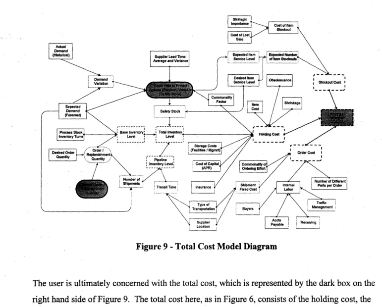
Chapter Preview

In the remainder of this chapter I present the general multi-location, multi-item, inventory management problem, discuss some of the complex issues associated with this problem, show how simpler models can be used to help solve this problem and present a such model. This model is called the "Total Cost Model" as it attempts to fully capture all costs associated with inventory.

This model allows the materials manager to use available data to assist him in his decision making. It serves the dual purpose of allowing the user to evaluate the costs of the system (current or proposed) with an Activity Based Costing methodology and to optimize the decision variables for the selected policy. The model is formulated as an optimization model with the objective function being to minimize cost. However, it has an interface that allows the user to switch off the optimization function and make his own policy decisions so as to evaluate the effects of these. There is also a simulation function which allows the user to visualize the

" Documentation can take many forms. Examples of these forms could be narratives, diagrams, mathematical equations or simple statements of cause and effect.

(34)

II I1

behavior of inventory levels over time and to validate the results of the optimization. The outputs of the model include recommended inventory levels, order / replenishment quantities, expected service level, and expected costs.

General Inventory Management Problem Description

I'll begin by describing the most complex and difficult to manage of inventory worlds. I talk about this for two reasons. First, a major learning for me during my internship experience occurred as I discovered the extreme difficulty involved in attempting to model and optimize such a system. I considered techniques ranging from linear programming to genetic algorithms in a search to find a general solution to a general problem, finally realizing that I had to narrow the problem to make it tractable. Second, I discuss this scenario because, even though

PictureTel's inventory system is not currently so complex, it could become this way if no preventive action is taken. The company should take active measures to ensure it does not unintentionally wind up with such a complex and unwieldy system.

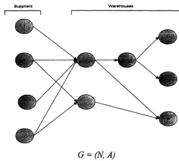
A general multi-echelon inventory system can be modeled as a graph, G = (N, A), which is a

directed network defined by the set N of n nodes and the set A of a directed arcs. Each of the nodes represents an inventory site at which can be stored up to m inventory items, where m is the total possible number of inventory stocking items12

(35)

Suppliers

I 'I

Warehouses

G=(N,A)

Figure 4: General Multi-Echelon Inventory System

At each inventory site, items are stored to satisfy demand from downstream locations. Items are removed from inventory and shipped to satisfy the demand. Items are added to inventory as they arrive from upstream locations. There is some time that elapses between the placement of the order and the arrival of the item. We refer to this time as the lead time. Demand is stochastic as are lead times.

For a single inventory location, I will consider a type of system that requires two decisions to be made for each item at each node: the quantity of inventory carried"3 _{and the lot size ordered.}

13 A note on inventory: For a given planning period, the total planned inventory can be broken into two

classifications. The first is that inventory that is held to meet the expected demand, i.e. the forecast of demand for that period of time. The second category is that inventory that is held to protect against random variations in supply and demand, i.e. given that our forecast will always contain some error, and that there is some cost associated with not having the inventory in stock (underage or stockout cost) and some cost associated with having too much inventory in stock (overage cost) we wish to carry an amount of inventory, called safety stock, that minimizes our total cost for that period. Typically the underage cost is greater than the overage cost, i.e. the cost to the company of not having a piece of inventory on hand when the customer wants it is greater than the cost of carrying that piece of inventory, for one period, in the case that the customer doesn't want it. In this case, we would want to have on hand a positive amount of safety stock. So in each planning period, the total amount of inventory at the beginning of the period is equal to the expected demand plus the safety stock. Since the expected demand will always be ordered, the only real decision variable is the quantity of safety stock.

Page 35

(36)

When the inventory level is being monitored continuously (as opposed to periodically) we refer to the system as being under continuous review. The advent of modem information technology systems has made continuous review inventory control systems very practical as computers can be programmed to generate an alert message, or even a purchase order, when an inventory item drops below a determined level. The type of inventory control system I have described is

referred to as a continuous-review, order-point, order-quantity inventory control system. It is

also referred to as a (Q, r) system where

Q

is the order quantity and r is the safety stock. The order point, R, is the sum of the safety stock and the expected demand over the lead time. This inventory control policy is illustrated in Figure 5: Inventory Level Over Time with (Q,r) Continuous Review Control. When the inventory level drops below the reorder point, R, an order is placed for the order quantity,

Q.

We expect the inventory level to be at r when the order arrives, since we anticipate only the expected demand to be consumed over this lead time

interval. However, since both the demand and lead times are stochastic, the inventory level at the time of order arrival is itself a random variable. From time to time this inventory level will drop below zero before the order arrives. This creates a backlog condition and it is in these situations that the company incurs a stockout cost"4

Inventory Level

me

Figure 5: Inventory Level Over Time with (Q,r) Continuous Review Control

14 For further discussion of these inventory models see Silver, 1979; Nahmias, 1993; Taha, 1987 i i i I!

(37)

We make inventory control decisions with the ultimate goal of maximizing the profitability of the company. Profit is the difference between revenue and cost. Some decisions that we make

concerning the inventory system may have effect on both revenue and cost. For example, say we choose to not carry any inventory of a certain item. In this case we will have no cost associated with holding that item, but neither will we have any revenue from its sale (assuming that since we did not carry it, we could not sell it) resulting in a net profitability, for that item, of zero dollars. Since our inventory decisions have effect on both revenue and cost, if we characterize the costs properly, we can achieve the result of maximizing profitability by minimizing cost. We do this by assigning a cost to lost revenue. This maximization of profitability by the

minimization of cost is the approach I shall take throughout this thesis in considering inventory decisions.

Types of Inventory Costs

All of the costs associated with the inventory system may be grouped into three categories:

* order costs * holding costs * stockout costs

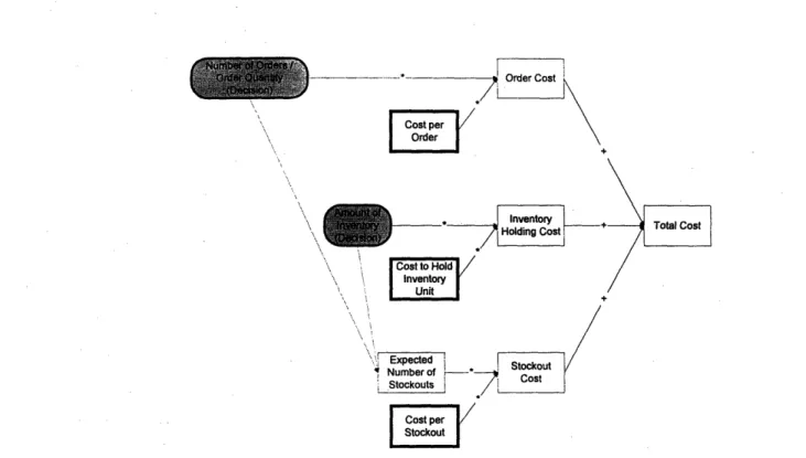
The relationship between these costs and the decisions we can make about inventory are shown, below, in Figure 6. As mentioned above, the decisions we can make concern only the level of

inventory carried and the lot size ordered. As mentioned in footnote 13, when making our inventory level decisions we really are only making a decision about the level of safety stock. The other decision we make concerns the lot size for each order. Since we are assuming some finite level of demand, this is equivalent to specifying the number of orders per time period. I will refer to the safety stock level, r, and the number of orders or order quantity, Q, as decision

variables. We note from Figure 6 that the expected number of stockouts is determined solely by

the decision variables.

(38)

Ii I! Order Cost Cost per+ Order ,..4. Expected _ Stockout Number of Cost Stockouts Cost per Stockou

Figure 6: Relationship Between the Costs of Inventory and the Decision Variables

There is some cost associated with holding an item of inventory at each location per time period, this is referred to as the holding cost. The holding cost includes the cost of capital, the cost of insurance, the cost of warehousing facilities the cost of shrinkage and the cost of obsolescence. There is some fixed cost associated with placing an order for an item from an upstream location, this is referred to as the order cost. The order cost includes the time spent by all employees to place and receive the order and any fixed cost imposed by the supplier and/or the shipping

company. There is some cost associated with failing to satisfy demand for an item, this is

referred to as the stockout cost. The stockout cost includes the lost revenue and customer ill will. As shown in Figure 6, the total cost is the sum of these three costs.

Minimizing Total Cost

As many authors have shown, the task of minimizing inventory costs can therefore be formulated as an optimization problem where we are minimizing the total cost. A mathematical formulation of this optimization problem formulated for a single item at a single location over one year is presented below in Equation 1.

(39)

D

Q

D Min TC(Q,r) = S + IC Q + ICr + - ksN (z)

Q

2

Q

Equation 1 where z

=

r_s S and

D is the annual demand [items]

Q

is the order quantity [items/order] S is the order cost [$/order]

I is the inventory carrying cost as an annual percentage [%]

C is the cost of the item [$/item]

r is the safety stock level [items]

k is the stockout cost [$/stockout]

s is the standard deviation of demand over the lead time

N(z) is the unit normal loss function

sN(z) is the expected number of stockouts in an order interval [stockouts/order]

the components of total cost are:

D S = _{annual procurement cost}_[$] Q

IcQ ₌ _{annual carrying cost to meet the average demand}_[$]

2

ICr = annual carrying cost to hold safety stock [$] D

- ksN(z)= _{annual stockout cost}_[$] Q

and thus TC(Q,r) = DS + IC Q+ ICr + -D ksN(z) is the sum of these cost components.

Q 2 Q

We make the assumption that demand is random and stationary.

(40)

I I I:

Multi-Echelon Complexity

The multi-echelon system15, as described above, is a network of n individual inventory sites. At each of these sites up to m inventory items may be stored. Since we have two decisions to make for each item at each site, we have a total of 2mn decision variables. It would be nice if we could simply sum the total costs of each item at each site to come up with the complete inventory system total cost. This would be possible if each inventory item and site was independent of the remainder of the items and sites, but this is not the case. The items and sites are, in actuality, dependent upon each other. Modeling this type of system is very difficult, or, as Silver puts it,

"probabilistic demand ... _{creates extreme modeling complexities in a multi-echelon inventory}

situation." Next I examine some of these complexities.

First let's consider the implications of having multiple-items in the system. With multiple line items on an order, the treatment of stockout costs can become extremely complex. Typically, when an order is being prepared for shipment and it is discovered that there are one or more line items out of stock, a decision will be made to either delay the entire shipment until all items are available for shipment, or to make a partial shipment immediately of the goods on hand and ship the remainder of the items at a later date. This is referred to as a short shipment. The decision about how to ship is usually made after consultation with the customer. In either case, assigning a stockout cost to the items becomes more confusing. Arguments can be made that the stockout

cost should be the same, less than, or greater than the stockout cost for the independent item. Also, if there are multiple items out of stock and the entire shipment is delayed, the stockout cost would not necessarily be the sum of the stockout costs of the individual items.

Next let's consider the implications of having multiple upstream sites that feed a common item into a single site. This is the case when there are several suppliers of an item to one inventory site. For each of these upstream sites there will probably be a different order cost and a different lead time distribution. Multiple suppliers may be retained to maintain price and service

'5 For further information see Graves, 1989; Lee at al., 1992; Magee et al., 1985; Nahmias, 1993; Rosenfield et al., 1980; Shapiro et al., 1985

(41)

competitiveness, or because one supplier possesses insufficient capacity to satisfy all of the demand. The optimization model presented above would need to be expanded to allow these factors to be taken into account.

Another challenge that arises is estimating the distribution of demand over the lead time. Even if we assume a Gaussian distribution we face the challenge of estimating the parameter s, the standard deviation of demand over lead time. As Nahmias says, "in general, it is very difficult to incorporate the variability of lead time into the calculation of optimal inventory policies." There are two reasons for this. First, lead times from a single supplier may not be independent. The lead time for an order may very well depend on the size of the current and recent prior orders.

Second, if we assume that the lead times are independent random variables, such as would be the case if we had several suppliers of a given item, then it is possible for the lead times to cross, i.e. orders may not be received in the same order in which they were received. Equation 1 assumes that the distribution of demand over the lead time interval is Gaussian. In reality, determining the proper distribution of demand over the lead time interval could be difficult. Even if the

demand distribution is Gaussian, the distribution of demand over lead time will not be, if the lead time distribution has a non-zero variance. This distribution will be complex and would be best

estimated from empirical data and then the model would have to be modified to account for this distribution.

Finally let's consider a more general implication of having a complex, interconnected inventory system. This implication is that actions at the sites are no longer independent. Local

optimization by individual sites can result in far reaching negative effects and suboptimal behavior for the system as a whole. These phenomena have been well documented by scholars such as Forrester and Senge from a System Dynamics perspective and Silver from a purely mathematical perspective.

In summary, accurately modeling a multi-echelon, multi-item inventory system is a task that is exceedingly difficult. As Graves puts it, progress in this field has been slow and most of the advances have been made for very specialized situations such as the cases of deterministic

(42)

demand, serial systems with stochastic demand and one-for-one systems with stochastic demand. For more general multi-echelon inventory control problems, most of the work has been focused on two-echelon distribution systems with identical retail sites with Poisson demand processes16_.

A Simpler Model: Single Item, Single Location

As I have pointed out, finding a solution to the multi-item, multi-echelon inventory, cost minimization problem for a realistic inventory system is a virtually impossible task. Indeed, if there were a tractable17 solution to this problem, there would not be inventory management

challenges, as inventory managers could just program a computer to determine the optimal levels of inventory at any given location and time. In reality, managers must grapple with this problem daily.

There are numerous approaches that could be taken to tackling this problem. One approach could be to model the entire supply chain as thoroughly and accurately as possible and use some sophisticated optimization routine to arrive at a good solution. Some companies, such as Digital Equipment Corporation (DEC)8 and AT&T, have taken this approach. During my internship this was also my first approach. I investigated using a software product developed at DEC called the Global Supply Chain Optimizer, which is a mixed integer program that uses penalty costs to arrive at solutions very rapidly. What I found, though, is that a program of this magnitude requires the full time dedication of many employees to maintain and use the model. Unlike DEC, PictureTel can not currently support the use of such a model. They do not have the internal competency in operations research necessary to support the mode, nor does the scope of their global business (yet) justify such an expenditure.

16 Graves,1989

" Ahuja et al., 1993; Cormen et al., 1990; Winston, 1991

(43)

After abandoning this approach, but still desiring to solve this large scale problem with a large scale approach, I investigated the potential of using genetic algorithms"9 _{as a tool for finding a} near optimal solution. I chose this approach because the multi-item, multi-site, inventory problem is full of complex, non-linear mathematical relationships, and genetic algorithms can

provide good solutions to these types of problems as they broadly search the solution space and don't become trapped at local optima20_{. However, I found that this approach, as well, required} too much support within the company for its continued use, and was too sensitive to model structure and parameter accuracy. Most importantly, though, I felt that this approach decoupled the user from the problem too much. The genetic algorithm searches are truly "black box" searches that randomly search the solution space. I felt that PictureTel's problem was of a scope that was best dealt with a modeling technique that heavily involved the user, forcing him to really understand the model, its inputs and assumptions.

"You cannot conceive the many without the one."

--

Plato

In order to effectively deal with this complex problem I have chosen to take the approach of decomposing it into simpler parts. For example, if portions of the system can be decoupled from each other so that they do not affect one another, then they could be treated separately. These

"portions" of the system refer to both the inventory items and the sites. PictureTel's inventory network is structurally simple enough that, with the proper assumptions, we can reduce the inventory control problem to a single item, in a single location, with stationary demand. So we reduce the complex multi-item, multi-echelon system presented in Figure 2 to a group of simple

single-item, single-site systems as presented in Figure 7.

19 Goldberg, 1989

20 The current paradigm is to use a combination of genetic algoritm and hill climbing techniques to locate promising

regions and then quickly locate the local optima.

(44)

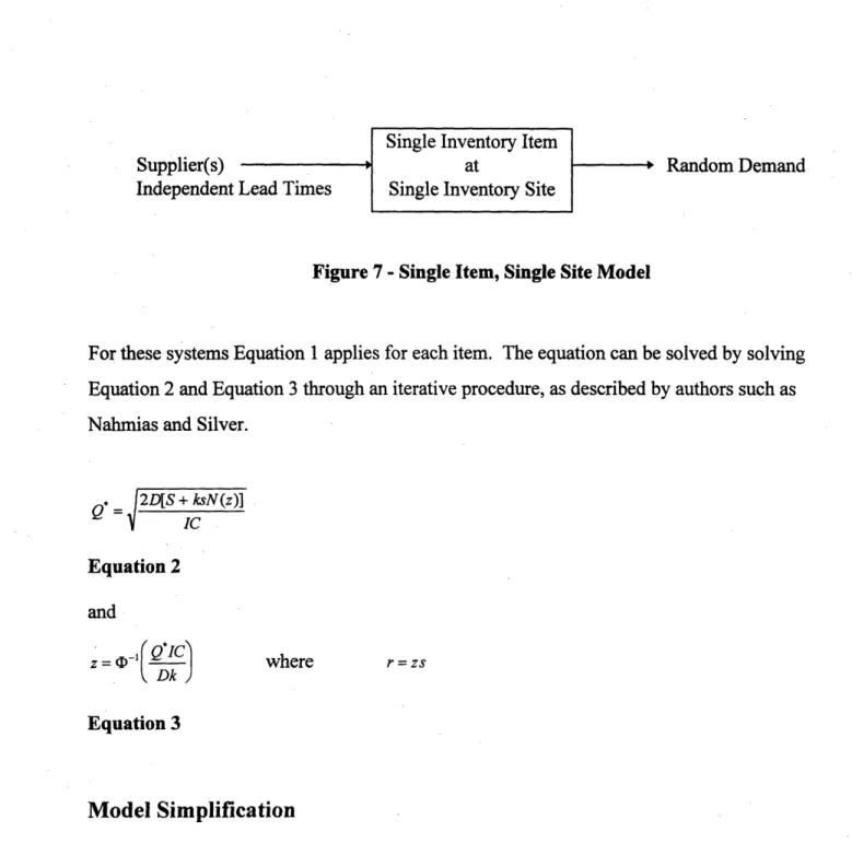
Single Inventory Item

Supplier(s) at Random Demand

Independent Lead Times Single Inventory Site

Figure 7 - Single Item, Single Site Model

For these systems Equation 1 applies for each item. The equation can be solved by solving

Equation 2 and Equation 3 through an iterative procedure, as described by authors such as Nahmias and Silver.

S 2DI[S + ksN(z)] IC Equation 2 and z = c- 'C where r = zs

kDk

Equation 3

Model Simplification

As mentioned above, PictureTel's inventory system can be reduced and this simpler model can be intelligently used to aid in inventory control. I will now explain why this problem simplification is possible, including the assumptions necessary. I will then discuss the model in detail.

(45)

PictureTel Peabody Distribution Center

Even though from an examination of Figure 2 it appears that PictureTel's inventory system is quite long and complex, approximately 90% of the inventory is held in one location, the Peabody Distribution Center (DC). Because the bulk of the inventory is held at this location, this is the

site where the largest potential improvements in inventory control and costs can be made. While the model presented below may used at other inventory sites within the PictureTel supply chain,

in this thesis I will only examine it use at the Peabody DC. Use in other locations would require only the modification of the appropriate model parameters and adherence to the stated

assumptions.

Now PictureTel's inventory system is modeled in the form presented in Figure 8. The interactive effects of the different sites and the different items are assumed to be of negligible magnitude for this model to be valid. I will explain the assumptions made for this approximation and discuss ways to use this model even when items can not be considered independently.

Random Demand Supplier(s)

Independent

Figure 8 -Single Item, Single Site Model

Model Assumptions

The Downstream Distribution Centers (Europe and Japan) Can Be Ignored: Only minimal

quantities (less than 10% of total investment) of inventory are stored at these locations. The biggest cost saving are to be realized at the Peabody DC. For the model to be valid we must have a random demand process drawing inventory from the Peabody DC. This is indeed the

case, as discussed below.

(46)

The Demand at the Peabody DC is Random: The seasonality of PictureTel's sales was discussed in Chapter 1: Introduction and Overview, and graphically depicted in Chart 2. The (historical) aggregate demand can be decomposed into a trend, a seasonal, a constant and a normally distributed random component. A linear regression was performed on the aggregate GSD shipments for a 101 week time period (July 1993 to June 1995). The independent variables that were significant were time, measured as the week of the series (from 1 to 101), thefirst week

of the month, the last week of the month, the last month of the quarter and a special order from a

large customer. These variables capture a good deal of the trend and seasonal components of the demand pattern. The results of the regression are presented in Table 1: Regression Output for Aggregate GSD Shipments July 1993 -June 1995. The residuals are normally distributed. A histogram of the raw residuals is presented in Chart 3 and a normal probability plot is presented in Chart 4. The raw data is presented in Appendix H.

Regression Summary for Total GSD Shipments

R= .8096 R2=- .6554 Adjusted R2

= .6371 F(5,94)=35.8 p<.00000 Std.Error of estimate: 82.3

Ind Var Beta St. Err of Beta B St. Err of B t(94) p-level

Interept 71.28 18.151 3.927 .0002

Time .2386 .0607 1.11 .282 3.930 .0002

First Week of the Month -.1629 .0622 -81.63 31.173 -2.618 .0103 Last Week of the Month .4708 .0691 250.87 36.825 6.813 .0000 Last Month ofthe Quarter .2162 .0664 60.89 18.693 3.257 .0016 Special Order .2729 .0651 372.84 89.018 4.188 .0001

(47)

Distribution of Raw residuals

-300 -250 -200 -150 -100 -50 0 50 100 150 200 250 300 350 400

Chart 3

Normal Probability Plot of Residuals

-150 -50 50 150 250 Residuals Chart 4 350 Page 47 35 30 25 20 0 o %01-0 o 15 z 10 5 0 -250 -_"

Data-driven logistic planning

Data-Driven Logistics Planning

-.

CoIsemeiIU

OFJUL

1TECH6OLOG1996

Eng.

JUL 1 61996

Eg

Table of Contents

Acknowledgments

Chapter 1: Introduction and Overview

Preface

Problem Statement

Background

Company Background

The Videoconferencing Industry

.ilii

ii

ii

,

Systems and Control: Engineering and Business

Inputs

Desired

Output Respt

Output

Procedure for Designing a Controller

Controller Design Procedure

Chapter Conclusions

Overview of the Remaining Chapters

Chapter 2: The Existing State of the Supply Chain

Introduction

Definition of Terms

Material Flow

Local Vendors

Information Flow

Information System

Chapter Conclusions

Chapter 3: Total Cost Model

Introduction to the Model: Dealing with Complex Systems

Chapter Preview

General Inventory Management Problem Description

Q

Q.

Types of Inventory Costs

Minimizing Total Cost

Q

Q

Q

=

Q

Multi-Echelon Complexity

A Simpler Model: Single Item, Single Location

"You cannot conceive the many without the one."

--

Plato

kDk

Model Simplification

PictureTel Peabody Distribution Center

Model Assumptions

_Eng.

_,