Three-dimensional skeletonization and symbolic description in vascular imaging: preliminary results

HAL Id: hal-00804698

https://hal.archives-ouvertes.fr/hal-00804698

Submitted on 26 Mar 2013

HAL is a multi-disciplinary open access

archive for the deposit and dissemination of sci-entific research documents, whether they are pub-lished or not. The documents may come from teaching and research institutions in France or abroad, or from public or private research centers.

L’archive ouverte pluridisciplinaire HAL, est destinée au dépôt et à la diffusion de documents scientifiques de niveau recherche, publiés ou non, émanant des établissements d’enseignement et de recherche français ou étrangers, des laboratoires publics ou privés.

Three-dimensional skeletonization and symbolic

description in vascular imaging: preliminary results

Leslie Verscheure, Laurent Peyrodie, Anne- Sophie Dewalle, Nicolas Reyns,

Nacim Betrouni, Serge Mordon, Maximilien Vermandel

To cite this version:

Leslie Verscheure, Laurent Peyrodie, Anne- Sophie Dewalle, Nicolas Reyns, Nacim Betrouni, et al.. Three-dimensional skeletonization and symbolic description in vascular imaging: preliminary results. International Journal of Computer Assisted Radiology and Surgery, Springer Verlag, 2013, 8 (2), pp.233-246. �10.1007/s11548-012-0784-4�. �hal-00804698�

Three dimensional skeletonization and symbolic

description in vascular imaging

Verscheure L. 1, 2, 3, Peyrodie L. 2, 3, Le Thuc V. 1, N. Reyns1, Dewalle-Vignion A.S. 1, 2, Mordon S. 1, 2, Vermandel M. 1, 2

1

Inserm U703, Université Lille 2, CHRU Lille, 59120 Loos, FRANCE

2

PRESUniversité Lille Nord de France

3

LAGIS CNRS UMR 8146, Université Lille 1, 59655 Villeneuve d’Ascq, FRANCE

Abstract and Key words

This work covers the symbolic description of vascular trees derived from multimodal three dimensional (3D) images. It aims to provide an overall method to analyse such structures, especially in the cerebral vascular tree. As such, it has a clinical application in neurosurgery, particularly in the planning of the surgeon’s gesture.

We have developed a 3D skeletonization method which is adapted to tubular forms and is advisable for symbolic description. The method is based on the construction of the Dijkstra minimum cost spanning tree.

The algorithms were implemented using the laboratory software platform (ArtiMed) and tested on both simulated and clinical data. A specific experimental evaluation plan was drawn up to test the skeletonization and symbolic description methods. This involved testing the methods’ accuracy by calculating the positioning error and its robustness by comparing the results on a series of 18 rotations of the initial volume.

Key words: Medical imaging, vascular network, angiography, 3D skeletonization, symbolic description

1. Introduction

Symbolic description enables a summary to be made of an object observed via imaging, by describing its basic structures (e.g., connected components, branches of vascular trees, pixels, etc.) and the relations existing between its structures. In contrast to segmentation (which only allows a pixel to be classified as “in” or “out” of the object), symbolic description provides an environment in which the object is described according to a hierarchy enabling the exploration of its characteristics ([[[pixel  branch]  connected component]  vascular network]  , etc.).

The human body contains a wide variety of elements which have a tree-like structure with a descending hierarchical organization (mother branches splitting to children branches).The relevance of studying such structures using symbolic description approaches has already been shown for different areas.

In 1993, Gerig et al, [1] proposed an extraction method for 3D structures, in order to represent them using a symbolic approach, where the topological and geometrical information is represented in a tree-like form.

Later, in 2001, Bullit et al [2] highlighted the importance of knowing the relationships between the different branches of the cerebrovascular tree. Their study centered on the neurosurgical context of lower neck tumor resection, where the use of a clamp interrupted blood flow. It showed that understanding the relationships between the different vessels enabled cerebral perfusion to be anticipated and planned for during the operation.

More recently, Megalooikonomou et al [3] have presented a method for characterizing, classifying, and analyzing the similarities of tree-like structures in medical images. Using clinical data obtained from X-ray galactograms, they studied the branching of the lactiferous ducts, combining symbolic representation by graph with “text-mining” techniques. They suggest expanding the potential field of application to the study of links between the form of tree-like structure and the corresponding pathology.

In general, symbolic description has many applications. In the introduction to their article, Palagyi et al, [4] highlight its use in, for example:

- virtual navigation (e.g., bronchoscopy or endovascular procedures), where a descriptive summary of the data allows the treatment linked to the simulation to be optimized

- exploration of complex structures (e.g., cerebral or hepatic vascular networks), which can be simplified as a result of navigation on a graph

- quantitative analysis of tubular forms (e.g., measurement of light or wall thickness) - etc. (this list is not exhaustive)

The implementation of symbolic description usually follows an identical plan, in which the description is obtained after the extraction of data (binarization) and a skeletonization [4;5]. However, no matter the location nor the application, the root of the problem remains in the skeletonization. Much has been written about this subject, including reviews covering methodology [6-14], and its applications in medical imaging [5;15-23].

In this article, we concentrate especially on the cerebral vascular tree. For this location, we studied the minimum cost spanning tree method based on Dijkstra’s algorithm [24]. This algorithm is especially interesting for our application as the search for the centerline uses the notion of the graph.

The first part of this article describes the modalities of vascular imaging, segmentation and 3D reconstruction used in our application. We also describe how we implemented the skeletonization algorithm.

In the second part, we present a new evaluation plan for skeletonization, in which we introduce the use of digital phantoms, as well as tests on clinical data. Finally, we present and analyze the results.

2. Material and methods [25]

As Palagyi et al have noted [4], an overall solution for skeletonization adapted to all types of

locations or forms does not seem to exist. By concentrating on their pulmonary airway tree application, these authors resolved certain difficulties [4], but problems remain for other applications. These problems are mainly linked to the properties defining the skeleton [26]:

- Thickness: the skeleton must have a unitary thickness (one voxel) - Position: the skeleton is ideally positioned at the center of the forms

- Homotopy: the median axis has exactly the same number of connected components, and each component has the same number of holes as the initial form

- Stability: when the skeleton calculation is done by thinning, all or part of the skeleton should not be able to be eroded again once it has stabilized.

Two other properties can also be taken into consideration: - Invariance by translation and rotation

- Reversibility of the skeleton: the form should be able to be reconstructed from the skeleton and the maximum ball rays.

For the vascular application that we are interested in here, we therefore chose to test a method that corresponds in part to the above properties. This method is mainly used for virtual coloscopy, as it is particularly well adapted to tubular forms [24]. It is based on the construction of the Dijkstra’s minimum cost spanning tree.

Our implementation followed the plan generally accepted in the literature [5] for skeletonization and tree extraction, represented as a graph (Figure 1).

- Segmentation of data - Choice of the root

- Skeletonization of the segmented data

- Identification of the skeleton’s branches and nodes - Generation of the tree-like structure as a graph - Tree partitioning

- Quantitative analysis

2.1. Segmentation

The segmentation solution used to extract the vascularization from the images has been described in [27-29]. This algorithm is particularly useful in our case as it allows the independent segmentation of the magnetic resonance angiography (MRA) images with or without injection of contrast agent. The method is based on the analysis of maximum intensity projection (MIP) images. For each voxel, a degree of membership is calculated by integrating the gray level of its projection on the MIP and the contrast to noise ratio (CNR) of the original images (Eq. 1 - Figure 2).

Figure 2: Description of the algorithm based on maximum intensity projection. GlV(x,y,z) is the gray level

at the (x,y) (x,y) position of the slice Z, and GlMIP(x,y) is the gray level of the projection of voxel (x,y,z) on

the maximum intensity projection. The two values are combined to determine if the voxel belongs to the vascular tree (Eq. 1).



where



voxel intensity, GlMIP(x,y) is the intensity of the pixel corresponding to the projection of the voxel on the MIP, WZ is a weighting factor (Eq. 2) allowing the signal to noise relationship of the slice Z to be taken into account.

Wz is determined from equations 2 and 3.

WZ = 1 - exp(-  . CNRZ) Eq. 2

where CNRZ is the CNR measured on slice Z, α is fixed at Log(100)/CNRMax in order to have

Wz = 0.99 for the zones of maximum CNR thus giving them the most reliability.

))² , ( ( ))² , ( ) , ( ( max min max y x Gl y x Gl y x Gl Gl Gl Gl CNR Sx Sy ZF Sx Sy ZF Z z





where the CNR of slice Z is estimated from the maximum and minimum intensities of the slice (cf. Glmax and Glmin), (Sx, Sy) represent the size of the slice, GlZ(x,y) is the gray level at

position (x,y) of slice Z and GlZF(x,y) is the gray level at the same position after filtering using

an averaging filter unit (size 3x3, coefficients=1; normalization factor 1/9). Note that, following the principle of MRA, Glmax and Glmin are situated in the vascular structure and in

the background of the image, respectively.

Once the degree was calculated for each voxel, a binary volume (Figure 3b) was obtained, by retaining the voxels with a degree superior to 0.5. The contour of the vascular tree that was obtained on each slice was then used to refine the form (Figure 3c), using the algorithm described in [27;30].

Finally, note that the use of the MIP limits the use of the method to images in which the vessels are seen in hypersignal, i.e., TOF MRI or Gadolinium contrasted sequence, Computed Tomography Angiography (CTA) or 3D Rotational Angiography (3DRA).

(a) (b)

(c)

Figure 3: Example of segmentation using the algorithm described in [27;30], on MRA images with injection of Gd, from a patient presenting with an intracranial aneurysm, (a)

MIP image obtained from initial study, (b) binary volume obtained after segmentation, (c) volume-rendered view of the aneurysm after the algorithm described by Vial et al [30]

After segmentation, we analyzed the connected components in order to eliminate residual noise. The components with a low number of related voxels were therefore eliminated from the vascular structure before skeletonization.

2.2. Identification of the root

Our study was carried out on the cerebral vascular network, but it can be extended to any tubular structure. The automatic detection of the root, or the Source point, was carried out by distance measurement. The root will obviously be at one end of the tree structure. The automatic algorithm chooses an arbitrary point (centered on the volume) from which the distance to all the form’s voxels is calculated. The point furthest away will be the Source point (Figure 4).

Figure 4: Determination of the Source point

2.3. Skeletonization using Dijkstra’s tree

Skeletonization is the standard method used to determine a form’s centerlines. In continuous or discrete fields, the choice of methods is fairly varied. However, one of the problems that is frequently encountered is the presence of surfaces or small barbules (especially of clusters of voxels at the level of junctions) in a skeleton that we would prefer to be thin [31]. This constraint can be solved by using Dijkstra’s minimum cost spanning tree to extract the thin branches.

This solution for skeletonization, introduced by Wan et al [24] for application in virtual coloscopy, has also been used by Hassan et al in the setting of vascular analysis of aneurysms [32;33]. However, in these articles, the authors used this skeletonization stage with the aim of extracting only one part of the tree: the central colonic axis in [24] or the branches affected by an aneurysm with the intent of carrying out “Computed Fluid Dynamic simulations” [32;33].

Initial point centered on the form

Furthest distance Source point

In the first case, the technique used only allowed the extraction of the principal centerline. In order to extract the first generation branches, the authors therefore proposed an extension to the algorithm from this centerline [24].

In our context, the extension proposed in [24] proved to be inadequate, and we therefore propose a new extension in order to skeletonize the tree down to the most distant vessels. In this generalization, it is advisable to reiterate the process for each first generation branch (see Figure 5) associated with the centerline.

Figure 5: Representation of intergenerational relationships

This new extension can be broken down into 3 stages. Firstly, the Dijkstra’s minimum cost spanning tree was constructed (as described below, 2.3.1); secondly, the principal branch was extracted; finally, the first generation child branches are extracted, followed by the later generations.

2.3.1. Construction of the minimum cost spanning tree

In graph theory, Dijkstra’s algorithm is used to resolve the shortest path problem. It applies to a related graph in which the weight linked to the edge is positive or nil.

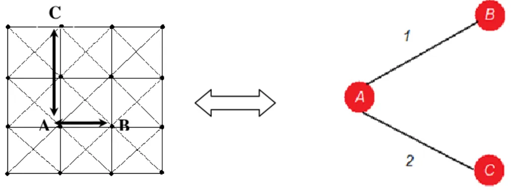
Firstly, the volume had to be converted into a weighted 3D graph. The centre of each voxel therefore represented a node in the graph (Figure 6) and the relations of 26-neighborhood between the voxels are symbolised by the ridges of the graph.

In our case, the weight attributed to each apex is inverse to the distance with respect to the boundary (1/Distance from Boundary [DFB]). The further the voxel under consideration is from the boundary, the higher the probability is that it will be on the centerline, and 1/DFB will therefore be smaller. To calculate the DFB, we calculated the smallest Euclidian distance between each voxel and the boundary points.

Figure 6: 2D representation of a weighted 3D directed graph, where A and B are 2 voxel-nodes with an attributed weight of 1/DFB. The two-directional arrow represents the branch joining nodes A and B.

Next, a sub-graph was progressively built. The different apices were classed in ascending order according to their minimum distance to the Source point (which was chosen as the starting apex). This distance corresponds to the sum of the weights of the borrowed ridges. This step therefore allowed the neighborhood links to be plotted between each voxel, and the attribution of a weight to each link corresponding to its distance from its neighbors. This is illustrated for a 2D form in Figure 7.

To plot the shortest pathway to the Source point, we read the tree inversely, passing from closest neighbor to closest neighbor. We then allocated each voxel in the pathway a link towards its closest neighbor (a pathlink).

Figure 7: The initial volume (left), the corresponding Dijkstra tree (centre), and the two images superimposed (right). An example of a 2D case.

To describe the algorithm, we define the following variables: - Node S: source node

- Node C: node being processed at a given iteration - N/Ni represents a neighbor of Node C

- EndPointList/JunctionList: lists storing the endpoints and the junctions of the detected branches, respectively.

Every node has several properties:

- pathlink: indicates the link with the neighbor (see Figure 6: pathlink(A)=B)

- Distance from source (DFS): is the distance from the node to the source node (taking Figure 6 as an example, if A is the source node, DFS(A)=0, DFS(B)=1, DFS(C)=2, etc)

- the state of the node indicates if it has already been processed during an iteration (Mark (C) = true if processed, otherwise false).

A B

From these definitions and using a heap to process the nodes, the algorithm is described Figure 8:

Figure 8: Algorithm for the calculation of Dijkstra’s tree, where the principal stages are to a) mark point S (mark(S)=true), define it as the current node (C=S), set its pathlink at NULL, and its

distance in relation to the source (DFS, Distance From Source) at 0;

b) stack (push) the neighbors Ni of node C if mark (Ni)=false, and initialize pathlink(Ni)= C, to calculate their distance to node S: DFS(Ni)=DFS(C) + dist(Ni,C) where dist is the Euclidian distance;

c) Pull from the head of the heap in order to process a new node as of stage b)

2.3.2. Extraction of the centerline and its branches using Dijkstra’s tree The centerline extraction algorithm was based on the movement through the tree from the node at maximum DFS up to the Source point. By using each apex’s pathlink property and considering the tree as an oriented graph (in which reversing is impossible), the centerline was defined as the longest branch. The identification of the apex of the maximum DFS is enough to enable a gradual retracing up to the Source apex (chosen in section 2.2), via the pathlinks. The extraction of first generation branches was based on the following stages:

- sweeping through the centerline by retracing from E to S (see Figure 9) along the pathlinks

- for each voxel C of the centerline, looking at its neighbors (apart from those not belonging to the centerline) and finding the Ni’s which have their pathlink at C (e.g., pathlink(Ni)=C)

- for every Ni, searching for all its linked voxels V (either directly pathlink(V)=Ni) or indirectly pathlink(pathlink(…pathlink(V)))=Ni).

- storing Ti as the tip of the branch (i.e., Ti  EndPointList) if DFS(Ti) was above a fixed threshold L for the length of the branch (see Discussion). The length of the branch was calculated by DFS(Ti)-DFS(C).

- storing C as being a junction (i.e., C  JunctionList)

Figure 9 shows an example of searching for a branch, in 2D. Figure 10 summarizes the method.

Figure 9: Extraction of the centerline and its branches. S and E are the source voxel and the end voxel, respectively; C is the current voxel, and Ti is the end voxel of a secondary branch Bi.

Figure 10: Extraction of branches using Dijkstra’s tree. Branch extraction makes use of Branch detection to detect the branches indirectly connected to the current voxel.

A unique characteristic of our algorithm is the storing of the tips of the branches, as appropriate, in the EndPointList or JunctionList. This enables the simultaneous interpretation of the information gathered, both for the preliminary stages of symbolic description and for skeletonization.

After this stage, we extracted the first generation child branches, i.e., the child branches directly linked to the centerline. For the extraction of more distal branches, we chose to implement the algorithm in a recursive manner; this enabled the detection of 2nd, 3rd, and later generation branches, for every extracted branch. The implementation of this new overall method is illustrated in Figure 11.

Figure 11: Recursive skeletonization

The extraction of the 2nd generation branches and onwards was based on the same principle as for the 1st generation. The minor modifications required in the algorithm were:

- sweeping the child branch from Ti to C while retracing from E towards S along the pathlinks

- storing Ti as the branch tip (i.e. Ti  EndPointList) if DFS(Ti) was above a fixed threshold L of the length of the branch (see Discussion). The length of the branch was calculated here as the number of voxels belonging to the branch.

2.4 Identification of particular points

After the skeletonization of the 3D volume, the identification of the different branches was carried out in the classic manner via the analysis and classification of the voxels belonging to the skeleton.

On a skeleton, we can identify three types of points: the endpoints (which have only one 26-neighbor), the junctions (which have exactly two 26-neighbors) and the skeleton points (which have more than two 26-neighbors) (see Figure 12).

Figure 12: Definition of the branches or vascular segments. A branch is defined as the group of voxels situated between an endpoint and a junction, or a junction and another junction; an endpoint is defined

as a voxel with only one neighbor; a junction is defined by the presence of 2 neighbors.

The detection of end points and junctions enables every branch or vascular segment to be defined. There are 3 cases if one compares the skeleton to an oriented graph:

- a branch beginning with an endpoint and ending with a junction: mother branch E-J

- a branch beginning with a junction and ending with a junction: intermediate child branch J-J

- a branch beginning with a junction and ending with an endpoint: end child branch J-E.

From the analysis of Dijkstra’s tree as described above, we already had the skeleton’s characteristic voxels in the EndPointList and the JunctionList. This specificity of the algorithm results in an appreciable reduction in the manipulation of the voxel matrix, and thus reduces calculation time.

However, as our algorithm functions in a recursive way, we extract only the E-J branches. The detection of child branches is carried out as one proceeds, and it is only possible to have a temporary identification of the branches as principal or secondary branches, as such. Each branch then has to be divided into mother, intermediate branch or end branch, according to the cases described above.

2.5 Partitioning of the vascular tree and associated measures

From the skeleton and the branches that were previously extracted, we now wanted to partition the segmented volume voxels into branches, i.e., to link every voxel to a branch in

the skeleton. The method took the segmented volume and the data gathered from the skeletonization (i.e., the skeleton and particular points) as input. As output, the result was a volume for which every voxel was labelled, depending on the branch it belonged to.

Partitioning was carried out automatically by calculating the distances between every voxel in the volume and the voxels in the skeleton. For a given voxel, we searched for the nearest skeletal voxel (which had already been labelled during the skeletonization). The unlabeled voxel was attributed the same label as the skeletal voxel.

Figure 13 shows the result obtained on an artificial volume and a vascular network:

Figure 13: Partitioning of an artificial volume and a vascular network taken from clinical data

Using the formula for the volume of a cylinder, this stage also allowed us to calculate the theoretical radius of each branch. Once the voxels were labeled, we knew the list of those belonging to each branch. Assuming that the vessels could be modeled as cylinders, all that was needed was to calculate the volume corresponding to the group of these voxels and the number of voxels in that branch of the skeleton. These values correspond to the volume (number of voxels  size of voxel) and the length (number of voxels in the branch) respectively of the theoretical cylinder representing the vessel. Therefore:

longueur volume rayon   2.6 Symbolic description

At this stage of the procedure, we could describe the vascular tree as an oriented graph, as we knew the origin and end of the branches, the associated skeletal voxels, the length of the branches, etc. (Figure 14).

Figure 14: Representation of the relationship

A structural representation of the tree is easily obtained, where the object “branch” encompasses various pieces of information (see Figure 15):

- branch hierarchy (index in the list of branches) - the list of voxels associated with the branch - its particular voxels (end voxels and junctions)

- extended relationships (ascending and descending branches) - its radius

- its length

3. Experimental methods

Few methods exist for the evaluation of skeletonization algorithms. However, Palagyi et al [4] have proposed an interesting plan for the quantitative evaluation of skeletonization. Using a physical phantom, a digital phantom, and in-vivo acquisition, their experimental plan enables the number of branches detected, the positioning error, and the diameters, lengths, and volumes of the detected branches to be verified. We adopted approximately the same evaluation strategy in our study.

3.1. Validation criteria 3.1.1. Accuracy

To verify the accuracy of our solution for skeletonization, we compared the skeleton endowed with the characteristics extracted using our method with a theoretical skeleton. This involved examining the skeleton’s positioning error and the precision of the symbolic description information.

3.1.2. Robustness

The second evaluation criterion was the robustness of the symbolic description, i.e., the extent to which the results remain stable after any disruption. The conditions under which images are acquired cannot be exactly the same (especially concerning the orientation of the patient’s head). However, in images from the same patient, the symbolic description should give the same result. We therefore decided to observe how the method dealt with a series of rotations. 3.2. Experimental plan

3.2.1. Accuracy

In the absence of ground truth concerning clinical data, we tested the accuracy of our method on simulated data, using a digital phantom constructed using Matlab© (The MathWorks™, http://www.mathworks.fr). This allowed us to have the geometric information concerning the branches, and as a result, we had the ground truth associated with the volume created (the construction spline of the volume and related information). We then estimated the positioning error, calculated by a hyperbolic Hausdorff distance [34] between the reference skeleton and the obtained skeleton.

To this evaluation, we added the calculation of the Dice Similarity Coefficient (DSC) between the original volume and the reconstructed volume, which allowed us to assess the skeleton’s reversibility properties.

The reconstructed volume resulted from information from the skeleton and the symbolic description. For each point in the skeleton, we thus formed a ball of radius which corresponded to the Euclidian distance between this point and the edge of the nearest volume (DFB).

3.2.2. Robustness

Following Palagyi et al’s approach [4], we rotated each volume studied by 5° from -15° to 15°. This enabled us to study the following characteristics of the branches by opposing the values obtained with or without rotation:

- length - volume - surface - radius

For the statistical analysis, we used the Bland-Altman approach [35;36] for evaluating the agreement between two methods. This method is used to compare two methods in the absence of a gold standard. The aim is to characterize the coherence of the results obtained by the new method compared with those using the other method. We evaluated the reproducibility by comparing the results obtained from the original volume with those of the 18 rotations.

3.2. Data presentation 3.2.1. Simulated data

We created an interface using Matlab (Figure 16 (a)) which allowed us to generate digital models from a reference skeleton (the spline). Secondary branches were connected to a principal branch, forming the skeleton of a tree-like structure. A volume was then constructed from the skeleton and the given branch diameters.

(a) (b)

Figure 16: (a) The digital model’s creation interface enabling the evaluation of the skeletonization algorithm and the symbolic description (b) Resulting digital model

The digital model built up in this way, Figure 16 (b), allowed us to precisely define the characteristics of the skeleton under research: the point coordinates, the radii, the length of branches, relationships, etc..

3.2.2. Clinical data

The clinical data were images taken from different MRA and 3DRA sequences. The sizes were 345x259x142 (MRI, Time Of Flight), 272x188x270 (MRI, Gadolinium Contrast Enhancement), 256x256x150 (MRI, 3D Phase Contrast) and 256x256x256 (3D X ray Rotational Angiography).

4. Results

The algorithms were implemented using a software platform owned by ArtiMed laboratory, and developed in Borland C++. The manipulations were carried out on a personal computer (processor: AMD 2.4 GHz- RAM: 2Go).

Initial volume Skeleton Reconstructed volume

(a) (b) (c) (d) (e) (f)

Figure 17 shows the results on digital phantoms (a-b) and on four clinical cases (c, d, e and f). The initial volume is shown, along with the skeleton extracted using our method, and the volume reconstructed from the skeleton.

4.1. Accuracy

As previously mentioned, we indicated the hyperbolic Hausdorff distance between the skeleton obtained using our approach and the construction spline. In addition, for the 18 rotations of the Matlab volume, we determined the mean DSC between the reconstructed volume and the original volume.

Figure 18 shows the visual and quantitative results obtained on two digital phantoms using our algorithm for model generation. The images represent the superimposition of the initial skeleton on the calculated skeleton, and the initial volume superimposed on the volume obtained after post-skeletonization reconstruction. The numbers given are the mean values of the hyperbolic Hausdorff distance and the DSC from the 19 volumes.

Skeleton/Spline Reconstructed volume/Original volume

(a)

(b) 15.36 76%

(c)

(d) 16.22 72%

Figure 18: Results on digital phantoms (a-c) Superimposition (reference in green, results in red) (b-d) Numerical results: hyperbolic Hausdorff distance and Dice Similarity Coefficient

4.2. Robustness

For each branch extracted by symbolic description, we compared a given characteristic of the initial volume (length, radius or number of voxels in the branch) with the same characteristic in the reconstructed volume after rotation and extraction. For each rotation and each branch, we therefore obtained the percentage error of the characteristic studied, denoted by err_vali,j,

For each characteristic, we then calculated the mean error on all rotations on each branch, using:

Finally, the mean percentage error for each characteristic was described by:

Table 1 shows the mean percentage errors ± SD for the reproducibility of the characteristics studied between the original volume and the 18 volumes obtained by rotation.

Table 1 : Reproducibility of results: quantitative data

The reproducibility indices for the radius and the number of voxels on the simulated data are shown in Figure 19; the corresponding indices for two clinical cases are shown in Figure 20. The Bland-Altman plots indicate the 95% Confidence Intervals.

For each case, the mean difference between the estimates obtained from the 2 methods is represented, according to the mean of the two estimates, m1 and m2. When there is no additional information, this mean represents the best estimate of the true value of the parameter. In our case, the m1 estimate was replaced by the values obtained for the initial volume, and the m2 estimate took the values resulting from each rotation alternately.

On this type of plot, the mean of the differences corresponds to the mean bias between the two methods. If one hypothesizes that the differences follow a normal distribution, 95% will be between the mean value ± 1.96 x SD of the differences. According to this interval’s range, one can determine if the two methods are interchangeable. For example, a maximum tolerable value of difference can be fixed, so that the methods can be used to replace one another. We then studied the reproducibility of the characteristics (branch length, number of voxels per branch and the radius of branches for the 19 volumes [initial volume + 18 rotations])

For i=1, …, number of branches For j=1, …, number of rotations

100 * _ _, init rot Init j i val val val val err j   end end Eq. 4

For i=1, …, number of branches

)

_

(

_

_

i

mean

err

val

val

err

my



Volume ( a) D iff ere nce in voxels [% ] D iffere nce in l ength [vo xel] Volume (b) D iff ere nce in voxels [% ] D iffere nce in l ength [vo xel]

Figure 19: Reproducibility of results on simulated volumes: Bland-Altman plot

-35 -25 -15 -5 5 15 25 35 0 1000 2000 3000 4000 -10 -5 0 5 10 0 20 40 60 80 100

Mean number of voxels in a branch [voxel]

Mean length of a branch [voxel] Volume moyen des

branchesvoxel]

Volume moyen des branches [voxel] Volume moyen des branches [voxel] -10 0 10 20 0 100 200 300 400 500 biais data intervalle sup intervalle inf

Longueur moyenne des branches [voxel] Mean length of a branch [voxel]

Reproducibility of number of voxels Reproducibility of the length Volume (c) D iff ere nce in voxels [% ] D iffere nce in l ength [vo xel] Volume (b) D iff ere nce in voxels [% ] D iffere nce in l ength [vo xel]

Figure 20: Reproducibility of results for clinical data: Bland-Altman plot

-30 -20 -10 0 10 20 30 0 10000 20000 -20 -10 0 10 20 0 100 200 300 400 500 -30 -20 -10 0 10 20 30 0 10000 20000 30000 -50 -40 -30 -20 -10 0 10 20 30 40 50 0 100 200

Mean number of voxels in a branch [voxel]

Mean length of a branch [voxel] Volume moyen des

branchesvoxel]

Volume moyen des branches [voxel] Volume moyen des branches [voxel] -10 0 10 20 0 100 200 300 400 500 biais data intervalle sup intervalle inf

Mean number of voxels in a branch [voxel]

Longueur moyenne des branches [voxel] Mean length of a branch [voxel]

5. Discussion

5.1. Analysis of the method

The method that we have proposed for the extraction of centerlines and the descriptive analysis of tubular objects has several interesting properties. Firstly, the basic tool for the calculation of the skeleton is the construction of Dijkstra’s tree. This enables a thin result to be obtained (1 voxel thick) without the need of a pruning stage, as a length limit is applied during the branch detection phase. Secondly, the use of this approach to skeletonization allows a preliminary description to be carried out “during the extraction”. The iterative detection of the skeletal branches enables a first analysis of the tree structure.

The accuracy of our method was evaluated only on simulated data, for which we knew the ground truth of the construction. We could see the good superimposition obtained between the skeleton and the construction spline, with a hyperbolic Hausdorff distance of 15 voxels. We can conclude that, on the simulated data, the method is satisfactory, as the value of 15 (which notably reveals non-detection of the smallest branches) is highly acceptable, given the severe criteria chosen. In the same way, we evaluated the accuracy using the skeleton’s reversibility criteria, by superimposing the original volume on the reconstructed volume. The DSC was chosen to quantify the superimposition, and the mean value obtained was 76%. Taking into account our spherical reconstruction model, and the use of the mean radial value of each branch, we conclude that the index of 76% indicates good reversibility. In fact, the theoretical index calculated for the reconstruction method used after symbolic description versus the volume obtained by the model generator gives a maximum value of 90.7%. This value highlights the shortcomings in our reconstruction model, but enables the value obtained during the experiments to be more clearly analyzed and understood.

Turning to the robustness, we first presented the means and SDs of the percentage errors for each characteristic (length, volume and radius of the branches). Apart from that of the radius, the error SDs obtained were small and therefore highly satisfactory. Taking into account the characteristics extracted by symbolic description, the error obtained for the radius was not satisfactory; this error concerned the mean radius of a branch and did not take into account the variability which exists along the branches. However, no matter which characteristic was studied, the use of the Bland-Altman plots enabled us to observe that 95% of the points were within the confidence interval, thus implying that the method was robust with regard to the volume orientation before skeletonization and symbolic description.

5.2. Limits of the skeletonization method

Since the result of Dijkstra’s algorithm is an oriented graph without cycle, it is not easy to detect and delete the holes (loops in the graphs). As a result, although our method is satisfactory in the majority of cases, it creates a problem when dealing with the intracranial network: the circle of Willis is a loop which is incompatible with the method as it exists.

A preliminary study of the different general methods of 3D skeletonization enables us to suggest a solution to this problem. The Distance-ordered Homotopic Thinning method, proposed by [37], seems to be able to resolve the problem in this localised area (Figure 21). However, as it does not integrate the descriptive data as does our method based on Dijkstra’s algorithm, this other

skeletonization method is generally less appropriate for our symbolic description application. It would be reasonable to envisage associating the 2 methods.

(a) (b)

Figure 21: Descriptive graph obtained of circle of Willis using synthetic data (a) Proposed method (Dijkstra) (b) Distance-ordered Homotopic Thinning method

5. Conclusion and future prospects

We have proposed a new approach to the extraction of the cerebral vascular tree based on the calculation and analysis of the Dijkstra’s minimum cost spanning tree. Furthermore, we have proposed an original framework for evaluation which is adapted to all types of tubular forms (blood vessels, lactiferous ducts, the pulmonary network, etc.).

Our method of symbolic description enables the analysis and interpretation of a vascular network obtained from angiographic images. It provides a simplified representation of the network in the form of a skeleton, as well as a description of the corresponding information in the form of a tree-like view. It therefore creates an interaction between visual and descriptive information by linking these two representations of the network. This type of vessel representation may be of use in the development of new applications (e.g., in new Computational Fluid Dynamics models, or the association of a subject’s data with a vascular atlas, etc.).

A DSC above 70% proves that the skeleton is reversible. In addition, the weak positioning error between the reference and the calculated skeleton indicates that the algorithm is robust. This leads us to conclude that the method is relevant for tree-like objects, and, in particular, satisfies the fundamental requirements needed for future clinical application.

At first, we chose to detect the root of Dijkstra’s tree automatically, without taking anatomical considerations into account. The identification of the tree root could possibly be improved by using anatomical information beforehand, thus allowing the skeletonization to be started on a principal artery, respecting the direction of blood flow.

In the context of the cerebral vasculature, a future application could be the development of supporting software in neurosurgery. By simply clicking on the zone required on the segmented 3D network, the software interface should enable the neurosurgeon to easily identify a branch and its children, and give him or her access to its morphological data (Figure 22).

(a) (b)

Figure 22: Interaction between the view of the tree and the volume. The software extracts the symbolic information at the clicked point (in blue). An inverse interaction is also possible.

Finally, due to a quicker analysis of the network after its description, we envisage the development of a tool which will analyse the interactions between the vascular network and the surgical instruments. This tool could be developed as simulation software to improve the accuracy of the surgeon’s gesture.

Bibliography

[1] G.Gerig, T.Kollera, G.Székely, C.Brechbuhler, and O.Kubler, "Symbolic descriptions of 3-D structures applied to cerebral vessel tree obtained from MR angiography volume data,"

Proceedings of 13th International Conference on Information Processing in Medical Imaging, IPMI'93, ser. Lecture Notes in Computer Science, vol. 687, pp. 94-111, 1993.

[2] E.Bullit, S.Aylward, K.Smith, S.Mukherji, M.Jiroutek, and K.Muller, "Symbolic description of intracerebral vessels segmented from Magnetic Resonance Angiograms and evaluation by comparison with X-Ray Angiograms," Medical Image Analysis, vol. 5, pp. 157-169, 2001. [3] V.Megalooikonomou, M.Barnathan, D.Kontos, P.R.Bakic, and A.D.A.Maidment, "A

representation and classification scheme for tree-like structures in medical images : analyzing the branching pattern of ductal trees in X-ray galactograms," IEEE Transactions on medical

imaging, vol. 28, no. 4, pp. 487-793, Apr.2009.

[4] K.Palagyi, J.Tschirren E.A.Hoffman, and M.Sonka, "Quantitative analysis of pulmonary airway tree structures," Computers in Biology and Medicine, vol. 36, no. 9, pp. 974-996, Sept.2006.

[5] Z.Chen and S.Molloi, "Automatic 3D Vascular Tree Construction in CT angiography,"

Computerized Medical Imaging and Graphics, vol. 27, pp. 469-479, 2003.

[6] L.Lam, S.W.Lee, and C.Y.Suen, "Thinning Methodologies -- A Comprehensive Survey ,"

IEEE Transaction on Pattern Analysis and Machine Intelligence, vol. 14, pp. 869-885, 1992.

[7] C.Kirbas and F.Quek, "A review of vessel extraction techniques and algorithms," ACM

Computing Surveys, vol. 36, no. 2, pp. 81-121, June2004.

[8] T.Saito and J.Toriwaki, " A sequential thinning algorithm for three dimensional digital pictures using the Euclidean distance transformation ," 1995, pp. 507-516.

[9] K.Krissian, G.Malandain, N.Ayache, R.Vaillant, and Y.Trousset, "Model based detection of tubular structures in 3D images," COMPUTER VISION AND IMAGE UNDERSTANDING, vol. 80, pp. 130-171, 2000.

[10] P.Saha, B.Chaudhury, and D.Majumder, «A new shape-preserving parallel thinning algorithm for 3D digital images," Pattern Recognition, vol. 30, pp. 1939-1955, 1997.

[11] S.Aylward and E.Bullit, "Initialization, noise, singularities, and scale in height ridge traversal for tubular object centerline extraction," IEEE Transactions on medical imaging, vol. 21, pp. 61-75, 2002.

[12] M.Maddah, A.Afzali-Kusha, and H.Soltanian-Zadeh, "Efficient center-line extraction for quantification of vessels in confocal microscopy images," Med. Phys., vol. 30, pp. 204-211, 2003.

[13] K.Palagyi and A.Kuba, " A 3D 6-subiteration thinning algorithm for extracting medial lines,"

Pattern Recognition Letters, vol. 19, no. 613, p. 627, 1998.

[15] S.Wood, A.Zerhouni, J.Hoford, E.A.Hoffman, and W.Mitzner, "Measurementd of three-dimensionnal lung tree structures using computed tomography," Application Physiology, vol. 79, pp. 1687-1697, 1995.

[16] K.Mori, J.Hasegawa, J.Toriwaki, H.Anno, and K.Katada, "A fast rendering method using the tree structure of objects in virtualized bronchus endoscope system,", 1131 ed 1996, pp. 33-42. [17] I.Nyström, "Skeletonization applied to magnetic resonance angiography images," Proceeding

of Medical Imaging, vol. 3338, pp. 693-701, 2003.

[18] S.Wan, A.Kiraly, E.Ritman, and W.Higgins, "Extraction of the hepatic vasculature in rats using 3-D micro-CT images," IEEE Transactions on medical imaging, vol. 19, pp. 964-971, 2000.

[19] S.Wan, E.Ritman, and W.Higgins, "Multi-generational analysis and visualization of the vascular tree in 3D micro-CT images," Computers in Biology and Medicine, vol. 32, pp. 55-71, 2002.

[20] K.Mori, J.Hasegawa, Y.Suenaga, and J.Toriwaki, "Automated anatomical labeling of the bronchial branch and its application to the virtual bronchoscopy system," IEEE Transactions

on medical imaging, vol. 19, pp. 103-114, 2000.

[21] J.Toriwaki and K.Mori, "Distance transformation and skeletonization of 3D pictures and their applications to medical images," Digital and Image Geometry, ser. Lecture Notes in

Computer Science 2243, pp. 412-429, 2001.

[22] T.Deschamps and L.D.Cohen, "Fast extraction of minimal path in 3D images and applications to virtual endoscopy," Medical Image Analysis, vol. 5, pp. 281-299, 2001. [23] L.Antiga, B.Ene-Iordache, and A.Remuzzi, "Computational geometry for patient-specific

reconstruction and meshing of blood vessels from angiography," IEEE Transactions on

medical imaging, vol. 22, pp. 674-684, 2003.

[24] M.Wan, Z.Liang, Q.Ke, L.Hong, I.Bitter, and A.Kaufman, "Automatic Centerline Extraction for Virtual Colonoscopy," IEEE Transactions on medical imaging, vol. 21, no. 12, pp. 1450-1460, 2008.

[25] L.Verscheure, L.Peyrodie, N.Makni, N.Betrouni, S.Maouche, and M.Vermandel, "Dijkstra's Algorithm Applied to 3D Skeletonization of the Brain Vascular Tree: Evaluation and Application to Symbolic Description," 32nd Annual International Conference of the IEEE

EMBS, Buenos Aires, Argentine, pp. 3081-3084, Sept.2010.

[26] C.J.Hilditch, "Linear skeletons from square cupboards," Machine Intelligence, vol. 4, pp. 404-420, 1969.

[27] M.Vermandel, N.Betrouni, C.Taschner, C.Vasseur, and J.Rousseau, "From MIP image to MRA segmentation using fuzzy set theory," Computerized Medical Imaging and Graphics, vol. 31, no. 3, pp. 128-140, Apr.2007.

[28] M.Vermandel, AS Dewalle, P.Puech, C.Taschner, J.Rousseau, and N.Betrouni, "MRA segmentation algorithm using MIP and fuzzy set principles. Application to TOF contrast

enhancement sequences," International journal of computer assisted radiology and surgery, pp. 104-106, 2007.

[29] M.Vermandel, N.Betrouni, R.Viard, AS Dewalle, S.Blond, and J.Rousseau, "Combining MIP images and fuzzy set principles for vessels segmentation : application to TOF MRA and CE-MRA," International Conference of the IEEE Engineering in Medicine and Biology Society, pp. 6255-6258, 2007.

[30] S.Vial, D.Gibon, C.Vasseur, and J.Rousseau, "Volume delineation by fusion of fuzzy sets obtained from multiplanar tomographic images," IEEE Transactions on medical imaging, vol. 20, pp. 1362-1372, 2001.

[31] M.Naf, G.Székely, R.Kikinis, M.Shenton, and G.Kubler, "3D Voronoï skeletons and their usage for the characterization and recognition of 3D organ shape," Computer Vision,

Graphics, and Image Processing, vol. 66, pp. 147-161, 1997.

[32] T.Hassan, EV.Timofeev, T.Saito, H.Shimizu, M.Ezura, Y.Matsumoto, K.Takayama,

T.Tominaga, and A.Takahashi, "A proposed parent vessel geometry-based categorization of saccular intracranial aneurysms: computational flow dynamics analysis of the risk factors for lesion rupture.," American Journal of Neuroradiology, vol. 103, no. 4, pp. 662-680. Erratum in: J Neurosurg. 2005 Dec;103(6):1110., Oct.2005.

[33] T.Hassan, M.Ezura, EV.Timofeev, T.Tominaga, T.Saito, A.Takahashi, K.Takayama, and T.Yoshimoto, "Computational simulation of therapeutic parent artery occlusion to treat giant vertebrobasilar aneurysm.," American Journal of Neuroradiology, vol. 25, no. 1, pp. 63-68, Jan.2004.

[34] SW.Choi and HP.Seidel, "Hyperbolic Hausdorff distance for medial axis transform.,"

Graphics Models, vol. 63, no. 5, pp. 369-384, 2001.

[35] D.G.Altman and J.M.Bland, "Measurement in medicine: the analysis of method comparison studies," Statistician, vol. 32, pp. 307-317, 1983.

[36] J.M.Bland and D.G.Altman, "Statistical methods for assessing agreement between two methods of clinical measurement," Lancet, vol. 1, no. 8476, pp. 307-310, 1986.

[37] C.Pudney, "Distance-ordered Homotopic Thinning : a skeletonization algorithm for 3D digital images," COMPUTER VISION AND IMAGE UNDERSTANDING, vol. 72, no. 3, pp. 404-413, Dec.1998.