HAL Id: tel-01477549
https://tel.archives-ouvertes.fr/tel-01477549
Submitted on 27 Feb 2017
HAL is a multi-disciplinary open access archive for the deposit and dissemination of sci-entific research documents, whether they are pub-lished or not. The documents may come from teaching and research institutions in France or abroad, or from public or private research centers.
L’archive ouverte pluridisciplinaire HAL, est destinée au dépôt et à la diffusion de documents scientifiques de niveau recherche, publiés ou non, émanant des établissements d’enseignement et de recherche français ou étrangers, des laboratoires publics ou privés.
Microseismicity around an asperity in the Ecuadorian
subduction zone
Mónica Segovia Reyes
To cite this version:
Mónica Segovia Reyes. Microseismicity around an asperity in the Ecuadorian subduction zone. Earth Sciences. Université Côte d’Azur, 2016. English. �NNT : 2016AZUR4108�. �tel-01477549�
École doctorale: Sciences Fondamentales et Appliquées No. 364 Unité de recherche: GéoAzur UMR 7329
Thèse de doctorat
Présentée en vue de l’obtention du Grade de Docteur en Sciences de la Terre de
l’UNIVERSITÉ COTE D’AZUR Présentée et soutenuée par:
Mónica SEGOVIA REYES
Imagerie microsismique d’une asperité sismologique
dans la zone de subduction Équatorienne
Thèse dirigée par M. Philippe CHARVIS et M. Mario C. RUIZ
Soutenue le 25 novembre 2016 devant le jury composé de:
M. Jordi DIAZ CUSI CR, CSIC, Barcelone Rapporteur M. Serge LALLEMAND DR, CNRS Rapporteur M. Bertrand DELOUIS Professeur UNS Examinateur M. Martín VALLÉE Physicien du CNAP Examinateur Mme. Yvonne FONT CR, IRD Encadrante
M. Philippe CHARVIS DR, IRD Directeur de thèse M. Mario C. RUIZ DR, EPN, Quito Co-directeur de thèse
Abstract
The central subduction zone of Ecuador is characterized by a low interseismic coupling with a small highly-coupled patch centered at La Plata Island. In this region, no large earthquakes have occurred in historical times. However, in the instrumental period, frequent seismic swarms have been observed. Recently two seismic swarms have been observed to occur along with slow slip events. In that sense, for other past seismic swarms there are observations of synchronous displacements observed by GPS that lead to interpret the seismic swarms as accompanying activity of slow slip events. We agree that this might be the characteristic behavior of this zone.
The lack of reliable earthquake locations to image and understand the process behind the slow slip events, leads us to install an offshore-onshore seismic network. The achieved seismic image has no precedent resolution and it help us to characterize the background activity as well as the occurrence and evolution of a slow slip event. For this analysis we beneficiate of the kinematic modeling of the slow slip event by J. M. Nocquet.
The background activity is organized in several clusters. In-land, the clusters are located below the Coastal Range, on the interplate contact zone and in the slab, and they are surrounding the downdip extension of the coupled patch. Offshore, the activity occurs in pre-existing fault structures of the slab that are activated by the accumulated strain related to the highest coupled region (>70 %). The seismicity rate in these two regions seems to be sensible to the occurrence of a medium sized outer-rise earthquake as well as to a slow slip event in the shallow seismogenic zone.
The 2012-2013 slow slip event can be characterized as a composite event made of two zones and two periods of aseismic moment release (sequence) that initiates at the end of November 2012. In the first stage of the sequence, the slip occurs in a small patch (No. 1) in a region of intermediate coupling to the south of La Plata Island with an intermittent, low and slow aseismic moment release (~22% of the total moment released). During this stage that lasted 1.5 months almost no seismicity was detected in the marine forearc and the seismicity rate below the Coastal Range decreased. Then, in mid-January 2013, in the second stage, the slip accelerates in the first patch; synchronous to this acceleration, the seismicity starts in a crustal intraslab fault zone immediately updip of the slipped patch. The next day, abruptly a second patch (No. 2) initiates to move. This second patch is located updip of the first patch in a region of higher coupling which is not supposed to generate SSE. The initial activity on the crustal intraslab fault zone, may have released fluids that change the stability properties of the interface contact zone allowing the onset of the slip on the second patch. The subsequent seismicity: observed migrations and the activation of other intraslab fault zones are caused by the difference in the amount of slip experienced by the two patches where we advocate to a stress transfer effect. During this second stage, the second patch has a limited time of life of 7 days, while the first patch continues to show an
intermittent and small movement until mid-February 2013, with a global moment release equivalent to a magnitude 6.3 Mw.
Our detailed timing analysis let us to propose causal-relationships between slow slip events and seismicity: (i) a stress interaction of slow slip events over intraslab crustal fault zones and (ii) the fluid release from these crustal fault zone over the characteristics of the seismogenic zone that change in few hours from unstable to stable behavior.
The 2012-2013 slow slip event enhances the diversity of SSE in the region. We observe that the accompanying seismicity in the case of the 2012-2013 SSE is almost totally within the subducted plate (drawing up the front of a seamount carried by the Nazca Plate) while for the 2010 SSE it is at the interface. Comparing the aseismic moment release, both SSE are similar and the relative seismic moment release is also comparable.
Finally, taking into consideration that all documented shallow SSE (2005, 2010 and the SSE presented here) release a considerable amount of accumulated deformation with a certain frequency, they may decrease the slip deficit in the region and possibly delaying a major earthquake.
Résumé
La zone de subduction centrale de l'Équateur est caractérisée par un faible couplage inter-sismique avec un petit patch fortement couplé centré sur l'île de La Plata. Dans cette région, on ne connait aucun grand séisme dans les archives historiques. Cependant dans la période instrumentale des essaims sismiques ont été fréquemment observés. Récemment, deux essaims sismiques ont été enregistrés conjointement à l’occurrence des séismes lents. Ainsi, pour les autres essaims passés, cette observation synchrone de déplacement GPS, on conduit à interpréter les essaims sismiques comme une activité accompagnant des séismes lents répétitifs. Nous pensons que ce pourrait être le comportement caractéristique de cette zone.
Le manque de localisations hypocentrales fiables pour l'imagerie et la compréhension des processus aboutissant aux séismes lents, nous a amené à installer un réseau sismologique à terre et en mer. L'image de la sismicité est d’une résolution sans précèdent et elle nous permet la caractérisation de l'activité de fond ainsi que de l'occurrence et de l'évolution d'un séisme lent. Pour cette analyse, nous bénéficions de la modélisation cinématique du séisme lent par J. M. Nocquet.
L'activité de fond est organisée en plusieurs essaims. À l'intérieur des côtes, les essaims sont situés sous la chaîne côtière, sur la zone de contact interplaque et dans la plaque en subduction délimitant la partie profonde de la zone couplée. En mer, l'activité se produit dans des structures préexistantes de la plaque en subduction qui sont activées par l’accumulation de contraintes dans la zone fortement couplée (>70%). Le taux de sismicité dans ces deux régions semble être corrélé à l'occurrence d'un séisme outer-rise de magnitude modéré ainsi que d’un glissement lent dans la partie superficielle de la zone sismogène d’interplaque.
Le glissement lent de 2012-2013 peut être décrit comme un événement composite constitué de deux patches se développant au cours de deux périodes de libération de moment asismique (séquence) qui débute à la fin de Novembre 2012. Dans la première étape de la séquence, le glissement lent se produit sur un petit patch (patch 1) modérément couplé au sud de l'île de La Plata, avec une libération du moment intermittente, faible et lente (~ 22% du moment total libéré). Pendant cette phase qui a duré 1,5 mois, quasiment aucune sismicité n'est pas détectée dans la zone marine et le taux de sismicité sous la chaîne côtière diminue. Puis, à la mi-janvier 2013, dans la deuxième étape, le glissement accélère sur le patch 1; synchrone de cette accélération, l’activité sismique démarre dans une zone de faille crustale intraplaque plongeante situé immédiatement au-dessus du patch 1. Le lendemain, brusquement, un deuxième patch (patch 2) commence à se débloquer. Ce deuxième patch plus superficiel et au nord-ouest du premier patch, se localise sur un zone de très fort couplage qui n'est pas supposé générer des séismes lents. Nous proposons que l'activité de la zone de faille crustale intraslab peut avoir libéré des fluides qui, injectés sur la zone de contact interplaque
auraient modifié les propriétés de stabilité des matériaux présents permettant le glissement sur le patch 2. La sismicité subséquente: les migrations observées et l'activation d'autres zones de faille intraslab sont causées par la différence de la quantité de glissement expérimentée par les deux zones où nous proposons un effet de transfert de contraintes. Au cours de cette deuxième étape, le patch 2 glisse durant 7 jours, alors que le patch 1 continue à montrer un glissement intermittent et faible jusqu'à la mi-février 2013. La libération globale du moment est équivalente à une magnitude de 6.3 Mw.
L’analyse détaillée de l’évolution dans le temps du glissement lent nous permet de proposer des relations de causalité entre ces événements de glissement lent et la sismicité: (i) un transfert de contraintes d’un événement de glissement lent vers les zones de faille crustales intraslab et (ii) la libération de fluide des zones de faille crustales intraslab pour modifier les propriétés de la zone sismogène interplaque en quelques heures, passant d'un comportement instable à un comportement stable.
Le glissement lent de 2012-2013 accroît la diversité de ces types de phénomène dans la région. Nous observons que la sismicité qui accompagne l’événement de 2012-2013 se trouve presque totalement dans la plaque en subduction (délimitant la bordure d’un massif porté par la plaque de Nazca) alors que pour l’événement de 2010, elle est localisée à l'interface. En comparaison, les moments asismiques des deux événements lents sont similaires et la libération de moment sismique relatif associé est également comparable.
Enfin, en tenant compte du fait que tous ces glissements lents superficiels documentés (2005, 2010 and celui étudié ici) libèrent une quantité non-négligeable des contraints avec une certaine fréquence, ils diminuent le déficit de glissement dans la région et peuvent ainsi contribuer à retarder un grand séisme.
Resumen
La zona central de la subducción ecuatoriana se caracteriza por un bajo acoplamiento intersísmico con una pequeña región altamente acoplada centrada en Isla de La Plata. En esta zona no se conocen grandes terremotos en tiempos históricos. Sin embargo, en el período instrumental, frecuentes enjambres sísmicos han sido registrados. Recientemente se han observado dos enjambres sísmicos, junto con la ocurrencia de sismos lentos. En este sentido, para otros enjambres sísmicos del pasado hay observaciones de desplazamientos sincrónicos observados por GPS que conducen a interpretar que los enjambres sísmicos siempre acompañan a los sismos lentos. Coincidimos en que este podría ser el comportamiento característico de esta zona.
La falta de localizaciones fiables de la sismicidad para entender el proceso detrás de los sismos lentos, llevó a instalar una red sísmica tierra-mar. La imagen sísmica obtenida tiene una resolución sin precedentes y ha ayudado a caracterizar la actividad de fondo así como la ocurrencia y la evolución de un sismo lento. Para este análisis se utiliza el modelo cinemático del sismo lento elaborado por J. M. Nocquet.
La actividad de fondo se organiza en dos zonas. En tierra, los enjambres se localizan bajo la Cordillera Costera, en la zona de contacto entre las placas y en la placa subducida rodeando el límite de la zona acoplada. Bajo el mar, la actividad ocurre en fallas preexistentes de la placa subducida activadas por la deformación acumulada relacionada con la región de mayor acoplamiento (> 70%). La tasa de sismicidad en estas dos regiones parece ser sensible a la ocurrencia de un terremoto de magnitud media en la antefosa así como a un sismo lento en la zona sismogénica interplaca superficial.
El sismo lento de 2012-2013 se puede caracterizar como un evento compuesto ocurrido en dos zonas y en dos etapas de liberación de momento sísmico (secuencia) que comienza a finales de noviembre de 2012. En la primera etapa de la secuencia, el deslizamiento ocurre en una zona (No. 1) con un acoplamiento intermedio al sur de la Isla de La Plata con una liberación de momento intermitente, baja y lenta (~ 22% del momento total liberado). Durante esta etapa que duró 1.5 meses casi no se detectó sismicidad en la zona marina y la tasa de sismicidad bajo la Cordillera Costera disminuyó. Luego, a mediados de enero de 2013, en la segunda etapa, el deslizamiento se acelera en la primera zona; sincrónico a esta aceleración, la sismicidad comienza en la placa subducida (zona de falla) inmediatamente al NO de la zona. Al día siguiente, abruptamente una segunda zona (No. 2) comienza a moverse. Esta segunda zona se localiza al NO de la primera, es más superficial y se caracteriza por tener un mayor grado de acople donde se supone que no ocurren sismos lentos. La actividad sísmica inicial en la placa subducida pudo haber liberado fluidos que cambiaron las propiedades de estabilidad de la zona de contacto entre las placas permitiendo el inicio del deslizamiento en la segunda zona. La sismicidad subsiguiente: migración de la
sismicidad y la activación de otras zonas de fallas en la placa subducida se deben a la diferencia en la cantidad de deslizamiento experimentado por las dos zonas que se explica por un efecto de transferencia de esfuerzos. Durante este segundo periodo, la segunda zona se desliza durante 7 días, mientras que la primera zona continúa experimentando un deslizamiento intermitente y pequeño hasta mediados de febrero de 2013, con una liberación de momento final equivalente a una magnitud de 6.3 Mw.
El análisis temporal detallado de la cantidad de deslizamiento observado en las dos zonas, permite proponer relaciones causales entre el sismo lento y la sismicidad: (i) una transferencia de esfuerzos ocasionados por el sismo lento hacia zonas de falla en la placa subducida y (ii) la liberación de fluidos de estas zonas de falla corticales que modifican las propiedades de la zona sismogénica, pasando en pocas horas de un comportamiento inestable a uno estable.
El sismo lento de 2012-2013 enriquece la diversidad de este tipo de eventos en la región. Observamos que la sismicidad que lo acompaña se localiza casi totalmente en la placa subducida (dibujando el frente de un macizo submarino en la Placa de Nazca) mientras que para el evento de 2010 la sismicidad ocurre mayormente en la interface. Comparando la liberación de momento asísmico, ambos sismos lentos son similares y la liberación de momento sísmico relativo también es comparable.
Finalmente, teniendo en cuenta que todos los sismos lentos superficiales documentados (2005, 2010 y el presente evento estudiado aquí) liberan una cantidad no despreciable de esfuerzos acumulados con cierta frecuencia, sin duda pueden estar disminuyendo el déficit de deslizamiento en la región y posiblemente retrasando la ocurrencia un sismo mayor.
Remerciements
Je veux remercier aux membres du jury pour son disponibilité et ses commentaires à ce travail de recherche. Ses questionnements m’ont donné des éléments pour améliorer les arguments.
Merci à mes directeurs de thèse, Philippe Charvis et Mario Ruiz. Vos conseils et les discussions ont été enrichissants.
Je veux fortement remercie à mes encadrants, Yvonne Font et Marc Régnier, sans eux et sans son soutien et direction ce travail n’aurait pas arrivé à son terme. J’espère continuer la collaboration avec eux et partager des expériences et des connaissances dans le domaine de la sismologie mais aussi dans la vie.
Merci à tous dans le Laboratoire Géoazur, spécialement à Jenny, Laure, Valérie, Caroline, Sandrine, Annie, Gelena, Emmanuel, François, Mireille, Audrey, Yann, Sébastien, Françoise, Marianne, Christophe, vous avez fait mon séjour plus agréable.
Merci à Huyen, Vishnu, Borhan, Ji-Yan, Sargis, Sadrac, Chloé, Clément, Maëlle, votre amitié et toutes nos conversations pour connaitre nos cultures ont été très intéressantes.
Gracias a mis queridos compatriotas por su apoyo y compañía en esta aventura en tierras lejanas: Sandro, Glenda, Pedro, Lilia, Darío, Carlitos, María José, Gaby P., Gaby S., Miguel. Incluyo aquí a Indira, Arthur y Francis, gracias por haberme acogido en su hogar en fechas en que la familia es lo que más se extraña. No por último es menos, gracias a Sait por su compañía, su apoyo y por las charlas amenas sobre temas muy interesantes.
Quiero agradecer también a Alexandra, Mario y Hugo Y. sin su apoyo ni su insistencia no me habría lanzado a esta aventura.
Gracias a mi familia, aunque lejos, siempre la he sentido cerca y ha estado pendiente de mí.
La posibilidad de hacer el doctorado fue gracias a la cooperación franco-ecuatoriana a través del LMI (Labororatorio Mixto Internacional) y a una beca conjunta entre la SENACYT y la Embajada de Francia. Este programa fue impulsado por la Revolución Ciudadana, muchas gracias!!!
TABLE OF CONTENTS
1. General introduction and overview of the thesis ... 1
1.1 Importance of the study of subduction zone earthquakes ... 1
1.2 What does happen at the subduction zone of Ecuador? ... 1
1.3 Main issue to be addressed ... 2
1.4 Thesis outline ... 2
2. The seismogenic subduction zones ... 4
2.1 Introduction ... 4
2.2 Earthquakes in the subduction context ... 5
2.2.1 Stick-slip concept ... 5
2.2.2 The subduction seismogenic zone, general concepts ... 8
2.2.3 Asperities, barriers and stability regimes ... 10
2.2.4 Earthquake size ... 12
2.2.5 Interseismic coupling ... 12
2.2.6 The seismic cycle... 14
2.3 Transient deformations along subduction zones ... 16
2.3.1 Overview ... 16
2.3.2 Characteristics of slow slip events... 19
2.3.3 Microseismicity and slow slip events ... 23
2.3.4 Slow slip events and the seismic cycle ... 27
2.4 Summary ... 28
3. Geodynamic context of the Ecuadorian subduction zone ... 30
3.1 Geological, tectonic and kinematic framework ... 30
3.1.1 Accretion of oceanic terranes ... 30
3.1.2 Fission of the Farallon Plate and birth of the Carnegie Ridge ... 32
3.1.3 Onset of the Carnegie Ridge subduction ... 34
3.1.4 North Andean Sliver extrusion and opening of the Gulf of Guayaquil ... 35
3.1.5 Forearc basin ... 36
3.1.6 Tectonic map ... 37
3.1.7 Kinematic field ... 39
3.2 Characteristics of the Nazca Plate, the North Andean Sliver near the trench and the interface contact zone from active seismic data ... 45
3.2.1 Nazca Plate characteristics ... 46
3.2.2 Overriding margin ... 54
3.3 Characteristics of the interface seismogenic zone in Ecuador ... 62
3.3.2 Large to great earthquakes in Ecuador ... 64
3.3.3 Instrumental seismicity ... 66
3.4 The highly coupled patch at La Plata Island ... 73
3.4.1 Geometry of the interplate zone ... 73
3.4.2 Description of the overriding margin ... 74
3.4.3 Seismic swarms and slow slip events ... 77
3.5 Main issues ... 82
4. Data and data analysis ... 84
4.1 Update of the ISZ seismicity recorded by the RENSIG ... 84
4.1.1 Comments on the local network ... 84
4.1.2 ISZ seismicity ... 84
4.1.3 ISZ seismicity in the Puerto López-Manta segment ... 89
4.1.4 ISZ seismicity seen globally ... 90
4.2 The OSISEC Project ... 92
4.3 Chain of data processing ... 94
4.3.1 Data format and time correction ... 94
4.3.2 Triggering and coincidence ... 97
4.3.3 Picking phases ... 99
4.3.4 Earthquake location ... 99
4.3.4.1 General principles of earthquake location ... 99
4.3.4.2 Earthquake location program ... 100
4.3.5 Magnitude determination ... 107
Chapter 5 Analysis of the seismicity around the highly-coupled patch of La Plata Island ... 117
Abstract ... 117
1. Introduction ... 117
2. Geodynamical setting ... 118
3. Seismic data acquisition and processing ... 121
3.1 Network ... 121
3.2 Data processing ... 121
3.3 Best 1D gradient velocity models ... 124
3.4 Hypocenter location uncertainties and earthquake selection ... 126
3.5 Magnitude determination ... 128
3.6 Focal mechanisms ... 129
4.1 Geometry of the subduction megathrust ... 132
4.2 Seismic clusters and alignments ... 135
5. Discussion ... 136
5.1 Geometry of the interplate fault ... 136
5.2 Local seismicity and relation with the seismic coupling ... 137
5.3 Seismicity in the crust of the downgoing Nazca plate ... 139
6. Conclusions ... 140
Acknowledgements ... 140
References ... 141
Annexes ... 148
6. The 2012-2013 slow slip event ... 151
6.1 Overview ... 151
6.2 Time and spatial evolution of the slow slip event ... 156
6.3 Accompanying seismicity ... 159
6.3.1 Time and spatial evolution of the seismicity during the intense phase of the swarm ... 167
6.3.2 Offshore seismicity after January 2013 ... 167
6.3.3 Earthquake families during the slow slip ... 169
6.3.4 Mode of faulting during the slow slip ... 175
6.4 Response of the clusters beneath the Coastal Range before and during the slow slip ... 176
6.5 Earthquake families before the slow slip ... 181
6.6 Discussion ... 186
7. Discussion and conclusions ... 193
7.1 Recurrent seismicity ... 193
7.2 The 2012-2013 Slow slip event ... 195
7.3 Comparison of the 2012-2013 slow slip event with others SSE ... 198
7.4 Impact of slow slip events on the deep background seismicity ... 199
7.5 Consequence of slow slip events on the seismic hazard in central Ecuador ... 200
7.6 Future prospects ... 201
8. References ... 202
Annexes ... 220
Annex IV.1 Table with the hypocentral parameters of the events in Figure 4.1.4-2 220 IV.2 Stations residuals in the initial and final locations: offshore region ... 221
IV.3 Stations residuals in initial and final locations: onshore region ... 222
TABLE OF FIGURES
Figure 2.2.1-1 Block-slider model and forces acting on the block... 5
Figure 2.2.1-2 Variation of the a-b parameter. ... 7
Figure 2.2.2-1 Seismic styles and variation of the friction stability parameter in a subduction zone. ... 8
Figure 2.2.2-2 Parameters defining the seismogenic zone. ... 8
Figure 2.2.2-3 Subduction styles and thermal structure. ... 9
Figure 2.2.2-4 Empirical relations between several parameters describing subduction zones. ... 10
Figure 2.2.3-1 Schematic section of a subduction zone. ... 11
Figure 2.2.6-1 The seismic cycle. ... 15
Figure 2.2.6-2 Representation of cumulative shear strain with time. ... 16
Figure 2.3.1-1 Comparison between seismic moment and the characteristic duration of various slow earthquakes. ... 17
Figure 2.3.1-2 Location of NVT in the Japan margin. ... 18
Figure 2.3.1-3 Cyclicity and coincidence observed for the episodes of tremor and slow slip in the Cascadia subduction zone. ... 19
Figure 2.3.2-1 Region of occurrence of slow slip events (SSE). ... 20
Figure 2.3.2-2 Characteristics of the subduction zone in the North Island in Hikurangi, New Zealand. ... 21
Figure 2.3.2-3 Schematic diagram showing the distribution of slow slip events, small earthquakes (swarms) and tremor along with the temperature. ... 21
Figure 2.3.2.2-1 Coulomb failure stress changes in the region of the slow slip events at Boso JP after two nearby earthquakes. ... 22
Figure 2.3.3-1 Evolution of the seismicity and the moment rate during the two SSE in Boso. ... 23
Figure 2.3.3-2 Final slip distributions and earthquake locations for the slow slip events in 2007 and 2011 in Boso, JP. ... 24
Figure 2.3.3-3 Determination of past SSE in function of microseismicity in Boso. ... 24
Figure 2.3.3-4 Seismicity associated with the 2003-2004 SSE in Hikurangi. ... 25
Figure 2.3.3-5 Static Coulomb failure stress during the 2003-2004 SSE, Hikurangi. ... 26
Figure 2.3.3-6 Microseismicity associated with the Gisborne SSE, Hikurangi. ... 26
Figure 2.3.4-1 Accumulated Coulomb stress after transient slips. ... 28
Figure 3.1.1-1 Distribution of the accreted in Ecuador. ... 31
Figure 3.1.1-2 Evolution for successive accretions in Ecuador. ... 31
Figure 3.1.2-1 Tectonic evolution of the Galapagos Volcanic Province... 32
Figure 3.1.2-3 Present day features in the Panama Basin. ... 33
Figure 3.1.4-1: Active tectonic map of Ecuador. ... 36
Figure 3.1.5-1 Main structures and morphology of the Ecuadorian forearc ... 37
Figure 3.1.6-1 Geologic and tectonic map of the coast. ... 38
Figure 3.1.6-2 Strike-slip deformation context before the Middle Miocene. ... 39
Figure 3.1.6-3 Neotectonic Map. ... 39
Figure 3.1.7.1-1 GPS velocity field with respect to stable South America. ... 40
Figure 3.1.7.1-2 Sketch of kinematics triangles and obliquity partitioning in Ecuador-Colombia. ... 41
Figure 3.1.7.1-3 Interseismic GPS velocity field. ... 42
Figure 3.1.7.2-1 Marine terraces along the Talara Arc in Northwestern South America. ... 43
Figure 3.1.7.2-2 Evidences of vertical uplift in the coast. ... 44
Figure 3.2-1 Location of the seismic lines used in this section. ... 46
Figure 3.2.1.1-1 Seismic wide angle profile in northern Ecuador. ... 47
Figure 3.2.1.1-2 Seismic velocity model along the Carnegie Ridge. ... 47
Figure 3.2.1.1-3 Seismic wide angle profile in central Ecuador. ... 48
Figure 3.2.1.1-4 Seismic profile in Central Ecuador issued from tomography. ... 48
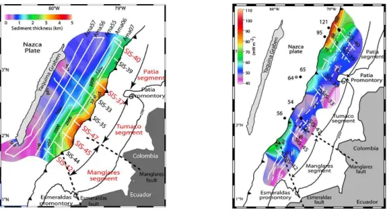
Figure 3.2.1.3-1 Segmentation of northern margin: sediment thickness and flow heat. 50 Figure 3.2.1.3-2 Segmentation of northern margin: isotherms along the subduction interface. ... 50
Figure 3.2.1.3-3 Seismic line in the Gulf of Guayaquil. ... 52
Figure 3.2.1.4-1 Cross-sections with instrumental seismicity (local catalog). ... 53
Figure 3.2.1.4-2 Cross-sections with instrumental seismicity (seismic campaigns). ... 54
Figure 3.2.2.1-1 Morphology of the continental shelf. ... 55
Figure 3.2.2.1-2 Pre-Stack-Depth Migration profile SIS05. ... 56
Figure 3.2.2.1-3: Structures in the upper plate in the central segment. ... 56
Figure 3.2.2.2-1: N-S Seismic profile in northern continental shelf. ... 58
Figure 3.2.2.2-2: N-S seismic profile in the central continental shelf. ... 58
Figure 3.2.2.2-3 Morphology of the top if the acoustic basement in the continental shelf. ... 59
Figure 3.2.2.3-1: Seismic line along the subduction of seamounts ... 60
Figure 3.2.2.4-1: Simple Bouguer gravity anomalies map. ... 61
Figure 3.2.2.4-2 Geologic cross-section along the Manabí Basin. ... 61
Figure 3.3.1-1 Seismic coupling along the northern Andes margin. ... 63
Figure 3.3.1-2 Distribution of the ISC in Ecuador. ... 64
Figure 3.3.2-1 Rupture areas and asperities of major historical earthquakes in Northern Ecuador. ... 65
Figure 3.3.3-1 Instrumental seismicity in Ecuador (Catalog for SSHA)... 66
Figure 3.3.3-2 Instrumental seismicity (RENSIG Catalog). ... 67
Figure 3.3.3-3 Cumulative seismic moment release... 67
Figure 3.3.3-4 Relocated instrumental seismicity from 1994 to 2007 (Font et al., 2013). ... 68
Figure 3.3.3-5 Seismicity during the 3 weeks-long spring-1998 campaign. ... 69
Figure 3.3.3-6 Seismicity related to the interplate seismogenic zone (ISZ), ESMERALDAS Campaign. ... 70
Figure 3.3.3-7 Coastal seismicity between 2009 and 2011 (ADN Project). ... 71
Figure 3.3.3-8 Up: Map with the seismicity during the SISTEUR Campaign. ... 72
Figure 3.3.3-9 Seismicity during May-Jun 2013, OSISEC and JUAN Projects. ... 72
Figure 3.4.1-1 Interpreted Pre-Stack-Depth Migration profile SIS05. ... 74
Figure 3.4.2-1 Characteristics of the continental shelf. ... 75
Figure 3.4.2-2 Uplift in the region of La Plata Island. ... 76
Figure 3.4.2-3 Reconstruction of the progressive eastward migration of a seamount in the top of Carnegie Ridge entering in subduction. ... 77
Figure 3.4.3-1 Shallow seismicity in the subduction zone of Ecuador (RENSIG and Font et al., catalogs). ... 78
Figure 3.4.3-2 GPS E-W measurement campaigns at the site MS01. ... 79
Figure 3.4.3-3 2005 Slow slip event modeling. ... 79
Figure 3.4.3-4 Continuous GPS Time series for the 2010 slow slip event. ... 80
Figure 3.4.3-5 Accompanying seismicity for the slow slip event of 2010. ... 80
Figure 3.4.3-6 Slip modeling for the 2010 slow slip event. ... 81
Figure 3.4.3-7 Slip modeling for the 2010 slow slip and slip deficit. ... 82
Figure 4.1.2-1 Normalized cumulative number of events in the shallow subduction zone of Ecuador... 85
Figure 4.1.2-2 Local instrumental seismicity from 1993 to present (RENSIG Catalog). ... 88
Figure 4.1.3-1 Seismicity vs. Time in the Manta-Puerto Lopez sector seen by the local permanent network (RENSIG Catalog). ... 89
Figure 4.1.4-1 Seismicity seen by the worldwide network. ... 91
Figure 4.1.4-2 Focal mechanisms of the ISZ zone. ... 92
Figure 4.2-1 Map with the OSISEC-Project stations and identified events in each station. ... 93
Figure 4.2-2 Data availability. ... 94
Figure 4.3.1-1 Clock derive for RENSIG-ADN stations... 95
Figure 4.3.1-2 Clock derive for OBS. ... 96
Figure 4.3.3-1 DEPNET Program © Régnier. ... 99
Figure 4.3.4.2-1 Space search of the best solution in the location of an earthquake. .. 100
Figure 4.3.4.3-1 Preliminary locations. ... 101
Figure 4.3.4.5-1 Comparison of earthquake’s location errors using different distribution of perturbed arrival times. ... 103
Figure 4.3.4.5-2 Comparison of number of events before and after the quality selection. ... 104
Figure 4.3.4.5-3 Distribution of earthquakes according to their quality location. ... 105
Figure 4.3.4.5-4 Quality E events. ... 106
Figure 4.3.5.1-1 Principle of the magnitude concept. ... 107
Figure 4.3.5.2-1 Characteristics of common events form the magnitude determination. ... 110
Figure 4.3.5.2-2 Amplitude vs mag. of selected events for magnitude determination. 111 Figure 4.3.5.2-3 Individual magnitude determination for the common events. ... 112
Figure 4.3.5.2-4 Results of magnitude determination for the common events. ... 113
Figure 4.3.5.2-5: Distribution of magnitudes for the initial and final catalogs. ... 114
Figure 4.3.5.3-1 Frequency-magnitude relationship. ... 115
Figure 1. Geodynamic framework of Ecuador. ... 120
Figure 2. Preliminary locations, velocity model used and depth distribution. ... 122
Figure 3. Search of velocity models, initial and final depth and rms distributions for the events in the two domains. ... 124
Figure 4. Final catalog with earthquake location quality and focal mechanisms. ... 128
Figure 5. Depth distribution in the final catalog and characteristics of focal mechanisms used to determine the top of the slab ... 131
Figure 6. Cross-sections used to determine the top of the slab. ... 133
Figure 7. Seismic segmentation, seismic coupling and geologic frame in the study region. ... 134
Figure 8. Comparison between theoretical and observed arrival times for two clustered events in the offshore region. ... 136
Figure 9. Model explaining the observed seismicity. ... 140
Figure 1A. Quality criteria for focal mechanisms. Numbers correspond to Table 2A. 149 Figure 6.1-1 Normalized cumulative number of events in the marine forearc and in the Coastal Range. ... 151
Figure 6.1-2 Seismic activity in the marine forearc during the 20-month period analyzed. ... 152
Figure 6.1-3 Seismicity in the marine forearc. ... 153
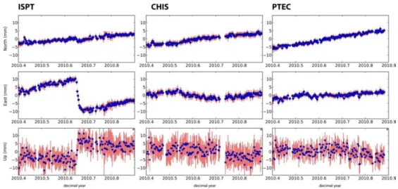
Figure 6.1-4 ISPT GPS time series from January 2012 to December 2013. ... 154
Figure 6.2-1 GPS stations analyzed and used for the kinematic model of the slow slip.
... 156
Figure 6.2-2 Daily average of GPS time series from November 24th, 2012 to February 24th, 2013. ... 157
Figure 6.2-3 Cumulative slip in the two stages of the slow slip event of 2012-2013. . 158
Figure 6.3-1 Modeled cumulative slip and the accompanying seismicity. ... 159
Figure 6.3-2 Magnitude, cumulative number of events and cumulative seismic moment during the intense phase of the seismicity ... 160
Figure 6.3-3 Daily seismicity and GPS daily averaged observations... 161
Figure 6.3-4 Snapshots of daily seismicity, modeled slip, GPS vectors (observed and modeled) and GPS time series between January 15 and 22. ... 162
Figure 6.3.1-1 Time and spatial distribution of the seismicity. ... 167
Figure 6.3.2-1 Seismicity from the end of November 2012 to April 30th 2013. ... 168
Figure 6.3.2-2 Daily number of events from the end of November 2012 to April 30th 2013. ... 169
Figure 6.3.3-1A Epicentral distribution of the families identified and waveform pattern. ... 170
Figure 6.3.3-1B Occurrence and number of events in each identified family... 171
Figure 6.3.3-1C Waveforms of the families with the largest number of members (>=3). ... 172
Figure 6.3.3-1C continued. ... 173
Figure 6.3.3-2 Magnitude range of the events in each family ... 174
Figure 6.3.4-1 Up: Seismicity and mode of faulting during de slow slip. ... 176
Figure 6.4-1 Map and normalized cumulative number of events in the Coastal Range. ... 178
Figure 6.4-2 Seismicity in the Coastal Range region (green ellipse) during the two episodes of slow slip. ... 179
Figure 6.4-3 Map view of the extension of clusters beneath the Coastal Range. Possible control of Nazca Plate structures? ... 179
Figure 6.4-4 Diagrams showing tentative scenarios to explain the change in the seismicity rate beneath the Coastal Range based on slab stresses. ... 181
Figure 6.5-1A Locations and occurrence of identified families during the observation period. ... 182
Figure 6.5-1B Waveforms of the families of events occurring mainly out of the January 2013 slow slip. ... 183
Figure 6.5-1B Waveforms of the families of events occurring mainly out of the January 2013 slow slip (continued). ... 184
Figure 6.5-1B Waveforms of the families of events occurring mainly out of the January 2013 slow slip (continued) ... 185
Figure 6.6-2 Accumulated Coulomb stress after each of the transient slips in the Figure 6.3.5-1 (Liu and Rice, 2007)... 187 Figure 6.6-3 Daily number of events and modeled aseismic moment release (colors are as in Figure 6.6-1). ... 188 Figure 6.6-4 Daily seismicity and maximum modeled amount of slip in the two patches. ... 188 Figure 6.6-5 Schema of slip patches in map view and in section view. ... 189 Figure 6.6-6 Schematic diagrams showing the daily displacement and the distribution of the seismicity. ... 189 Figure 6.6-7 Schematic diagrams in map and section views to show the onset of the seismicity in cluster 2. ... 190 Figure 7.1-1 Comparison in map view between the seismicity and the rates of tectonic deformation in the continental shelf. ... 195 Figure 7.1-2 Cross-section SIS-4 with the seismicity and the location of the subducted seamount. ... 195
1.
General
introduction
and
overview of the thesis
1.1 Importance of the study of subduction zone
earthquakes
Earthquakes in subduction zones are among the most devastating events affecting large regions and populations. The effects of large and great earthquakes in general, are not only restricted directly to the motion associated to seismic waves but also to triggered phenomena like landslides and tsunamis. The first two phenomena have a local impact, while the second may have also a regional or even global impact.
According to the observations and studies, the occurrence of large earthquakes seems to obey to a rough periodicity. This property is explained by the general model of elastic rebound proposed by Reid (1910) which has been best quantified and modeled with GPS observations in the last two decades. In this model, the earthquakes follow a cycle with a period of strain accumulation (interseismic period), then the accumulated energy is suddenly released during the earthquake (co-seismic period) and then a period of slow relaxing and readjustment (post-seismic period) and finally a new interseismic period of slow re-loading of the strain.
This cycle, simple and apparently constant in time is not really observed in the nature. Furthermore, this picture has become more complex with the discovery of a new kind of silent and slow earthquakes; silent in the sense that they do not release seismic waves as usual earthquakes do and slow because they last for several days, months or even years. They are often associated with non-volcanic tremor but occasionally with swarms of small earthquakes.
As these slow slip events likely release a considerable amount of the accumulated strain, understanding their role in the seismic cycle and the physical properties which are controlling their occurrence, is of vital importance for a correct assessment of the seismic hazard along the segments of the subduction zones where this type of events has been identified.
1.2 What does happen at the subduction zone of
Ecuador?
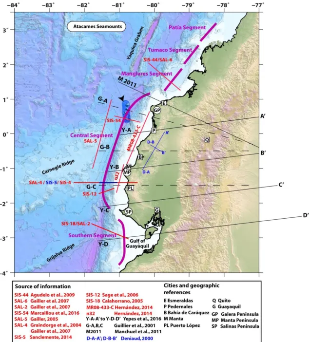
The Ecuadorian subduction zone shows a clear segmentation in its seismic behavior. The central-north region was affected by several large and great subduction earthquakes since the beginning of the XXth century, the latest being the 2016 7.8 Mw Pedernales Earthquake, while in the central-south regions no large earthquakes are known. This
segmentation seems to be related broadly with the subduction of the Carnegie Ridge which in turn has an impact on the interseismic coupling.
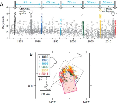
The microseismicity reveals also this segmentation. It is organized in seismic swarms, which roughly delimit the rupture areas of large earthquakes or highly coupled zones. In the central region, in front of the Carnegie Ridge, the seismic swarms are less well constrained but they extend in a wider region downdip of the highly locked zone. The seismic swarms in the central region have been the longest in duration and the largest in magnitude content.
With the recent geodetic networks deployed along the coast, slow slip events have been detected in both regions. These slow slips are also accompanied by seismic swarms, then the natural question is: were the past seismic swarms also related to slow slip events? In that sense, some studies have been developed and others are on the way. One of the most interesting results about this issue is about one of the largest and longest seismic swarm in the central zone, in 2005, which in fact has been determined to be accompanied with a slow slip with an equivalent magnitude of Mw 7.2-7.3, which is among the largest worldwide (Mw 7.5).
1.3 Main issue to be addressed
One of the main questions to be addressed about the central subduction zone of Ecuador is why did no large earthquakes occur here? If large earthquakes are associated to highly coupled asperities, why the asperity located beneath La Plata Island did not fail as the northern asperities? We probably will not have the answer because many parameters are involved and their interrelations have demonstrated to be complex and not so easy to generalize. Instead we can try to characterize the seismic behavior of this region through the deployment of a dense onshore-offshore seismic network that encompasses adequately the asperity.
The main objective of this temporal seismic network is to characterize the background seismicity, increasing the detection level and computing reliable locations, in order to document possible variations in the seismicity rate, occurrence of seismic swarms, mainshock-aftershock sequences, downdip seismicity shift, synchronous updip-downdip seismicity, etc. that may announce the occurrence or trigger new slow slip events. In short, we aim to find patterns in the seismicity that could help us to anticipate and better understand the role of the slow slip events in the seismic cycle.
1.4 Thesis outline
In Chapter 2, the reader will be provided with some concepts about stick-slip and creep phenomena along faults. Then we describe the characteristics of the subduction seismogenic zones, the factors that control their geometry, extension and behavior. Finally we describe the transient deformations in the subduction zones, principally the
slow slip events, their location, their periodicity, associated events and their role in the seismic cycle.
In Chapter 3, we present the Ecuadorian subduction zone describing the kinematics and the geological evolution of the Nazca Plate and of the forearc region of the overriding plate. We describe the shallow properties of the seismogenic zone, including the overriding plate and the subducted plate derived from active seismic data, and focus on the region of the La Plata highly-coupled patch.
Chapter 4 is devoted to the description of the seismic data used and all the chain of analysis performed to achieve our objective to characterize the background seismicity.
Chapter 5 is an article, ready to be submitted, which presents the background seismicity and a model to explain its behavior.
In Chapter 6 we present the analysis of the 2012-2013 slow slip event registered in La Plata Island region. We compare the evolution of this event with the seismicity in order to define the cause-effect relationship.
Finally Chapter 7 includes a general discussion, with comparison with other regions of the world were similar slow slip event have been observed and the major conclusions of this study.
2. The seismogenic subduction
zones
In this chapter, we present some concepts about the factors that control the brittle fracture and the aseismic creep in general. Then we focus on the phenomenology of the earthquakes in the subduction zones emphasizing on the slow slip events.
2.1 Introduction
Subduction zones are where two tectonic plates collide and one of them underthrusts the other, liberating ~90% of the seismic energy release worldwide through great and mega earthquakes (Pacheco and Sykes, 1992).
Understanding the deformation mode and seismogenic processes at this kind of limit between two plates remains crucial to contribute to hazard assessment.
In subduction zones, the slip along the interface contact zone (thrust motion) accommodates the relative convergence between the subducting and overriding plates. From the surface to intermediate depths, the interface contact zone separates elastic material on either side and at these depths the slip mode is mainly influenced by pressure, temperature and rheology, conditions that control the frictional state of the fault.
Regarding the frictional state of the fault, the slip mode can be: (i) continuous and stable; (ii) episodic in time, fast and short; (iii) episodic in time, slow and longer (Peng and Gomberg, 2010).
In the first case, the fault slides continuously. The slip mode is stable (continuous in time) and creeping. The subducting plate freely under thrusts the overriding plate without accumulating strain. In this type of contact zone, no large earthquakes can nucleate.
In the second case, the thrust fault (or part of it) shows a frictional behavior. The relative movement is locally, partially or totally blocked, inducing stresses within both plates and in the contact zone. The stress will accumulate until it exceeds the strength of the material around (friction threshold). At that moment, a sudden and fast slip liberates the accumulated strain through the radiation of seismic energy. This behavior, known as stick slip, corresponds to the one that produces earthquakes, being the earthquake the “slip” and the “stick” the period of elastic strain accumulation which corresponds to the interseismic period.
In the third case, slow slip with longer duration occurs, often episodically, with signals of lower frequency content (e.g. non volcanic tremor) and no seismic radiation. The slip
mode is limited in magnitude and occurs essentially on the downdip transition between locked (or partially locked) and stable sliding regions on the interface contact zone.
With the improvement of the instrumentation in the last decades, more information has emerged on the slip behavior in the subduction zones showing that the three slip modes can be adjacent and that they most probably interact by stress transfer (Lay and Schwartz, 2004).
2.2 Earthquakes in the subduction context
In this section, we introduce concepts on the slip behavior on the interface of subduction zones.
We first give general notions about the stick-slip model and some notions about earthquakes. We then present general characteristics of the interplate seismogenic zone.
2.2.1 Stick-slip concept
The standard model of friction from rock friction experiments states that the sliding of a block begins when the ratio of shear () to normal () stress acting over a block (Figure 2.2.1-1) reaches a value named static friction coefficient s. Once the motion initiates the sliding resistance coefficient falls to a lower value, the dynamic friction coefficient d which depends on the stiffness of the system (K) (Figure 2.2.1-1; Scholz, 1998).
Figure 2.2.1-1 Block-slider model and forces acting on the block.
When a force acts through a spring with a stiffness K, is the normal force acting on the block a kind of resistance force opposite to the sliding of the block (Scholz, 1998).
After more rock friction experiments, this behavior has been shown to be more complex, with s and d changing in their values as a function of the velocity and time involving the surface of contact during the motion. This is the rate/state-variable constitutive law that describes the rock friction shown in equation (e2.2.1-1) (Scholz, 1998). 𝜏 = [𝜇0+ 𝑎 ∗ ln(𝑉𝑉 0) + 𝑏 ∗ ln( 𝑉0∗𝜃 𝐿 )] ∗ 𝜎̅ (e2.2.1-1) Where: : Shear stress
𝜎:̅ Effective normal stress (applied normal stress – pore pressure) V: Slip velocity
V0: Reference velocity
0: Steady-state friction at V=V0
a & b: Material properties
L: Critical slip distance
: State variable which evolves according to: 𝑑𝜃𝑑𝑡 = 1 −𝜃∗𝑉𝐿 (e2.2.1-2)
Once the block is moving at a constant velocity (steady state), the shear stress is:
𝜏 = (𝜇0+ (𝑎 − 𝑏) ∗ ln𝑉𝑉
0) ∗ 𝜎̅ (e2.2.1-3)
From (e2.2.1-3), if dynamic friction d is defined as steady-state friction at velocity V, then:
𝑑𝜇𝑑
𝑑(ln 𝑉)= 𝑎 − 𝑏 (e2.2.1-4)
And if static frictions s is defined as the starting friction following a period of time t in stationary contact, then for a long t:
𝑑𝜇𝑠
𝑑(ln 𝑡)= 𝑏 (e2.2.1-5)
(e2.2.1-1) is also known as slowness law, because at steady state, the state variable is proportional to slowness (1/V) like:
𝜃𝑠𝑠=𝑉𝐿 (e2.2.1-6)
L, the critical slip distance, is interpreted as the sliding distance necessary to renew the contact population to evolve to a new steady state, then ss is the average contact lifetime.
According to (e2.2.1-4) and (e2.2.1-5), the friction coefficients depend on a, b, the time of contact with the surface t, the sliding velocity V and the critical slip distance L. The (a-b) parameter, which depends on material properties play an important role in sliding stability regimes.
If a-b >= 0, s grows with the velocity (i.e. the friction augments with the velocity of the slide). In this case, the material has a velocity strengthening behavior which is known to be at stable regime (i.e. stable sliding without stress accumulation).
Earthquakes do not originate in this regime and any motion coming from neighbor regions will be rapidly stopped due to a negative stress drop.
If a-b < 0, s drops with velocity. The material at the surface contact has a velocity weakening behavior since the friction diminishes with the velocity. Depending on a critical value of effective normal stress 𝜎̅𝑐 there are two behaviors: (i) if 𝜎̅ > 𝜎̅𝑐,sliding is unstable under quasi-static loading (constant regime); (ii) if 𝜎̅ < 𝜎̅𝑐sliding is conditionally stable under dynamic loading but can change to unstable under abrupt changes in the velocity of sliding.
For example, in the nature, the (a-b) parameter becomes positive for a crystalline crust (granite) when T>300°C. This implies that there would not be earthquakes at temperatures greater than 300°C (high P and T) (Figure 2.2.1-2). At shallower depths (lower P and T) the presence of a fault gouge (granite powder) makes (a-b) more positive because of dilatancy; this explains why it exists a stable region near the surface of a fault and why the sliding is rapidly stopped (Scholz, 1998).
Figure 2.2.1-2 Variation of the a-b parameter.
(a-b) parameter vs T for granite and granite powder (representing fault gouge) (Scholz, 1998).
In broad lines, few parameters interact on a fault to allow the initiation of a rupture and the sliding or not on the fault.
The static friction (before initiation of sliding) is growing slowly as log t when the contact surface is under load during time. When the static friction reaches a threshold value, the slide can initiate.
The dynamic friction (once the motion is initiated) depends on the sliding velocity that in turn is controlled by the material and T. The friction evolves to a new steady state value after a critical distance L when sliding velocity varies suddenly.
Parameters such as time and rheology of the surfaces in contact that influences the normal stress are involved/imbricated in the stick-slip concept and in the initiation of the rupture.
2.2.2 The subduction seismogenic zone, general concepts
In a subduction zone, the geometry of the contact zone between the two tectonic plates extends from the surface down to greater depth, involving a large range of P and T.The interplate contact zone is characterized by three stability regimes, from surface to depth: stable, unstable and finally stable again. The transition from one regime to the other is not sharp but progressive, involving regions with a conditionally stable regime (Figure 2.2.2-1). The seismogenic zone, where earthquakes can nucleate is characterized by an unstable regime. The rupture can propagate indefinitely into conditionally stable regions and they stop at stable regions (Scholz, 1998).
Figure 2.2.2-1 Seismic styles and variation of the friction stability parameter in a subduction zone.
Synoptic model of a subduction fault showing the variation of friction stability parameter: 𝑧 = (𝑎 − 𝑏) ∗ 𝑠̅; (𝑠̅ = 𝜎̅; 𝑒𝑓𝑓𝑒𝑐𝑡𝑖𝑣𝑒𝑛𝑜𝑟𝑚𝑎𝑙𝑠𝑡𝑟𝑒𝑠𝑠) and the seismic styles (modified from Scholz, 1998).
The extension of the seismogenic zone (W) is bounded superficially and at depth by the updip (U) and downdip (D) limits respectively, leaving a limited depth range for the nucleation of earthquakes (Figure 2.2.2-2) (Heuret et al., 2011). Outside of these limits, the relative convergence between the two plates is accommodated by creeping.
Figure 2.2.2-2 Parameters defining the seismogenic zone.
U: updid and D: downdip limits; W: along dip width of the zone and the dip angle. Ux, Dx, Uz, Dz are W coordinates based on 5% to 95% distribution distance of earthquakes from the trench and depth
Physically, the limits of the seismogenic zone are pressure, temperature and material controlled. The updip limit coincides with the isotherm of 100-150°C, where the accretionary prism meets competent rocks; at these temperatures, diagenesis and low grade metamorphism produce minerals of higher bulk rigidity (smectite to illite) (Aoki and Scholz, 2009). The downdip limit coincides with the onset of plasticity of the feldspar (the most ductile mineral of the basalt) at ~450 °C. Downdip limit may be greater as 45 km depth depending on thermal gradients (Scholz, 1998). It has been proposed that this limit coincides with the Moho of the upper plate (e.g. Kiushu – Japan, Yoshioka and Murakami, 2007), but as several subductions zones present deeper limits than the Moho of the upper plates (e.g. Sumatra; Simoes et al., 2004), Seno (2005) proposes that the stress regime at the mantle wedge not favoring serpentinization of the mantle wedge inhibits the stable sliding and hence extends in depth the seismogenic zone.
Downdip, the extension of a seismogenic zone can be increased if the involved subducted plate is colder and denser promoting the change of thermal gradients as seen in Fig. 2.2.2-3 from Gutscher (2002).
Figure 2.2.2-3 Subduction styles and thermal structure.
Effect of subduction on thermal structure of subduction zones which leads to an increment of the size of seismogenic zone (Gutscher, 2002).
Heuret et al. (2011) indicate that the extension of the seismogenic zone (W) could be correlated with several other parameters describing subduction zones like the subduction velocity (Vs), the thermal parameter (), the dip angle (), the depth of the downdip limit (Dz) and seismicity rate (), being the thermal parameter () equal to:
𝜑 = 𝐴 ∗ 𝑉𝑠 ∗ 𝑆𝑖𝑛𝜃 (e2.2.2-1)
With A=age of the plate; and the seismicity rate () the number interplate thrust events with magnitude Mw >= 5.5 normalized for a period of 100 years and for a trench length of 1000 km.
The results of this study are shown in Figure 2.2.2-4.
Figure 2.2.2-4 Empirical relations between several parameters describing subduction zones.
The extension of seismogenic zone or width (W) represented by colored lines present an inverse relation with the following parameters: subduction velocity (Vs), the thermal parameter (), seismicity rate (),
dip angle () and depth of downdip limit (Dz). While W increases from 1 to 3, the other parameters decrease from 1 to 3. See text for extended explanation (Heuret et al., 2011).
A faster plate (1 in Figure 2.2.2-4) and a cold plate (larger ), dips steeply (large ) into the mantle, presenting a narrow seismogenic zone (small W) with a deep downdip limit (large Dz) and a large number of moderate earthquakes (large ).
At the other end, a slow plate (3 in Figure 2.2.2-4) and a warm plate (smaller ), dips gently (smaller ) into the mantle, presenting a wider seismogenic zone (large W) with a shallow downdip limit (smaller Dz) and a smaller number of moderate earthquakes (smaller ).
The interplate seismogenic zone, i.e. capable of initiate large to great thrust earthquakes is then bounded in a limited range of depths that differ from one subduction zone to others.
2.2.3 Asperities, barriers and stability regimes
Within these ranges of depths limiting the seismogenic zone, many studies have shown that the slip distribution on the fault is very complex. The slip distribution was first explained in terms of barriers and asperities (e.g. Das and Aki 1977; Kanamori, 1981; 1994). Kinematically, an asperity is a region in the interplate where large slip occurs during a mainshock while the barrier stops the propagation (Kanamori, 1994). In this framework, several possibilities may occur on the interplate about the distribution and
1
2
behavior of the asperities and barriers: 1.When the contact surface is under loading during the time, the slip could occur outside the asperities in the form of creep and small earthquakes while during the seismic paroxysm, the asperities would break producing “characteristic” earthquakes. 2. The barriers remain locked until the next major sequence and they fail as asperities for this major sequence, in such case, this will be a “non characteristic” earthquake sequence. 3. Barriers and asperities may not be permanent (not associated to long term features like topographic reliefs in the plate) but instead, due to nonlinear frictional characteristics of the materials in the interface (Rice, 1991) or to a redistribution of water and pore pressure during earthquakes (Kanamori, 1994), their positions are redistributed along the interface, making the location and magnitudes of the next earthquakes difficult to anticipate.
A characteristic earthquake is an event which ruptures an entire fault segment (section of a fault bounded by strong barriers that stop the rupture). Alternatively, it can be an event from a sequence, rupturing the same area of the fault (same asperity) (Jackson and Kagan, 2011).
Bringing together above concepts about physical properties of the interface that favors or not the sliding, the asperity would be a region associated to a material with condition of velocity weakening behavior (unstable sliding frictional condition) while the surrounding barriers are associated to material with velocity strengthening behavior (stable sliding frictional condition). In more recent models, asperities and barriers are presented randomly distributed as the distribution of stable, unstable and conditionally stable domains (Figure 2.2.3-1) (Lay and Schwartz, 2004).
Figure 2.2.3-1 Schematic section of a subduction zone.
The complexity in friction and kinematics properties is the result of the nature of the subducted plate (Lay and Schwartz, 2004).
In this model, the shallowest part of the fault creeps steadily when stress is applied. Deeper, patches of velocity weakening material (asperities) could rupture seismically and the rupture could propagate to the surrounding conditionally stable patches. The neighboring stable nearby material may either stop the rupture (barrier) or may slide and propagate the rupture resulting in a “non-characteristic” earthquake.
2.2.4 Earthquake size
The magnitude of an earthquake on the seismogenic zone depends in part on the stable, unstable and conditionally stable properties distribution that will govern the extension of the area capable to slip during an earthquake.
Several scales of magnitudes have been proposed, many based on amplitude measurements of the seismic signal. All of them are non-dimensional values not linked to a physical parameter of the seismic event and to a certain level they do not give anymore a real estimation of the magnitude (they saturate). The scale of magnitude describing the size of an earthquake is the moment magnitude which is tied to the seismic moment.
The seismic moment is a linear measure of the size of an earthquake. It relates the size with the slip and the affected area during the earthquake (Scholz, 1998). It depends on mean slip in the fault u and A, the area of slip during the event:
𝑀0 = 𝐺 ∗ 𝑢 ∗ 𝐴 (e2.2.4-1)
With G: shear modulus. Then the rate or velocity of moment seismic release rate of a fault or plate boundary is:
𝑀̇0 = 𝐺 ∗ 𝑣 ∗ 𝐴 (e2.2.4-2)
With v: long term slip velocity determined from the plate tectonic model or geological data and A is now the total fault area.
2.2.5 Interseismic coupling
If the extension of the surface of contact with unstable behavior (velocity weakening) is large enough, the friction on that patch can block partially or totally the relative motion between the plates along that segment, while the updip and downdip regions remain creeping. The motion can then be momentarily locked (or partially locked) allowing stress accumulation between two earthquakes (which are episodes of sliding). This locking due to the coupling between both tectonic plates during the interseismic period results in a slip deficit, i.e. the amount of slip on the contact zone is insufficient to fully accommodate plate motion.
The assessment of the coupling coefficient on the interface was first measured based on the ratio of observed to expected seismic moment release in a fault segment, i.e. the ratio of the sum of the seismic moment release of all earthquakes occurring in a fault (𝑀0̇ ) to all seismic moment accumulated in the fault due to the relative convergence 𝑆 between the plates (𝑀0̇ ): 𝑇
= 𝑀0̇𝑆
𝑀0𝑇̇ (e2.2.5-1)
may vary from 0 to 1 giving information on the stability regime of the fault or on how efficiently is released the accumulated movement on the fault. When is 1, it means that all accumulated slip has been released during earthquakes (likely big ones), so all the seismogenic zone has rupture each time; in this case, the fault can be considered seismically coupled and unstable. On the contrary, when =0, no big earthquakes have released significant seismic moment; in this case the fault is considered seismically decoupled and stable (Scholz, 1998; Scholz and Campos, 2012).
Nowadays, the GPS technology and its global use allow an accurate estimate of the interseismic coupling of the interface contact zone related to the ratio between slipping velocity on the fault during the interseismic period and the long-term plate velocity. The assessment of is based on the interseismic strain acceleration of the upper plate and is a measure of the stress accumulation (Bock and Melgar, 2016). This geodetic estimate of the seismic coupling is free of earthquake sampling problem (extension and completeness of seismic catalogs).
Interseismic coupling models that describe spatially where the fault is not moving (coupled) or moving (decoupled) are constructed from strain rates transmitted into the crust and detected at the surface (e.g. Savage, 1983; McCaffrey et al., 2000; Mazzotti et al., 2000; Norabuena et al., 2004). In function of the density and coverage of the instrumentation, this estimation may be very detailed. Those models can particularly well define the downdip limit of the coupled zone, but not its upper limit due to the poor coverage or lack of GPS in the marine area where the updip limit of the seismogenic zone is projected (e.g., McCaffrey, 2002; Wang and Dixon, 2004] (Wallace et al., 2009).
According to Scholz and Campos (2012), high seismic coupling occurs for subduction zones subjected to high normal forces. Normal stresses loading the interface may come from the subduction of topographic features like seamounts (e.g. Scholz and Small, 1997), they may come from the weight of the overlying crust (Tassara, 2010), or from the tectonic stress state and structural permeability of the overriding plate that allows higher or lower fluid pressures along the interface (Wallace et al., 2012). Furthermore, earthquake asperities correlate with areas of high coupling. Seismic coupling has therefore a semblance of permanence (persistency) and it may be well assessed through discrete movements along the interface (earthquakes).
Comparing to classical definition and assessment of seismic coupling, interseismic coupling carries a dynamic or changing connotation and accurately reflects more complex phenomena in the interface zone. For example, several detailed studies using seismicity observations show how interseismic coupling changes in a region from strong coupled to weak coupled before large earthquakes which is interpreted as a gradual unlocking of the interface contact zone (e.g. before Iquique 8.1 Mw, 2014 earthquake, Schurr et al., 2014; Kato et al., 2016).
2.2.5.1 The effect of subducted topographic features in the seismic coupling
Topographic features such as horst and grabens, submarine volcanoes, isolated or multi-peaks seamounts, ridges, fossil or active rifts, plateaus and volcanic arcs are all called “asperities”. The main effect of these asperities when they are incorporated in the subduction process is to strongly increase the tectonic erosion in the interface contact zone and to generate multiple deformations on the overriding plate. Among the effects in the overriding plate are the multiple events of vertical movements along the margin (uplift and subsidence) (Lallemand, 1999).
In the framework of the present work, we are interested in the effect of the subduction of seamounts and ridges on the seismic coupling and hence in the generation of large earthquakes.
In one hand, the seamounts and ridges are positive features in the oceanic floor presenting large resistance to the subduction. For this reason, they have been considered as “strong asperities” which increase the seismic coupling (e.g. Cloos, 1992; Scholz and Small, 1997), but few M>6.5 events have been linked to seamounts (Wang and Bilek, 2011). According to Yang et al. (2012) the seamount as a patch of elevated normal stress on the interface can fail or impede a megathrust earthquake in function of its position to the earthquake nucleation (when it sits at the updip or downdip regions of the seismogenic zone, the seamount has little effect; if it is at intermediate distance range up-dip of the nucleation zone, the seamount can inhibit or nucleate earthquake ruptures depending on the stress conditions).
In the other hand, the subduction of positive relief creates a volume of damage developing a network of fractures where large earthquakes cannot nucleate and conversely, small earthquakes and aseismic creep are common (Wang and Bilek, 2011).
2.2.6 The seismic cycle
From the persistency of the coupled patches along the interface contact zone and the continuity of the relative convergence derives the notion of seismic cycle
The seismic cycle is defined as the time elapsed between two major earthquakes in the same fault segment.
Between two events, during the interseismic period, the stress builds up while the contact zone and their surroundings accumulate strain. During that period of time (several decades or hundreds of years) the overriding lithosphere shows shortening and uplift.
When the strength of the elastic material is exceeded by the accumulated strain, the earthquake occurs, releasing in a few seconds/minutes the accumulated strain through the thrust motion on the fault. The upper lithosphere relaxes and shows extension and a consequent subsidence and some uplift near the trench (Figure 2.2.6-1).
During the postseismic period (minutes, decades to months) both, the fault and the crustal material adjust the stresses and the strain imposed by the earthquake. Additional slip (after slip) can occur along the fault with further extra flow in the lower crust (visco-elastic relaxation).
The recurrence time interval between two mainshocks is not constant. Even the buildup of strain occurs at a constant rate, physical and/or rheological controlling the stress accumulation and the failure threshold may affect the expected cyclicity of this process (Mc Guire, 2008; Hyndman and Rogers, 2010) (Figure 2.2.6-2).
Figure 2.2.6-1 The seismic cycle.
Schematic representation of the seismic cycle in a cross-section of a subduction representing the strain buildup and release along the interface contact zone and the parallel phenomena in the overriding plate