Diversity in the tail of the intersecting brane landscape
The MIT Faculty has made this article openly available.
Please share
how this access benefits you. Your story matters.
Citation
Rosenhaus, Vladimir, and Washington Taylor. “Diversity in the Tail of
the Intersecting Brane Landscape.” Journal of High Energy Physics
2009, no. 06 (June 1, 2009): 073–073.
As Published
http://dx.doi.org/10.1088/1126-6708/2009/06/073
Publisher
Springer-Verlag
Version
Original manuscript
Citable link
http://hdl.handle.net/1721.1/88564
Terms of Use
Creative Commons Attribution-Noncommercial-Share Alike
Preprint typeset in JHEP style - HYPER VERSION MIT-CTP-4033
Diversity in the Tail
of the Intersecting Brane Landscape
Vladimir Rosenhaus and Washington Taylor
Center for Theoretical Physics MIT
Cambridge, MA 02139, USA vladr, wati at mit.edu
Abstract: Techniques are developed for exploring the complete space of intersecting brane models on an orientifold. The classification of all solutions for the widely-studied T6/Z2×Z2
orientifold is made possible by computing all combinations of branes with negative tadpole contributions. This provides the necessary information to systematically and efficiently identify all models in this class with specific characteristics. In particular, all ways in which a desired group G can be realized by a system of intersecting branes can be enumerated in polynomial time. We identify all distinct brane realizations of the gauge groups SU (3) × SU (2) and SU (3)×SU (2)×U (1) which can be embedded in any model which is compatible with the tadpole and SUSY constraints. We compute the distribution of the number of generations of “quarks” and find that 3 is neither suppressed nor particularly enhanced compared to other odd generation numbers. The overall distribution of models is found to have a long tail. Despite disproportionate suppression of models in the tail by K-theory constraints, the tail of the distribution contains much of the diversity of low-energy physics structure.
Contents
1. Introduction 1
2. Review of Intersecting Brane Models 4
2.1 General IBM’s 4
2.2 T6/Z2× Z2 4
2.3 The space of SUSY IBM models 9
3. Constructing A-brane configurations 10
3.1 Bounds from SUSY and Tadpole Constraints 11
3.2 Algorithm 14
3.3 Results 17
4. Models containing gauge group G 20
4.1 Systematic construction of brane realizations of G 21
4.2 Realizations of SU (N ) 23
4.3 Realizations of SU (3) × SU (2) 26
4.3.1 Enumeration of distinct realizations for SU (3) × SU (2) 26
4.3.2 Gauge group SU (3) × SU (2) × U (1) 28
4.3.3 Tilted tori 28
4.3.4 Distribution of generation numbers 30
4.4 Realizations of SU (N ) × SU (2) × SU (2) 32
4.5 K-theory constraints 32
4.6 Comparison with previous results on IBM model-building 34
4.7 Other toroidal orbifolds 36
5. Diversity in the “tail” of the IBM distribution 37
6. Conclusions 41
A. Appendix 43
1. Introduction
Intersecting Brane Models [1] have been studied for many years as a simple class of string theory constructions giving rise to low-energy physics theories containing a number of de-sirable features. In particular, these models give rise to low-energy 4-dimensional gauge theories with chiral fermions [2,3], and have been shown to include supersymmetric mod-els with quasi-realistic phenomenology. For reviews of the subject of intersecting brane
models, see [4,5,6,7,8,9,10]. Recently, much work has been done on understanding non-perturbative instanton effects in these models, which are relevant for computing Yukawa couplings and for supersymmetry breaking. These developments are reviewed in [11]
In this paper we carry out a detailed analysis of a well-studied class of string com-pactifications, namely intersecting brane models on the toroidal T6/Z2 × Z2 orientifold
[12]. These models are computationally very simple, and have been explored extensively. Supersymmetric models have been found in this class with 3 generations of matter in a standard model-like structure [13,14,15,16,17,18].
The mathematical structure of the vacuum classification problem for intersecting brane models is similar in many ways to that of other string vacuum constructions, such as flux compactifications in type IIB string theory. In all these cases, supersymmetry conditions imply a positive-definite constraint on the topological degrees of freedom encoding the vacuum configuration (i.e. brane windings or fluxes). Topological constraints give a limit to the total tadpole contribution from these combinatorial degrees of freedom, so that the mathematical problem of classifying vacua becomes one of solving a partition problem.
For the intersecting brane models we consider here, this partition problem is compli-cated by the fact that configurations are allowed in which some tadpoles become negative. These branes with negative tadpoles make even a proof of finiteness of vacuum solutions rather nontrivial. Early work on IBM’s on the T6/Z2 × Z2 orientifold focused on
solu-tions with certain physical properties. Some systematic analysis of models looking for solutions with standard model-like properties was done in [18]. A systematic computer search through the space of all solutions was carried out in [19, 20]. In some 45 years of computer time (using clusters), 1.66 ×10⁸consistent models were identified. The results of this analysis suggested that the gauge group and number of generations of various matter fields were essentially independently and fairly broadly distributed, without constraints (up to some upper bounds) in the space of available models, and estimates were given for the frequency of occurrence of various physical features in the models. In [21], the role of branes with negative tadpole contributions (“A-branes”)1 was systematically analyzed. It was proven there that the total number of supersymmetric IBM vacuum solutions in this model is finite. Further evidence was given for the broad and independent distributions of gauge group components and numbers of matter fields. Furthermore, analytic tools and estimates were given for numbers of brane configurations with certain properties.
In this paper we complete the program of analysis begun in [21]. We systematically analyze the possible configurations of negative-tadpole A-branes which can arise in models of this type. We develop polynomial time algorithms for classifying all A-brane config-urations, and numerically determine that there are precisely 99,479 such configurations satisfying supersymmetry and tadpole constraints. For each of these A-brane configura-tions, the distribution of remaining branes is given by a partition problem with all branes contributing positive amounts to all tadpoles, so the complete range of models with any de-sired properties can be carried out in a straightforward fashion given the data on A-brane combinations.
1Such branes were referred to as “NZ” branes in [18], and “type IV” branes in [28]; we will follow the
The analysis in this paper is a prototype for other classes of models, such as magnetized brane models on Calabi-Yau manifolds, which may present similar challenges for analyzing vacua due to negative tadpole contributions. The results on A-brane configurations enable us to systematically analyze all IBM models on the orbifold of interest with specific physical features. In particular, it is possible to efficiently classify all ways in which a particular gauge group G can appear as a subgroup of the full gauge group. We carry out this analysis for the gauge subgroup G = SU(3) × SU(2), and find some 218,379 distinct ways in which this group G can be realized as a subgroup of the gauge group while satisfying SUSY and undersaturating the tadpole constraints. These constructions can be extended to some 16 million distinct realizations of SU (3) × SU (2) × U (1), which we have also enumerated. We look at the number of generations of “quarks” in the (3, 2) representation of the gauge group, and find that this generation number generally ranges from 1 to about O(10), is peaked at 1 and ranges out to 100 or so, with no particular suppression or enhancement of 3 generations relative to other odd generation numbers. In principle all of these constructions of gauge groups of interest can be extended to all complete models containing each realization. K-theory constraints then substantially reduce the number of total possible models.
It is interesting to compare the results of our analysis with those of Gmeiner, Blu-menhagen, Honecker, L¨ust and Weigand [20]. Those authors carried out a computer scan through models by looking at configurations with small values of toroidal moduli (converted to integers). Their program generated a large class of models arising from constructing all possible combinations of the set of branes compatible with each fixed set of small moduli. While there are many more models for a typical set of small moduli than a typical set of large moduli, we find that the full distribution of models has a very long tail. There are many configurations, particularly those with one or more A-branes, which have large values of the (integer-converted) moduli. For these larger moduli, the number of combina-torial possibilities for models is smaller than for small moduli. Nonetheless, there are many distinct moduli for which some models are possible, and the configurations of branes in the tail have a wider range of variability. For example, most of the SU(3) × SU(2) models we have found lie outside the range of moduli scanned in [20]. The long tail of the distri-bution and the increased diversity of configurations in the tail explain how it is that the computer search by Gmeiner et al. may have covered the region of moduli space containing the greatest total number of models, and nonetheless did not encounter over 95% of the possible ways in which an SU(3) × SU(2) × U(1) gauge subgroup can be constructed. In general, we expect the wider diversity of models in the tail to lead to a greater probabil-ity of generating models with properties of specific physical interest. So, the answer to a question about “generic” properties of a typical model will depend crucially on how the question is posed. For example if we sample all IBM models which saturate the tadpole conditions and ask for generic properties of random models with given gauge subgroup G, we may get a very different answer than if we sample all distinct ways in which the gauge subgroup G can be realized, independent of the number of other components which can be included in the gauge group through extra branes. Our results suggest in particular that models with a desired gauge group and specific other features (like a particular generation
number, no chiral exotic fields, etc.) may be more likely to be found in the “tail” of the distribution than in the “bulk”.
The structure of this paper is as follows. In Section 2 we review earlier work on intersecting brane models on the toroidal orientifold of interest and define terminology and notation needed for the analysis of the rest of the paper. Section 3 contains a complete analysis of the range of possible A-brane configurations. In Section4we demonstrate how all configurations realizing a desired gauge subgroup G can be enumerated in polynomial time, and give the results of such an enumeration for G = SU(3) × SU(2) and SU (3) × SU (2) × U (1). Section 5 contains a comparison of our results with those of the moduli-based search of [20], and a discussion of the “tail” of the vacuum distribution. We conclude in Section6 with a summary and discussion of further related questions.
2. Review of Intersecting Brane Models
The general structure of intersecting brane models is reviewed in, for example, [7]. We briefly review some of the basic structure of these models relevant for this paper. For the most part we follow the notation and conventions of [7,21].
2.1 General IBM’s
Intersecting brane models are constructed by considering a string compactification on some Calabi-Yau manifold, including branes which can be wrapped around topologically non-trivial cycles in the manifold. The situation of interest here involves supersymmetric con-figurations of D6-branes wrapped on supersymmetric (special Lagrangian) three-cycles on the Calabi-Yau. Such brane configurations arise when type IIA string theory is compacti-fied on a Calabi-Yau with an orientifold six-plane (O6-plane); the D6-branes are needed in this situation to cancel the negative Ramond-Ramond charge carried by the O6-plane. At points where the branes intersect, there are massless string states giving chiral fermions in the four-dimensional low-energy theory in the uncompactified directions [3].
2.2 T6/Z 2× Z2
The specific class of models which we analyze in this paper arise from an orientifold on a particular orbifold limit of a Yau. Situations where a singular limit of a Calabi-Yau can be described as a toroidal orbifold are particularly easy to analyze and have long been used as the simplest examples of string compactifications with given amounts of supersymmetry. In this case we consider the toroidal orbifold T6/Z
2× Z2. Considering the
T6 as a product of three 2-tori with complex coordinates zi, i = 1, 2, 3, the orbifold group
is generated by the actions
ρ1: (z1, z2, z3) → (−z1, −z2, z3), ρ2: (z1, z2, z3) → (−z1, z2, −z3). (2.1)
The product of these generators gives an additional element of the orbifold group ρ3 =
ρ1ρ2 : (z1, z2, z3) → (z1, −z2, −z3). The geometric part of the orientifold action is given by
The symmetry of the T6 under the orbifold and orientifold actions fixes many of the moduli parameterizing the shape of the torus. Symmetry under the orbifold group guarantees that the torus factorizes as a product of three 2-tori. Symmetry under the orientifold action constrains the complex structure of each torus. For each torus the complex structure τ = a + ib must map to ¯τ = a − ib, which must be in the 2D lattice generated by (1, τ ), so τ + ¯τ = 2a must be in the lattice. This implies that either a = 0 or a = 1/2, so that the torus is either rectangular or tilted by one half cycle.
Wrapped branes and tadpoles
Consider first the case where T6 is the product of three rectangular 2-tori. In this case supersymmetric D6-branes associated with special Lagrangian 3-cycles on the T6which are invariant under the orbifold group can be described in terms of winding numbers (ni, mi) on the three 2-tori. A brane which cannot be decomposed into multiple copies of a brane with smaller winding numbers has (ni, mi) relatively prime for all i, and is known as a primitive brane. Each brane has an image under the orientifold action with winding numbers (ni, −mi).
There are Ramond-Ramond charges associated with the O6-plane which must be can-celled by the wrapped D6-branes for consistency of the model in the absence of other Ramond-Ramond sources (such as fluxes). Each element ρ in the orbifold group (includ-ing the identity) gives rise to an orientifold transformation Ωρ= Ωρ which, coupled with world-sheet orientifold reversal, gives a symmetry of the string theory and is associated with an orientifold charge on the fixed plane of Ωρ. This gives rise to 4 independent tadpole cancellation conditions, associated with total 6-brane charge along the directions (x1x2x3), (x1, y2, y3), (y1, x2, y3), (y1, y2, x3). Labeling these tadpoles P, Q, R, S, each brane with winding numbers (ni, mi) contributes to the tadpoles (with appropriate sign conven-tions)
P = n1n2n3 Q = −n1m2m3
R = −m1n2m3 (2.3)
S = −m1m2n3.
The cancellation of tadpoles requires that summing over all branes, indexed by a, must give X a Pa= X a Qa= X a Ra= X a Sa= T = 8 (2.4)
where −T = −8 is the contribution to each tadpole from the O6-plane. When giving explicit examples of branes we will generally indicate the brane by the values of the tadpoles, with winding numbers as subscripts, in the form
(P, Q, R, S)(n1,m1;n2,m2;n3,m3)= (−1, 1, 1, 1)(1,1;1,1;−1,−1) (2.5)
Supersymmetry imposes further conditions on the winding numbers of the branes. The three moduli associated with the shapes of the three 2-tori can be encoded in three positive parameters2 j, k, l, in terms of which the supersymmetry conditions become
m1m2m3− jm1n2n3− kn1m2n3− ln1n2m3 = 0 (2.6) and P +1 jQ + 1 kR + 1 lS > 0 (2.7)
for each brane separately, with the same positive values of the moduli j, k, l for all branes. When all tadpoles are nonvanishing, (2.6) can be rewritten as
1 P + j Q + k R + l S = 0 . (2.8)
Finally, there is a further discrete constraint from K-theory which states that when we sum over all branes we must have [22]
X a ma1ma2ma3 ≡X a ma1na2na3 ≡X a na1ma2na3 ≡X a na1na2ma3 ≡ 0 (mod 2) , (2.9)
where nai, mai give the winding numbers of the ath brane on the ith torus. As we will see, this discrete constraint significantly decreases the extreme end of the tail of the distribution of allowed models on the moduli space.
Branes on tilted tori
Now, we return to the case where the torus is tilted, with Re τ = 1/2. Say the ith torus is tilted. In this case, we can define winding numbers ˆni, ˆmiaround generating cycles
[ai], [bi] of the tilted torus3. In terms of these winding numbers, we can define
ni= ˆni, m˜i = ˆmi+
1
2nˆi (2.10)
which represent the number of times the brane winds along the perpendicular x, y axes on the ith torus. The supersymmetry conditions for a brane on a tilted torus are again (2.6, 2.7) in terms of ni, ˜mi defined in (2.10). The tadpole conditions on a tilted torus are given
by (2.4) where we use mi = 2 ˜mi on the tilted tori [28]. A difference which arises on the
tilted torus is that the range of values allowed for (ni, ˜mi) is different from the condition
of relatively prime integers imposed on the winding numbers for the rectangular torus. On the tilted torus, the winding numbers ˆni, ˆmi must be relatively prime integers. Integrality
of ˆni, ˆmi imposes the constraint that on a tilted torus we must have ni≡ 2 ˜mi(mod 2). The
relative primality constraint on ˆni, ˆmi becomes the condition that ni, 2 ˜mi have no common
prime factor p > 2, while for p = 2 we can have ni and 2 ˜mi both even iff ni/2 and ˜mi are
not congruent mod 2. Because of the common form of the tadpole relations, enumeration 2
These parameters are j = j2j3, k = j1j3, l = j1j2 in terms of the (imaginary) toroidal moduli τk= i/jk
for rectangular tori.
3Following the conventions of [7], these generating cycles are given on the complex plane by 2π(Ri 1+
iRi
of branes on tilted tori is closely related to that of branes on rectangular tori, with some minor modifications from the modified relative primality constraint.
Model construction
We can now summarize the degrees of freedom and necessary conditions on these degrees of freedom which must be satisfied to construct an intersecting brane model on T6/Z2 × Z2. First, we can have anywhere from 0-3 tilted tori, with the remaining tori rectangular. Then, we wrap any number of branes on the tori, described by winding numbers ni, mi, i = 1, 2, 3 for each brane, subject to the appropriate primitivity conditions for rectangular/tilted tori, so that the total tadpole from the branes is (2.4). The K-theory constraints (2.9) must be satisfied by the total brane configuration. Finally, moduli j, k, l must be chosen so that the supersymmetry conditions (2.6) and (2.7) are satisfied for each brane. Note that in general 3 branes will be sufficient to completely constrain the moduli, which are then rational numbers since the constraint equations are linear with rational coefficients. In some cases with fewer branes or redundant constraint equations, there are one or two remaining unfixed moduli. In these cases we can always choose representative combinations of moduli which are rational, though this choice is not unique.
Symmetries
The T6/Z2× Z2 model has a number of symmetries under which related models should
be identified. Permutations of the three tori can give arbitrary permutations on the indices i = 1, 2, 3 of the winding pairs (ni, mi), and hence the same permutation on the tadpoles
Q, R, S and moduli j, k, l. By 90 degree rotations ni → mi → −ni on two of the tori,
we have a further symmetry under exchange of P with any of the other tadpoles. This extends the symmetry to the full permutation group on the set of 4 tadpoles. (To realize this symmetry on the moduli it is convenient to write the moduli as j/h, k/h, l/h, so that h plays a symmetric role to the other moduli. When the original moduli are rational, we can then uniquely choose h, j, k, l to be integers without a common denominator. We will go back and forth freely between these two descriptions in terms of 3 rational or 4 integral moduli.)
There is a further set of symmetries on the winding numbers which do not affect the tadpoles. We can rotate two tori by 180 degrees, changing sign on ni, mi for two of the
i’s. Each brane also has an orientifold image given by negating all mi’s. We will keep only
one orientifold copy of each brane, and fix the winding number symmetries as in section 2.2 of [21] by keeping only branes with certain combinations of winding number signs, as described there.
Types of branes
There are three distinct types of branes which are compatible with the supersymmetry conditions. These types are distinguished by the numbers of nonzero tadpoles and the signs of the tadpoles. The allowed brane types are:
An example of an A-brane is
(P, Q, R, S)(n1,m1;n2,m2;n3,m3) = (−1, 1, 2, 2)(1,2;1,1;−1,−1). (2.11)
B-branes: These branes have 2 nonzero tadpoles, both positive. An example of a B-brane is
(P, Q, R, S)(n1,m1;n2,m2;n3,m3)= (1, 0, 0, 1)(1,1;1,−1;1,0). (2.12)
C-branes: These branes have only 1 nonzero tadpole, and are wrapped on cycles associated with the O6 charge. An example of a C-brane is
(P, Q, R, S)(n1,m1;n2,m2;n3,m3)= (1, 0, 0, 0)(1,0;1,0;1,0). (2.13)
C-branes are often referred to as “filler” branes in the literature, since they automatically satisfy the SUSY conditions and can be added to any configuration which undersaturates the tadpoles to fill up the total tadpole constraint.
Low-energy gauge groups and matter content
Given a set of branes and moduli satisfying the tadpole, supersymmetry, and K-theory constraints, the gauge group and matter content of the low-energy 4-dimensional field theory arising from the associated compactification of string theory can be determined from the topological structure of the branes.
A set of N identical branes of type A or B give rise to a U(N) gauge group in the low-energy theory, from the N × N strings stretching between the branes. A set of N identical type C branes, on the other hand, which are coincident with their orientifold images, give rise to a group4 Sp(N).
Associated with each pair of branes there are matter fields containing chiral fermions associated with strings stretching between the branes. These matter fields transform in the bifundamental of the two gauge groups of the branes. The number of copies (generations) of these comes from the intersection number between the branes. For two branes with winding numbers ni, mi and ˇni, ˇmi, the intersection number is
I =Y
i
(nimiˇ − ˇnimi) . (2.14)
Because of the orientifold, there is a distinction between A and B type branes a, b, which have images a06= a and b0 6= b under the action of Ω, and a C type brane c, which is taken to itself under the action of Ω. Given two A-type branes a, ˆa, for example, the intersection numbers Iaˆa and Iaˆa0 are distinct, and must be computed separately, corresponding to
matter fields in the fundamental and antifundamental representations of the gauge group on the branes ˆa. The same is true of type B branes, but not type C branes, which are equal to their orientifold images. Note that on tilted tori, in the intersection formula (2.14), the 4There are a variety of notations for symplectic groups in the math and physics literature. By Sp(N)
we denote the symplectic group of 2N × 2N matrices composing the real compact Lie group whose algebra has Cartan classification CN, which can be defined as Sp(N ) = U (2N ) ∩ Sp(2N, C). Note that this group
winding number ˜mi is used in place of mi. Note also that for branes a, d of any type the parity of Iad and Iad0 are the same, so that the sum Iad+ Iad0 is always even. This means
that if there is a stack of N branes a and 2 branes d of type A or B, the number of matter fields in the fundamental of SU (N ) and the fundamental of SU (2) (which is equivalent to the antifundamental) is even unless there is a tilted torus in at least one dimension. 2.3 The space of SUSY IBM models
As reviewed in [7], the first intersecting brane models with chiral matter which were con-structed lacked supersymmetry. There are an infinite number of such models, which gener-ally have perturbative or nonperturbative instabilities. In this paper we restrict attention to supersymmetric models, which have a more robust structure.
For the IBM models on the T6/Z2 × Z2 orientifold described above, the problem
of constructing supersymmetric models amounts to solving a partition problem. If we have a set of branes indexed by a, for each a the tadpoles form a 4-vector of integers (Pa, Qa, Ra, Sa). The tadpole constraint says that the sum of these vectors must equal
the vector (T, T, T, T ) = (8, 8, 8, 8) associated with the orientifold charges. If all tadpoles Pa, · · · , Sa were nonnegative, with each brane having at least one positive tadpole, then
the number of solutions of the associated partition problem would obviously be finite, as the number of possible tadpole charges would be at most 84− 1 = 4095, a subset of which would be described by a nonzero but finite number of winding number configurations, and the maximum total number of branes would be 32. With some branes allowed to have one negative tadpole, however, it is no longer so clear that the number of solutions of the partition problem must be finite, or even that the number of branes in any solution is bounded.
For fixed values of the moduli j, k, l, it is fairly straightforward to demonstrate that the number of solutions is finite [19]. The SUSY inequality (2.7) states that the linear combination of tadpoles γa = Pa+ Qa/j + Ra/k + Sa/l is positive for every brane. The
total of this quantity over all branes must be T (1+1/j +1/k+1/l), and is therefore bounded for fixed moduli. The contribution to γafrom each brane is bigger than any of the individual
contributions from any positive term. To see this, assume for example that Qa > 0, and
we will show that γa> Qa/j. Assume without loss of generality that Pa= −P < 0. From
the SUSY equality (2.8) we have k/Ra < 1/P , so Ra/k > P . Recalling that at most one
tadpole is negative, we then have γa> Qa/j + Ra/k − P > Qa/j. Thus, for fixed moduli,
we have bounded each individual positive tadpole contribution. But since each winding number appears in two tadpoles, this bounds all winding numbers. It follows that there are a finite number of different possible branes consistent with the SUSY conditions for fixed moduli j, k, l. There is therefore a minimum required contribution to γa, and therefore a
maximum number of branes which can be combined in any model saturating the tadpole conditions, proving that there are a finite number of models for fixed moduli.
In [19, 20], the space of solutions was scanned by systematically running through moduli and finding all solutions saturating the tadpole conditions and solving the SUSY and K-theory constraints for each combination of moduli. Writing the moduli as a 4-tuple of integers ~U = (h, j, k, l) as discussed above, they scanned all solutions up to | ~U | = 12.
This computer analysis produced some 1.66 ×10⁸ SUSY solutions. Their numerical results indicated that the number of models was decreasing fairly quickly as the norm of the moduli vector increased, so that this set of models seemed to represent the bulk of the solution space.
In [21], an analytic approach was taken to analyzing the space of SUSY models. In this paper it was demonstrated using the SUSY conditions that even including all possible moduli, the total number of brane configurations giving SUSY models saturating the tad-pole condition is finite. Estimates were found for numbers of models with particular brane structure.
In this paper we complete this analysis. The key to constructing all models with some desired structure is to deal with the A-branes systematically. In the next section, we de-scribe how all 99,479 distinct A-brane combinations which do not over-saturate the tadpole conditions can be constructed. For each of these combinations it is then straightforward, if tedious, to construct all models which complete the tadpole conditions through addition of type B and C branes.
3. Constructing A-brane configurations
As discussed above, finding all models in which a combination of branes satisfy the SUSY and tadpole conditions for some set of moduli would be straightforward if all branes had only positive tadpoles. In this situation, all tadpoles in each brane would give positive contributions to the tadpole condition. This would give us upper bounds on the winding numbers for all the branes and on the maximum number of branes in a given configuration. This would then allow us to scan over all allowed winding numbers and hence find all possible models, or all models with some particular desired properties.
Since A-branes have a negative tadpole, however, the tadpole constraint alone will not give us upper bounds on the winding numbers. In order to obtain such upper bounds we need to use a combination of the tadpole condition and the SUSY condition. Indeed, this approach was used in [21] to prove that the total number of supersymmetric brane configurations satisfying the tadpole condition is finite. The bounds determined in that paper, however, are too coarse to allow a search for all models in any reasonable amount of time. In this section we obtain tighter bounds, and describe how these can be used to implement a systematic search for all allowed A-brane combinations. We have carried out such a search, and describe the results here.
The goal of this section is thus the construction of all possible configurations of A-branes compatible with the tadpole and SUSY constraints. Having all A-brane configura-tions is a crucial step in performing a complete search for any class of models. In 3.1 we develop analytic bounds on the various combinations of A-branes with different negative tadpoles. These bounds are derived using combinations of the tadpole and SUSY condi-tions in order to place upper bounds on the winding numbers and the maximum number of branes allowed in a configuration. Then in 3.2 we apply these bounds to construct a complete algorithm for generating all A-brane configurations. In 3.3 we summarize the results of an exhaustive numerical analysis of all the A-brane combinations. In this section
we will be working exclusively with A-type branes. In the following section we describe how to systematically add B- and C-branes to form all configurations with desired physical properties.
To simplify the discussion we define some notation. We let [p, q, r, s] denote a configura-tion consisting of p branes with a negative P tadpole, q branes with a negative Q tadpole, r branes with a negative R tadpole and s branes with a negative S tadpole. Through permutations in the ordering, we can always arrange the branes so that the branes with a negative P tadpole are first in the configuration, followed by those with a negative Q tadpole, then R, then S. Within these groupings the negative tadpoles can be canonically ordered in increasing order of magnitude. A subscript a on a tadpole (Paetc.) will indicate which brane it belongs to. Also, for convenience, in this section we will write all tadpole numbers as the absolute value of the tadpole contribution, and explicitly insert the minus sign when needed. For instance the tadpoles of a brane a ≤ p with a negative P tadpole will be written as (−Pa, Qa, Ra, Sa). In the same manner, whenever we write a winding number ni or mi, it will mean the absolute value of the winding number and we will ex-plicitly insert a minus sign when needed. Throughout this section we will work with four integer moduli h, j, k, l for symmetry in the equations. Also, as in Section 2, the tadpole bound of 8 is denoted by T .
3.1 Bounds from SUSY and Tadpole Constraints
We will classify the A-brane configurations in terms of how many different types of tadpoles are negative. There will be four cases to consider: [p, 0, 0, 0] which corresponds to only the P tadpole being negative, [p, q, 0, 0] in which the first p branes have a negative P tadpole and the next q branes have a negative Q tadpole, [p, q, r, 0], and [p, q, r, s].
We begin with the simplest case, [p, 0, 0, 0], for which we can immediately derive bounds on the winding numbers. We then derive several general conditions which are useful in proving tight bounds on the winding numbers in the cases [p, q, 0, 0] and [p, q, r, 0]. We end this subsection by finding strong bounds for the winding numbers in the case [p, q, r, s]. In fact, it turns out that there are no combinations of A-branes which include branes with each of the four tadpoles being negative, so there are in fact no allowed combinations of type [p, q, r, s] with p, q, r, s > 0. The details of the proof of this statement are given in the Appendix. This result, however, makes the analysis of all A-brane combinations much easier, since it immediately indicates that there are at most 8 A-branes in any combination (since all have positive tadpoles Sa> 0, withPiSa≤ 8).
As the simplest case, we now consider the [p, 0, 0, 0] combinations, which contain p branes with tadpoles (−Pa, Qa, Ra, Sa), 1 ≤ a ≤ p. Since the Q, R, and S tadpoles are each at least 1, and the sums of the Q, R, and S tadpoles must each be less than or equal to T , there can be a maximum of T branes per configuration. More explicitly, each brane has 6 winding numbers ni, mi from which the 4 tadpoles are constructed as cubic combinations through (2.3). Each winding number appears in 2 different tadpoles (for example, n1
appears in the P and Q tadpoles). All 6 winding numbers appear in at least one of the Q, R, or S tadpoles. Since all the negative tadpoles are P , all 6 of the winding numbers for each brane can be bounded from the tadpole constraint applied to the Q, R, and S tadpoles.
For instance, the tadpole constraint tells us that the sum of the Q tadpoles is less than or equal to T. Thus, the sum over branes of n1m2m3 is ≤ T = 8, which gives a strong upper bound on the winding numbers na1, ma2, ma3. We can easily enumerate the allowed [p, 0, 0, 0] combinations by considering all winding numbers for the first brane which give Q1, R1, S1 ≤ T , then constructing all second branes which give Q1+ Q2 ≤ T, . . ., and so on up to at most T = 8 branes.
The other cases, with more than one type of negative tadpole, require a somewhat more complicated analysis. In the case [p, 0, 0, 0] we did not need to use the SUSY conditions. In the cases where there is more than one different negative tadpole, however, it is not immediately clear how to bound the number of branes in a configuration. The SUSY condition will play an essential role in this constraint. Rather than immediately analyzing the next case, where both P and Q tadpoles can be negative, we will find it useful to first derive several conditions which will be helpful to us for bounding the winding numbers and number of branes in a general configuration.
In the first condition that we derive we consider the subset of branes in the configu-ration with negative P or Q tadpoles (i.e., the first p + q branes). Among the first p + q branes in any A-brane configuration (ordered as described above) there are no negative R or S tadpoles. When considering constructions of the type [p, q, 0, 0] we can therefore use the tadpole constraints for the R and S tadpoles to bound 5 of the 6 winding numbers. n1 is the only winding number which is not immediately bounded by the tadpole conditions, since it is the only one that does not appear in the R or S tadpoles. We now determine a bound for these n1 winding numbers.
First Winding Number Bound (FWNB)
Again, we consider the first p + q branes, which are those having only negative P or Q tadpoles. We choose a, b from a ∈ {1, ..., p}, b ∈ {p + 1, ...p + q}. The SUSY condition (2.8) for brane a states −Ph
a + j Qa + k Ra + l
Sa = 0. We must therefore have −
h Pa +
j Qa < 0. Similarly, from the SUSY condition for brane b we get Ph
b −
j
Qb < 0. These two conditions together give Qa
Pa >
Qb
Pb ∀a, b. Let λ = maxb n Qb Pb o . Then Qa Pa > λ ∀a and λ ≥ Qb Pb ∀b. Note that λ = mb2mb3/nb2nb3 for some b, so λ is independent of the winding numbers n1 for any
brane. From the tadpole conditions for P and Q (upon rearranging) we get:
(Q1− λP1) + ... + (Qp− λPp) + (λPp+1− Qp+1) + ... + (λPp+q− Qp+q) ≤ T (λ + 1) (3.1)
Since each term in parenthesis is nonnegative, and the terms from the first p branes are positive, we have a bound on the n1 winding number of each of the branes with negative p,
given all the remaining winding numbers n2, n3, mi for each of these branes. By choosing
λ = mina
n
Qa
Pa o
, we can similarly determine a bound on the n1 winding numbers for the
branes with negative Qb. We will henceforth refer to these bounds on n1 (3.1) as FWNB
for convenience.
The bound (3.1) makes the construction of all configurations of type [p, q, 0, 0] a straightforward exercise, similar to that described above for combinations of type [p, 0, 0, 0],
as we describe in more detail in the following subsection. We can derive another condition which will be useful for cases with 3 or 4 different negative tadpoles. Once again, we look at the subset of branes in which only two types of tadpole are negative, without loss of generality taking these to be the first p + q branes in the configuration where −Pa, −Qb are the negative tadpoles.
Two Column SUSY Bound (TCSB)
For any combination of branes, the tadpole conditions for the R and S branes gives
XR k + XS l ≤ T ( 1 k + 1 l), (3.2)
where when we do not use indices the sum is taken over all branes and the tadpoles (here R and S) have their correct negative or positive values. For a brane of the type (Pa, Qa, −Ra, Sa) SUSY gives Ph
a+ j Qa− k Ra+ l Sa = 0. Hence − k Ra+ l Sa < 0, or rearranging, −Ra k + Sa l > 0 . (3.3)
Similarly for branes of the form (Pa, Qa, Ra, −Sa) there is a positive contribution Ra
k −
Sa
l > 0.
Thus, we have that, even when restricting to just the first p + q branes where both R and S are positive,
p+q X a=1 Ra k + p+q X a=1 Sa l ≤ T ( 1 k+ 1 l) (3.4)
The relation (3.4) is possible only if
p+q X a=1 Ra≤ T or p+q X a=1 Sa≤ T (3.5)
where the inequality is a strict < if there is at least one brane with a negative R or S tadpole.
The Two Column SUSY Bound (TCSB) is (3.5). This result clearly generalizes to considering the subset of branes with any two tadpoles being purely positive, in which case one of the two positive sums must be ≤ T . As a consequence of the condition (3.5), we gain useful information about configurations with 3 types of negative tadpoles ([p, q, r, 0]). In particular, we can show that
The sum of the positive contributions to one of the first three tadpoles is less than 3T (3.6) To see this, without loss of generality, we let h = min {h, j, k}. We have that
XP h + XQ j + XR k ≤ T ( 1 h + 1 j + 1 k) (3.7)
For a brane of the form (−Pa, Qa, Ra, Sa) there will be a positive contribution to the above sum since −Pa
h +
Qa
j > 0, which can be shown in a similar fashion to (3.3) above.
From a brane with a tadpole other than Pathat is negative, say (Pa, −Qa, Ra, Sa), we have
−Qa
j + Ra
k > 0, and so Pa
h will contribute less than the total for that brane to the above
sum. Hence we get
p+q+r+s X a=p+1 Pa h < T ( 1 h + 1 j + 1 k) ≤ 3T h . This proves (3.6)
Along with the TCSB, this condition suffices to give strong bounds on the winding numbers and the number of branes in a [p, q, r, 0] configuration. We describe the details of how these bounds are used to determine the range of [p, q, r, 0] configurations in the next subsection. Finally, we need to consider the case of [p, q, r, s]. It turns out that there are no configurations of this type which are compatible with SUSY and the tadpole conditions with T = 8 (though such configurations are possible at larger values of T ). The full proof that there are no configurations of this type is given in the Appendix. Here we just derive a bound on the maximum number of allowed branes.
Suppose we have [p, q, r, s]. Without loss of generality, let s ≤ r ≤ q ≤ p and for convenience of notation, we let a = p, b = p + q, c = p + q + r, d = p + q + r + s. The sum of the tadpole conditions for R and S gives
XR k + XS l ≤ T ( 1 k+ 1 l) (3.8)
Looking at the left side of this equation, and using relations like (3.3) we have R1+ ... + Rb k + S1+ ... + Sb l + (− Rb+1 k + Sb+1 l ) | {z } >0 +... + (Rd k − Sd l ) | {z } >0
This is greater than (p + q)(1k+1l), so if (p + q) ≥ T the tadpole condition is violated. So we have found that
For (p + q) ≥ T there are no configurations [p, q, r, s] (3.9) This condition severely limits the number of branes that can be in a configuration. In fact, by various manipulations of the SUSY equations, we can show there are no configurations of the form [p, q, r, s] when T = 8 (see Appendix for details).
3.2 Algorithm
Using the constraints derived in the previous subsection we can construct algorithms whose complexity scales polynomially in T to generate all A-brane configurations. We outline such algorithms for the three cases [p, 0, 0, 0], [p, q, 0, 0], and [p, q, r, 0]. In each case, the algorithm consists of scanning over all the winding numbers for all the branes in the configuration subject to given bounds. The bounds on the size of the winding numbers and the number of branes in the configuration are obtained by using combinations of the conditions in the
previous section. The main challenge in constructing such algorithms is having explicit bounds for all the winding numbers. So the focus of this discussion is on explaining how all winding numbers can be constrained using the results of the previous subsection.
As we saw in 3.1, for [p, 0, 0, 0] we can simply loop over all six winding numbers for each of the branes, all of which are constrained by the tadpole condition. Considering all winding numbers for the first brane, and then subtracting the resulting contributions for Q1, R1, S1 from the tadpole conditions while assuming that P1 ≥ Pa, a > 1 gives stronger bounds for the winding numbers of the second brane, and so on.
Generating all A-brane configurations of the form [p, q, 0, 0] is only slightly more in-volved. We loop over 5 of the 6 winding numbers for each brane (since all but n1 are constrained by the tadpole condition). We then loop over n1 for each brane after bounding it through use of FWNB. For example, let us look at the simplest case of [1, 1, 0, 0]. The tadpole condition for the S tadpole gives (recall that in this section we are using ni, mi to denote absolute values of winding numbers, with signs put in explicitly)
m11m12n13+ m21m22n23≤ T, (3.10) and the tadpole condition for the R tadpole gives
m11n12m13+ m21n22m23≤ T. (3.11) With these two conditions we have bounds on all winding numbers except for n11 and n21. We can therefore easily loop over all these winding numbers. Concretely, this means we have 10 nested loops. In the first loop, we loop over all m11 < T , in the second loop we loop over all m12 such that m11m12 < T , and so on. Finally, we have two additional nested loops for n11 and n21. The maximum values for these are obtained from FWNB. For n11 we have the constraint
n11(m12m31− λn12n13) ≤ T (λ + 1), (3.12) where λ = m22n23
n2 2n23
. And for n21 we have
n21(λn22n32− m22m23) ≤ T (λ + 1), (3.13) where λ = m12n13
n1 2n13
. The general case of [p, q, 0, 0] is done by a similar application of FWNB. The case [p, q, r, 0] requires the most work. The idea is to first generate three branes with all different negative tadpoles. For the purpose of this discussion we rearrange the brane ordering so that these branes can be chosen to have tadpoles
(−P1, Q1, R1, S1), (P2, −Q2, R2, S2), (P3, Q3, −R3, S3) . (3.14) Note that further branes may be added to the configuration with negative P, Q, or R tadpoles. However, for any configuration we choose the first brane to be the brane in that configuration with a negative P tadpole which minimizes Qa/Pa, and the second brane to be the one with a negative Q tadpole which maximizes Qb/Pb. Once we have chosen the
3 branes (3.14) we solve for the moduli, and then add all further combinations of branes consistent with those moduli and the tadpole constraints.
The first step is generating the first three branes, (3.14). In order to generate these we need constraints on all the winding numbers for these three branes. From the tadpole constraint on the S tadpole, since the total configuration of which (3.14) is a subset has no branes with negative S, we have bounds on the m1, m2 and n3 winding numbers for each
of the branes. To find constraints for the other winding numbers we are not allowed to use the tadpole bound condition on the P, Q, or R tadpoles, since the additional branes we may add to complete the configuration can give negative contributions to these tadpoles. We will thus rely on the conditions derived in Subsection 3.1 in order to specify upper bounds on the winding numbers.
We begin by using (3.6). Without loss of generality this condition allows us to assume that R1+ R2 < 3T . Referring back to FWNB, we take λ = Q2/P2 which in (3.1) gives
(Q1 − λP1) < T (λ + 1) to constrain n11. (Note that since brane 2 has the largest value
of Qb/Pb among all negative Q branes, all contributions on the LHS of (3.1) are positive,
even when further branes are included in the configuration.) Next, we take λ = Q1
P1 and in a similar fashion use (λP2− Q2) < T (λ + 1) to constrain n21. At this point, the first two branes are completely constrained (meaning that we have explicit upper bounds on all winding numbers for the first two branes in the configuration). For the third brane, the TCSB (3.5) for the P and Q tadpoles shows that we have that either P3 < T or Q3 < T . Without loss of generality we take P3 < T . Thus, for the
third brane P3 and S3 are now constrained. Using SUSY between branes 1 and 3 we get
that R1 P1 > R3 P3. Thus R3< P3 R1 P1 and so R3 is constrained.
We have thus determined upper bounds on all winding numbers for the three branes (3.14). We now move on to the second step, which involves finding the unique set of moduli consistent with supersymmetry for the first three branes. This will then allow us to efficiently add to the first three branes all branes consistent with the moduli. Having three distinct branes in a configuration is a necessary condition to uniquely determine the moduli, but not a sufficient one (the system of three SUSY equations (2.8) for 3 moduli may not have a unique solution). In order to actually be able to solve for the moduli using the three branes (3.14), we need to prove that these three branes give linearly independent constraints on the moduli. Suppose that the constraints are dependent, so that there exist an α, β such that α(− 1 P1 , 1 Q1 , 1 R1 , 1 S1 ) + β( 1 P2 , − 1 Q2 , 1 R2 , 1 S2 ) = ( 1 P3 , 1 Q3 , − 1 R3 , 1 S3 ) (3.15)
From the linear relation on the first element of the vector we see that either α < 0 or β > 0, from the relation on the second element we need α > 0 or β < 0, from the third either α < 0 or β < 0, and from the fourth, α > 0 or β > 0. There are no solutions to this set of sign constraints.
Having uniquely determined the moduli we can efficiently find all branes consistent with this moduli so we can add them to the branes (3.14) in all ways compatible with the total tadpole constraints. In 2.3 we summarized a simple argument showing that there
are a finite number of such possible configurations, and that the winding numbers for each brane can be bounded. For example, each brane with negative P tadpole has positive tadpole contributions Q, R, S bounded by
Q j, R k, S l < γ = − P h + Q j + R k + S l ≤ T ( 1 h+ 1 j + 1 k + 1 l) (3.16)
Similar bounds can be given for branes with positive P tadpole. This bounds all winding numbers on additional branes to be added to (3.14) once the moduli are fixed. Since all branes contribute a positive amount γa> 0 (by (2.7)) to the sum
X a γa≤ T ( 1 h + 1 j + 1 k + 1 l) (3.17)
we can combine the additional branes at fixed moduli in only a finite number of ways compatible with the tadpole constraints, which are easily enumerated. This gives us a systematic way of constructing all possible A-brane configurations of type [p, q, r, 0]. 3.3 Results
We have performed a full search for all possible A-brane configurations using the algorithm described in the previous subsection. We find a total of 99,479 distinct configurations (with no tilted tori), after removing redundancies from the permutation symmetries on tadpoles and branes. In Table 1 we show the distribution of the number of A-branes in these configurations. Note that with more than 3 A-branes, the number of possible configurations decreases sharply. The configurations computed here are those which satisfy the SUSY constraints for a common set of moduli and which undersaturate the tadpole constraints. As we discuss in the following sections, to form complete models associated with valid string vacua, B-branes compatible with the SUSY equations and “filler” C-branes must generally be added to any particular A-brane configuration to saturate the tadpole constraints, and then K-theory constraints must be checked.
n 1 2 3 4 5 6 7 8
Number Configurations 226 30, 255 57, 651 9, 315 1, 615 361 55 1
Table 1: Number of configurations with n A-branes.
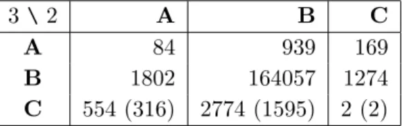
The number of A-branes with negative P and Q tadpoles in configurations of types [p, 0, 0, 0] and [p, q, 0, 0] is tabulated in Table 2. So, for example, of the 57,651 combinations with 3 A-branes, 857 are of type [3, 0, 0, 0], 52,761 are of type [2, 1, 0, 0], and the remaining 4033 are of type [1, 1, 1, 0].
While there are only 226 individual A-branes which alone satisfy all tadpole con-straints, many more distinct individual A-branes are possible in combination with other A-branes. The number of distinct (up to symmetry) A-branes appearing in any configu-ration is 3259. A simple consequence of the Two Column SUSY Bound (3.5) is that no
p\q 0 1 2 3 1 226 28560 - -2 1695 52761 3286 -3 857 5048 694 51 4 105 689 170 0 5 9 89 27 0 6 2 12 0 0 7 1 0 0 0 8 1 0 0 0
Table 2: Number of configurations with p A-branes with negative P tadpole, q A-branes with negative Q tadpole, and no branes with negative R or S tadpole.
individual A-brane can have more than one tadpole > T . It is possible, however, to have an A-brane with one large positive tadpole, compensated by a negative tadpole on another brane. The most extreme case of this is realized in a two A-brane combination in which one brane has a tadpole P = 800
(−792, 3, 3, 88)(3,1;3,1;−88,−1) + (800, 2, 5, −80)(2,1;5,1;80,−1). (3.18) One of the most significant features of the A-brane combinations tabulated in Table 1 is that
Any combination of A-branes has at most one negative total tadpole
This was proven in [21] for a combination of two A-branes but it is straightforward to generalize to any number of A-branes. Consider for example the tadpoles P, Q. As in the discussion in2.3, for every brane with negative Pa= −P we have from the SUSY condition
Qa/j − P/h > 0, and for each brane with negative Qb = −Q we have −Q/j + Pb/h > 0.
Thus, in the sum over all branes in any configuration we have X a Pa h + Qa j > 0 (3.19)
so that only one of the total tadpoles P, Q can be negative. The same holds for any pair so, as stated above, at most one total tadpole can be negative for any combination.
As a consequence of this result, any combination of A-branes acts in a similar fashion to a single A-brane. Furthermore, when A-branes are added, since the individual wind-ing numbers on each brane must be smaller, the maximum achievable negative tadpole decreases quickly as the branes are combined. Thus, a single A-brane can achieve the most negative tadpole. Indeed, the single A-brane with the most negative tadpole (and no tadpoles > T ) is
(−512, 8, 8, 8)(8,1;8,1;−8,1). (3.20)
The combination of two A-branes with the most negative total tadpole is
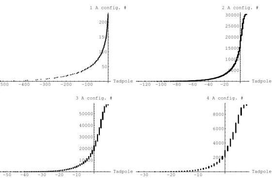
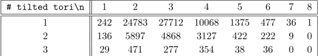
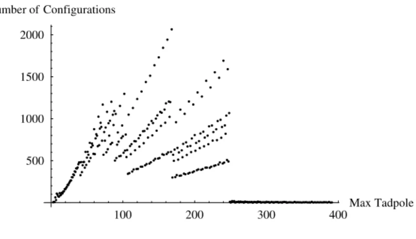
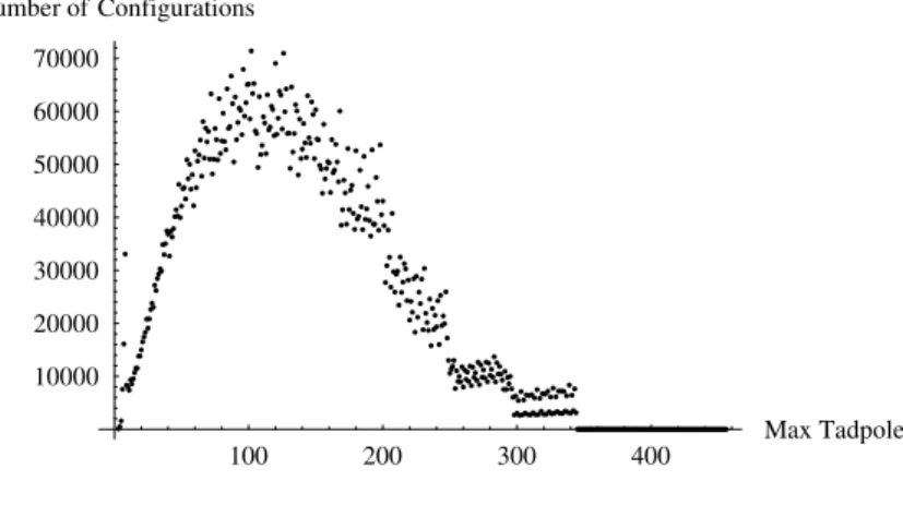
-500 -400 -300 -200 -100 Tadpole 50 100 150 200 1 A config. # -120 -100 -80 -60 -40 -20 Tadpole 5000 10000 15000 20000 25000 30000 2 A config. # -50 -40 -30 -20 -10 Tadpole 10000 20000 30000 40000 50000 3 A config. # -30 -20 -10 Tadpole 2000 4000 6000 8000 4 A config. #
Figure 1: Minimum total tadpole in each configuration of 1, 2, 3, and 4 A-branes (untilted tori).
For three A-branes, the most negative total tadpole is -54, and for four A-branes the most negative total tadpole is -32. The distribution of the smallest total tadpole for all combinations of 1-4 A-branes (with no total tadpoles > T ) is depicted in Figure1. In each case, the branes are ordered by minimum total tadpole and distributed linearly along the vertical axis.
We thus see that most multiple A-brane configurations have similar properties to a single A-brane with a minimum tadpole which is fairly small in absolute value. Only for combinations with a small number of A-branes are there configurations with substantially large negative tadpoles. Note, however, that although multiple A-brane configurations act similar to a single A-brane in terms of the total effect on tadpole contributions, they may act very differently when it comes to satisfying K-theory constraints.
In constructing more general models with multiple stacks of D-branes, the greatest variety of constructions is possible when the smallest total tadpole coming from the A-brane sector is as negative as possible. In particular, the greatest flexibility in adding B-branes and C-branes is afforded when the A-brane sector has a very negative total tadpole and the positive total tadpoles are also small. This is realized primarily for single A-branes with very negative tadpoles. There are 33 single A-branes with negative tadpole ≤ −128, and 71 single A-branes with negative tadpole ≤ −54. A typical example is the A-brane
(−168, 3, 7, 8)(3,1;7,1;−8;−1). (3.22)
There are also 403 combinations of two branes with negative tadpole ≤ −54. The two A-brane combinations have larger positive total tadpoles than the single A-brane configurations with similar negative tadpole, so that the single brane gives space for a wider variety of
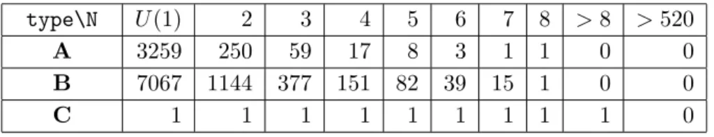
# tilted tori\n 1 2 3 4 5 6 7 8
1 242 24783 27712 10068 1375 477 36 1
2 136 5897 4868 3127 422 222 9 0
3 29 471 277 354 38 36 0 0
Table 3: Number of configurations of n A-branes having all total tadpoles ≤ T = 8 with 1, 2, or 3 tilted tori.
added B- and C-branes. As we shall see, most of the diversity of models with multiple brane stacks comes from these single (and some double) brane configurations with highly negative tadpoles. These configurations are also associated with relatively large integer moduli h, j, k, l, as we discuss in more detail in Section 5. On the other hand, as we discuss in Section4.5, the K-theory constraints become more restrictive for single A-branes with very large negative tadpoles. This effect mitigates to some extent the role of the single A-branes with extremely negative tadpoles in generating diversity in constructions of interesting physics models.
Finally, we discuss the question of A-brane combinations with tilted tori. As described in Section2.2, on a tilted torus the tadpole and winding number conditions are very similar to those on a rectangular torus, but the winding numbers on the tilted torus must satisfy ni ≡ 2 ˜mi (mod 2). The relative primality condition is weakened so that ni and 2 ˜mi can
both be even, if ni/2 6≡ ˜mi (mod 2). We can realize all brane combinations realizing these
constraints by simply constructing all brane combinations for the rectangular torus, relating mi in the construction to 2 ˜mi and imposing the additional condition that on a tilted torus
there must be an even number of any brane with ni 6≡ mi (mod 2), corresponding to half
that number of branes with twice the ni and ˜mi equal to that mi. (For several tilted tori,
each tilted direction in which ni 6≡ 2 ˜mi requires that we double the effective number of
branes in the counting for rectangular tori to get a single brane on the tilted tori). Note that when a subset of tori are tilted, the permutation symmetry on tadpoles is broken. In particular, this means that a brane configuration on rectangular tori may give several configurations with 1 or 2 tilted tori, depending on which torus/tori is/are tilted. For example, the single A-brane of (3.22) is a valid A-brane (using mi → 2 ˜mi on the tilted
tori) if either the first or second torus is tilted, but not if the third torus is tilted since n36≡ 2 ˜m3 (mod 2). If we are counting all A-brane combinations with the first torus tilted,
then, after using the permutation symmetry (3.22) gives the allowable A-branes
(−168, 3, 7, 8)(3, ˜1/2;7,1;−8;−1), (−168, 7, 3, 8)(7, ˜1/2;3,1;−8;−1) (3.23) where the tilde denotes winding numbers ˜mi on the tilted torus. We have computed the
number of A-brane configurations with 1, 2, and 3 tilted tori in this fashion. The results are given in Table3.
4. Models containing gauge group G
it is possible to efficiently generate all brane configurations which realize many features of interest. In particular, given any fixed gauge group G it is possible to construct all distinct brane combinations which realize this gauge group as a subgroup of the full gauge group in any model in polynomial time. In principle, construction of all SUSY models is possible, but this is computationally intensive as the total number of models is quite large.
There are several reasons for focusing on the problem of constructing all realizations of a fixed group G rather than simply enumerating all models. This approach significantly simplifies the computational complexity, while still extracting some of the most interesting data. From a purely model-building perspective, say one is interested in constructing all standard-model like brane configurations. For a given realization of the group G321 = SU (3) × SU (2) × U (1) in terms of a set of 3 + 2 + 1 branes, there may be a large number of ways of completing the configuration to saturate the tadpole equations. But much of the physics of the model, such as the number of generations of “quarks” carrying charge under SU (3) and SU (2) depends only on the choice of branes to realize G and is independent of the way in which this model is completed with extra branes. The extra branes may generate a hidden sector or chiral exotics which are of interest, but it is probably more efficient for model building purposes to first consider all realizations of G, and then to explore the possible extra sectors only of those realizations which have physical properties of interest.
From a more general point of view, the purpose of constructing all configurations with fixed gauge subgroup G is to get a clear handle on what the important factors are which control the distribution of models. By considering the variety of ways in which a gauge subgroup like G = SU (3) × SU (2) can be realized in any SUSY IBM model on T6/Z2× Z2, for example, we gain insight into the mechanism responsible for generating the bulk of these configurations. This also provides a clear way to analyze more detailed features of these constructions such as the number of generations of matter fields in various representations. In the first part of this section (Subsection 4.1) we describe the general method of computing all brane configurations which generate a gauge subgroup G; we then explicitly compute all such configurations for gauge groups U (N ) in Subsection4.2and SU (3)×SU (2) in Subsection 4.3. By looking at the distribution of these gauge groups and associated tadpoles, we gain insight into how the diversity of realizations of these groups is associated with A-branes with large negative tadpoles, as well as providing useful tools for model building. We also construct all brane configurations realizing SU (N ) × SU (2) × SU (2) in 4.4. In4.5we discuss the K-theory constraints and how they can reduce the total number of allowed realizations of any fixed G. Finally, in subsections 4.6 and 4.7 we relate the results described here to earlier work on IBM model building on this and other toroidal orbifold models.
4.1 Systematic construction of brane realizations of G
As mentioned above, the problem of finding all ways in which a fixed group G can be realized as a subgroup of the full gauge group can be solved in a straightforward way in polynomial time given the results of the Section 3. Any complete model containing a set of branes individually satisfying the SUSY constraints for a common set of moduli and
collectively solving the tadpole and K-theory constraints, contains either no A-branes or some given set of A-branes which must be one of the 99,479 configurations enumerated above. Given a configuration of A-branes, there is a finite number of ways in which B-and C-branes can be added to saturate the tadpole conditions, since the B- B-and C-branes have only positive tadpoles. Thus, to determine all realizations of G, we just need to run through each of the roughly 105 possible A-brane combinations and for each determine all realizations of G through adding B- and C-branes to the given A-brane combination without oversaturating the tadpole constraints.
To be explicit, say we want to find all models containing the gauge group G = SU (N1)× SU (N2)×...×SU (Nr). Each of the r stacks can be made up of A , B or C type branes (for A- and B-branes SU (Ni) would be realized as a subgroup of U (Ni), while for C-branes, SU (Ni) would be realized as a subgroup of a symplectic group Sp(N ) as discussed in more detail below).
The first step in explicitly constructing all realizations of G is looping through our list of all A-brane configurations. For each A-brane configuration we see if there are Ni duplicates of any brane. If so, then these Ni A-branes can provide a factor of U (Ni) to the gauge group. We form all possible combinations of branes in the A-brane configuration which can be used to compose parts of the group G, with the remaining parts arising from extra branes which must be added to the model. For each of these realizations of a subgroup of G by some branes in a configuration of A-branes, we then consider all possibilites of B and C type branes that can be added in stacks to fill out the remaining needed components of G.
Algorithmically, adding B-branes to the configuration of A-branes is straightforward. Since we have already included all the A-branes that will go into the configuration, and since B-branes have only positive tadpoles, all the tadpoles will be bounded by the tadpole constraint. Thus, to find all ways of including a stack of B-branes which are compatible with a given A-brane combination, we proceed by scanning over possible winding numbers of the B-brane to be added that are consistent with the tadpole constraints. Once a compatible stack of N B-branes is found, we check to see if this B-brane along with the branes already in the configuration satisfy the SUSY condition, by confirming that the resulting constraints on moduli are compatible. All possible ways of adding B-brane stacks within the tadpole constraints can be constructed in this fashion. The addition of stacks of C-branes is even simpler, since there are only four different C-branes that can be added and the C-branes do not affect the SUSY conditions.
After constructing the set of all realizations in this way, we may have multiple instances of the same realization, for example associated with different extra A-brane configurations. To reduce the final set of configurations to a single instance of each equivalent realization, we must drop the extra branes, put each configuration in some canonical form, and drop copies. Note that in this class of brane configurations we have a clear criterion for determining equivalence of solutions, using the symmetries described in Section2.2, unlike for example the situation described in [23].
Thus, in a straightforward way we can scan over all possible inequivalent ways of building the gauge group G from A-, B-, and C-brane stacks in a way which is compatible
with the supersymmetry and tadpole constraints. Note that we are not checking the K-theory constraints at this stage, since we are only generating a subset of the complete set of branes in any given model. Thus, the set of realizations generated through this algorithm may be over-complete. While generically additional branes can be added in many ways, some of which will satisfy the K-theory constraints, in some cases, particularly when our realization of G comes close to satisfying the tadpole constraints, there may be no complete model containing this realization which satisfies the K-theory constraints. This must be checked in a case-by-case fashion for models of interest.
We have so far concentrated on the case when the tori are untilted. For tilted tori we proceed as discussed above for enumerating A-brane stacks. We only keep configurations where there are an even number of branes with ni 6≡ mi = 2 ˜mi on the tilted tori, noting that the resulting gauge group for a stack of 2kN such branes with ni 6≡ mi on k tilted tori is U (N ). Practically, we can find configurations realizing a desired gauge group on a compactification with tilted tori by computing the configurations on untilted tori, and then checking whenever there is a stack of N branes with ni 6≡ mi on k tilted tori that an additional N (2k − 1) branes of this kind can be added without oversaturating the tadpole conditions. (For the A-branes, we just need to confirm that there are an additional N (2k− 1) of these branes available in the A-brane combination used at the first step of the analysis.) Clearly, this means that with more tilted tori there will be fewer realizations of G.
4.2 Realizations of SU (N )
As a simple example, we consider the construction of all possible brane realizations of the group SU (N ) as a subgroup of the full gauge group. There are 3 ways in which the group SU (N ) can be realized.
i) The group SU (N ) can be realized as a subgroup of the U (N ) associated with N identical A-branes5. To identify all ways in which this can be done we just need to scan over all 105 known A-brane combinations for configurations including N copies of the same brane, and then list all A-branes for which N copies appear in some A-brane combination. ii) The group SU (N ) can be realized, again as a subgroup of U (N ), through N identical B-branes. For each combination α of A-branes, we look at all possible ways in which a B-brane β can be chosen so that combining N copies of β with α gives total tadpoles which are all ≤ T . This condition puts strong constraints on the winding numbers of β. For each β which combines with α without exceeding the tadpole constraints, a further check must be done that the system of linear equations given by the SUSY equalities (2.6) for the branes in α and β admit at least one solution. Finally, symmetries must be considered so that only one example of each such β configuration is included in a final list. (While the same brane stack β may be associated with many different A-brane combinations α, these represent “extra” branes in the same way as additional B-branes or C-branes completing 5Note that when SU (N ) is realized as a subgroup of U (N ), as in i) and ii), the extra U (1) factor often
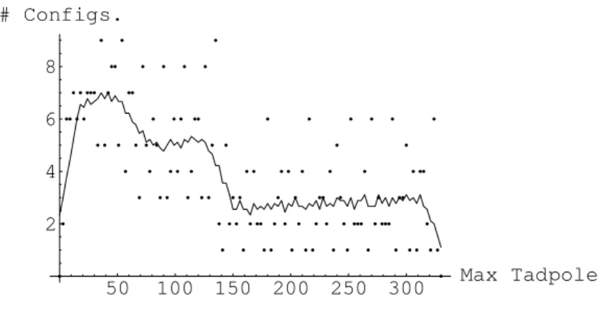
type\N U (1) 2 3 4 5 6 7 8 > 8 > 520
A 3259 250 59 17 8 3 1 1 0 0
B 7067 1144 377 151 82 39 15 1 0 0
C 1 1 1 1 1 1 1 1 1 0
Table 4: Numbers of distinct ways in which SU (N ) (U (1) for N = 1) can be realized by A, B, or C-type branes as a subgroup of the full gauge group (with untilted tori).
the tadpole constraints, so do not really realize distinct realizations of SU (N ).)
iii) The group SU (N ) can also be realized as a subgroup of Sp(N ) arising from N identical C-branes. Checking for this possibility for each combination α of A-branes is straightfor-ward; any total tadpole of α which is less than T − N can be associated with N additional C-branes. The value N = 2 is a special case, since SU (2) = Sp(1), so SU (2) can be real-ized from a single C-brane. Since there is really, up to symmetry, only one possible stack of N C-branes, there is one possible realization of each SU (N ) as a subgroup of Sp(N ) up to the maximum of N = 520, which can be realized in the presence of the A-brane (3.20). There is one more subtlety here relevant for model-building. Although the group SU (N ) can be realized as a subgroup of Sp(N ) with N C-branes, the fields transforming only under that Sp(N ) live in the antisymmetric representation and cannot break Sp(N ) down to only SU (N ). By turning on bifundamentals, for example between two stacks of N C-branes with different tadpoles, the symmetry can be broken down to SU (N ); this cor-responds to brane recombination, giving a different set of branes. Alternatively, if we have 2N C-branes, these branes can be moved away from the orientifold plane, giving a gauge group U (N ) ⊃ SU (N ), as described in [16]. Using this mechanism, the largest SU (N ) which can be realized without the remainder of an Sp(N ) is SU (260) by 520 C-branes in combination with (3.20).
We have carried out the necessary computation for each type of brane. The number of distinct realizations of SU (N ) in terms of A-branes, B-branes, and C-branes is shown in Table4.
Most of the realizations of SU (N ) arise from stacks of N B-branes. To understand the origin of the numbers in this table more clearly let us consider the case of SU (7) ⊂ U (7) arising from 7 identical B-branes. Each B-brane has two nonvanishing tadpoles, so up to symmetries the B-brane involved has tadpoles (P, Q, 0, 0) with P ≥ Q > 0, so the full U (N ) stack has total tadpole (7P, 7Q, 0, 0). Since every A-brane combination has at most one negative tadpole, we must have Q = 1. This constrains the winding numbers n1, m2, m3 to
be unity (with canonically chosen signs), so that the only freedom is in winding numbers n2, n3 with P = n2n3. In the absence of any A-branes, we can only have P = 1. Any
A-brane combination included must have total Q = 1, and P < 0. Among single A-branes, the one with the most negative tadpole and Q = 1 is
α64= (−64, 1, 8, 8)(1,1;8,1;−8,−1). (4.1)