Integrity of an autonomous agricultural vehicle according the definition of trajectory traversability

HAL Id: hal-00557038

https://hal.archives-ouvertes.fr/hal-00557038

Submitted on 18 Jan 2011

HAL is a multi-disciplinary open access archive for the deposit and dissemination of sci-entific research documents, whether they are pub-lished or not. The documents may come from teaching and research institutions in France or abroad, or from public or private research centers.

L’archive ouverte pluridisciplinaire HAL, est destinée au dépôt et à la diffusion de documents scientifiques de niveau recherche, publiés ou non, émanant des établissements d’enseignement et de recherche français ou étrangers, des laboratoires publics ou privés.

according the definition of trajectory traversability

C. Debain, P. Delmas, R. Lenain, Roland Chapuis

To cite this version:

C. Debain, P. Delmas, R. Lenain, Roland Chapuis. Integrity of an autonomous agricultural vehi-cle according the definition of trajectory traversability. AgEng 2010, International Conference on Agricultural Engineering, Sep 2010, Clermont-Ferrand, France. p. - p. �hal-00557038�

Integrity of an autonomous agricultural vehicle according the

definition of trajectory traversability

Christophe Debain*, Pierre Delmas*, Roland Lenain*, Roland Chapuis**

e-mail: christophe.debain@cemagref.fr

(**) LASMEA - UMR 6602, 24, avenue des Landais, 63177 Aubiere, France

Abstract

In this article we address the problem of the traversability of the trajectory of an agricultural robot defining the conditions insuring a safe displacement according the notion of "obstacle". Unlike other approaches that try to detect and to avoid obstacle, we propose the concept of Allowable Speed Trajectories which depends on the vehicle capabilities, its dynamics constraints, its speed and the 3D rendering of the environment. We make a dynamic study to estimate the acceleration of inertial center of vehicle taking into account geometry of the environment and the trajectory to follow. Then we propose some solutions to adapt the speed and/or the trajectory of the agricultural vehicle according criteria linked to the mission objective. Results in simulation and real conditions show the performance of our algorithm in different scenarios.

Keywords:

autonomous vehicles, traversability, obstacle avoidance

1. Introduction

The management of mobile robots in highly unstructured outdoor environments as agricultural applications (figure 1) is still an open issue. Many teams in the world are working on this subject addressing different research domains. Kelly in [1] introduces the difficulties encountered when autonomy is given to a vehicle that must move in real contexts. Lots of scientific problems have to be considered in this wide subject as perception of the environment [2], control in difficult situation like sliding terrains [3] with stability insurance

[4], obstacle avoidance [5].... All these subjects are essential and have to be considered in an elegant manner in order for the system to be efficient and reliable. Since 2004, our team has decided to address these problems from a new point of view: Since the beginning of the robotic domain, the most part of the research teams have considered the robotic problems from the sensors point of view. For instance,

when they want to localise a robot, they use a sensor like a GPS receiver (global localisation) or a camera (local localisation). Then, powerful algorithms are developed to extract features and the result is the input of the control algorithm in order to automatically drive vehicles. This often requires a substantial computing resources, and these algorithms are difficult to use outside their experimental contexts.

Our team works in the opposite way: We consider the autonomy of the robot and we try

Figure 1: cereal harvest

to determine what is useful for this autonomy. For automatic guidance it means: what should be the precision of the guidance process (perception and action)? What should be confidence on this precision? What physical integrity of the robot (traversability of its trajectory and confidence on this traversability)? What safety... The most important improvement of our solution is to put these elements in the center of our methodology. The main idea in this concept is to call a resource (sensor or algorithm) when it is necessary evaluating the ratio between gain and cost of each resource. If all the needs of the robot are fulfilled no resource are called. This concept has been used for the first time [6] to automatically guide a small vehicle (see figure 2). If no "obstacle concept" is considered in this first application, the automatic adaptation to different context and the reliability of the demonstration were particularly appreciated.

In this article we present the results of our concept through an application which consists of the preservation of the physical integrity of a vehicle when it moves automatically. Like for the automatic guidance process, we don't look for an obstacle on the trajectory of the robot but we want to define the conditions insuring a safe displacement of the robot. So after a first part giving the main methods usually applied for safe navigation, we detail our method based on the system requirements for safe automatic guidance systems. In the third part we show some results in simulation and real conditions before concluding with our future works.

2. Previous Works

Safe navigation of mobile robots in outdoor environment is addressed by numerous studies that we classify into two categories: Reactive obstacle avoidance methods and Dynamic characteristics to evaluate admissible speed.

Reactive obstacle avoidance methods

The initial works on safe autonomous navigation were those dealing with reactive obstacle avoidance. Indeed, the idea is to preserve the physical integrity of the mobile robot by avoiding dangerous elements commonly called "obstacles".

The most famous use of this idea is the method of Potential Fields [5.] It consists of building potential functions which resume the navigation objectives. An obstacle is represented by a repulsive field and the goal to reach by an attractive field. Therefore, for every position of a mobile robot, a resulting force exists from potential fields which indicates the direction to follow. Although this method is purely reactive, it needs few computing resources but it can create a local minimum problem with U-shape obstacle. Moreover, this method can lead to oscillation problems when the vehicle is in a narrow corridor.

An other method is the Vector Field Histogram (VFH) [7] and its improvements (VHF+,VHF*) which result from Potential Field method. It consists to represent the evolution space of mobile robot in a weighted grid. Every cell is affected by the probability of obstacle occupation. Then, it is possible to determine a free path and the control to apply.

The Dynamic Windows Approach [8] allows to select the best match (speed and rotation) which allows the mobile robot to avoid obstacle including kinematic and dynamic constraints. This match produces a circular trajectory which allows to evaluate the different constraints. The main inconvenience of this method is the choice of the speed space sampling. For real-time applications which address different speeds of robot, it may be difficult to define a resolution of the speed space compatible with real-time constraints and stability criteria. An other method is the Nearness Diagram [9]. It consists of building two diagrams of obstacle proximity. The Point Nearness Diagram represents the distribution of obstacle around the vehicle. The Robot Nearness Diagram represents the same distribution but in relation to the security area of mobile robot. Thanks to these diagrams, the vehicle can

analyse its situation among previously defined ones and uses the associated solution. As this method analyses in which case it is, it needs a lot of computing times.

All of these methods try to avoid obstacles with real-time constraint but they require the observation of a significant part of the robot environment considering most of the detected elements as an obstacle. Consequently, the solutions are only stopping the vehicle or avoiding the disruptive elements.

However, the obstacles definition takes no account of capabilities and dynamics of the vehicle. Yet if we consider the dynamics of the mobile robot, "obstacles" are not always damaging. By example, a road bump is not dangerous for a car at low speed but it becomes at high ones.

Dynamic characteristics to evaluate admissible speed

The progress made in recent years regarding control laws for high speed navigation of mobile robot (an example in [10]) reach a level where dynamic characteristics of the robot become important. They can be used to improve the control accuracy but also to estimate the admissible speed to ensure the safety of robots. The study proposed in [11] models a UGV (Unmanned Ground Vehicles) in a elementary manner to determine the effect of obstacle height on major design parameters, such as the wheel size, the wheelbase and the gravity center. But, this analysis gives results only for crossing a step in outdoor environment. However, in agricultural field many kinds of obstacle have to be considered. We have to address other characteristics like slope and more generally the shape of the ground.

In [4] Bouton proposes a safe navigation system for users of all-terrain vehicles. Thanks to kinematic and dynamic characteristics of the vehicle the system predicts rollover and indicates the hazardous situations to the drivers. Although this study is limited to the rollover, it shows a great potential to increase safety of autonomous robots. A last example is given in [13] where authors use the physical model of a mobile robot to determine the admissible speed and acceleration insuring the integrity of the robot. However because of the complexity of the modelisation, the result of this work is not applicable in a real time application like an automatic guidance system for agricultural vehicles.

Conclusions

This first part addresses various ways to improve the physical integrity of mobile vehicle moving in outdoor environments. The main drawback of these methods is not to define what constitutes an obstacle that means what part of environment may disturb the integrity of the robot taking into account its dynamic parameters. Some methods try to include dynamic parameters of vehicles to estimate the conditions of their integrity but they are for specific case or they are too theoretical to be used in real application for agricultural vehicles.

In this paper, we propose a method to provide safe navigation to agricultural vehicles taking into account dynamic parameters and capabilities of the vehicles in the context of a real application of automatic guidance.

3. Description of the Automatic Guidance System

As introduced previously, our automatic guidance system does not search to avoid a possible obstacle but tries to evaluate the admissible speed to cross the environment. To do that, we first have to consider the trajectory of the robot in its environment. It means selecting the part of the environment of the

robot that includes its trajectory. Then, we have to analyse the variation of physical state of the robot to estimate the admissible speed profile of its trajectory. To finish, the system must choose the best navigation strategy (direction and vehicle's speed).

The algorithm described in details in this paper can be summarized as follow:

Admissible Path Generation

In this part we consider that the robot has to follow a trajectory (reference trajectory) included in a small corridor in which the robot can move. So the robot can decide to move away from the reference trajectory but only if its new route is included in the corridor. For this, the system has to predict various eligible paths within the constraints of vehicle dynamics and included in the navigation corridor. Although the navigation corridor limits the number of admissible paths, this last one is too big to analyse all of the possibilities. So, we decide to generate only path which are the most useful in regard to the application. That is why, we chose to evaluate

only few paths which are parallel of the reference one. To resume, at each iteration of the system, the first step is to evaluate the evolution of the position to reach the different paths selected in the corridor (figure 3).

The corridor is defined by the user at the same time as the reference trajectory. To build the admissible paths we chose to use the popular Ackerman’s model [12]. The state vector of the system at the moment k is Sk = (Xk, Yk, θk, δk)T with (X, Y) the position of the vehicle in global coordinate frame, θ its orientation, and δ its front wheels direction. The evolution equation of the mobile robot S(k+1) =

f(Sk,Uk) is defined in the equation (1) where Uk = δck is the wheel direction set point, L is the axle spread of the mobile robot and ∆S is the iteration distance for the prediction.

The system manages a real vehicle that is why we decide to make an approximation of wheels direction equation by a first order system.

Consequently the constant where ∆T represents the iteration time of the system, and τ_wd is the time constant of the first order system.

To generate one path (Pi) the system calculated the best until the end of a horizon time. We chose to use discrete quadratic optimal control law with over horizon time Nc to compute this path generation. Because of the nonholonomic constraints of our agricultural vehicles, we propose to minimise the lateral and angular deviation between the mobile robot and the selected path.

The principle is to calculate the Nc controls minimizing a criteria. The criteria to minimize (JPi ) may be defined by the equation (2):

Figure 3 : The vehicle has few optional objectives. They are the reference and parallel paths

where Q are weighted matrix, R the cost of the control, Sn,Pi the position and the orientation of the followed path and Nc the time horizon to calculate the sequence:

To compute Sn,Pi , we search the nearest point between the nominal path and the mobile robot position. θ_n,Pi corresponds at the tangent at this point. Then, the system estimates by the straight lines which are tangent at the reference path at the point .

Now, the system is able to determine the sequence

in order to generate the points of the generated trajectories in the corridor. It repeats the same algorithm until the end of the prediction time.

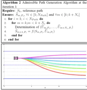
We may resume this level by the algorithm 2: At the end of this level, the system has generated different admissible paths in the corridor. Due to the used model, these paths match with kinematic constraints of the mobile robot.

An example is given by the figure 4:

To check the practicability of these paths, the system must calculate the pitch, roll and yaw for each generated points using a Digital Elevation Map (DEM) of the environment.

Prediction Physical Vehicle State

The system has previously generated several possible trajectories for the vehicle travelling in a corridor. Now, it has to predict the physical state of the mobile robot for the points of each trajectory (pitch, roll, yaw). To do that, the system uses an elevation grid of the nearby environment. It then determines the position of each wheel for each generated point. Wheels position is calculated by the equation (3).

(3)

with Pwk,Pi is the position of the four wheels at point , Pwl constant matrix which represents wheels positions on the vehicle’s frame, and MRot the rotation matrix between the frames at the beginning of prediction and the frame at moment k (figure 5).

Then, the physical state of the mobile robot is obtained by projecting positions of each wheel at each instant in the elevation map.

The system may after calculate the first and second derivatives by curvilinear abscissa of physical state.

However there are many cases where the vehicle is unable to follow the path selected. The first one is given by one of our hypothesis: the mobile robot can't cross over a step bigger than 1/3 of diameter

Figure 4: Result after path generation level

Figure 5: Projection of generated path on the DEM

of its wheels. Consequently, if the system observes a variation bigger than 1/3 of diameter of wheel for one wheel of the vehicle, the system stops and it calculates another path.

Another condition is that all wheels must touch the ground. To check this condition, we calculate the error between elevation of wheels

obtained by the projection on the DEM and the projection of the median plane (figure 6). If this distance is bigger than suspension clearance (SC), we consider that it is impossible that all wheels touch the ground.

The last condition to respect is about the size of chassis of the robot. The system must check that the chassis of the vehicle does not touch the ground. So, we calculated the distance between DEM and median plane calculated previously. If this distance is upper than height of chassis, the path is not practicable for the vehicle.

Prediction Admissible Speed Profile

The system has calculated the admissible path, and then it determined the physical state of the vehicle by the projection of wheel position on the DEM. Moreover, it has checked if all the selected paths are practicable in relation to the size of the mobile robot and wheel diameter. Now, we have the principle elements useful to determine the admissible speed profile for each selected path.

To do that we propose to use the method defined in a previous work [14]. The principle is to calculate the acceleration of the inertial center of the vehicle (AG/R0) in relation to the variation

of the physical state and the linear speed of the vehicle. Then, the system determines the maximum linear speed which permits that the projection of the inertial center stays in the polygon defined by the support (figure 7).

At the end we obtain the admissible speed profile for each selected path.

Path and Control Selection

To resume, the system has generated few paths, it has calculated the physical vehicle state for each one and determinate their admissible speed profile. Now, the system must choose the best path it will follow.

To choose the best path of the vehicle, the system uses the criterion J whose goal is to select the path closer to that of the reference trajectory and with a speed profile close to the reference speed.

Figure 7: Condition to calculate the admissible speed. The vector R= AG/R0+P must stay in the blue area

Figure 6: Checking of contact between vehicle’s wheels and the elevation grid

Consequently, the criterion represents the area between reference path and path Pi (APi) and

the area between reference speed and admissible speed profile (A_ASP,Pi). However, with

this criterion we observe the choice is not stable. To avoid this problem we decide to add the same criterion used for the generation path (JPi). This term can be considered like the cost to

reach each different path. The criterion Jselection is explained in the equation (4).

(4)

At the end, when the path is selected, the vehicle uses the control set point of this path. At the next iteration of the system, it will start again its cycle with its new position. If no path is admissible, the system stops the vehicle.

4. Results

Previously, we have a first result shown in [14] (to see the video [17]) where the vehicle manages its speed to cross over a bump (figure 8).

This bump is crossable at vehicle speed less than about 0.5m/s. We can notice a good behaviour of the mobile robot during this experimentation because it stays on the nominal path and decreases its speed to respect the speed profile. After crossing the bump, the vehicle increases its speed until the reference one (5m/s).

However, for this test we give to the system the position and the characteristics of the bump because we have not yet a perception system adapted to our control algorithm.

To show more results in this article we propose to use a robotic simulator which is able to simulate 3D environment, physics of simple vehicles, and few sensors like camera, kinematics GPS... Contrary to behavioural simulator, this one manages a realistic 3D graphic engine, a physical engine modelizing the reaction of mobile robot and a real-time middleware. It was developed with 2 open source C++ library: OGRE 3D (see [15]) which is a 3D graphic rendering engine for the visual part and ODE (Open Dynamic Engine, see [16]) a physical engine which manages the collision with the environment and the physical model of the vehicle. The real-time middleware which wraps the all is AROCCAM. AROCCAM manages the data sensor flux, and the vehicle's actuators between the simulator and the control algorithms. The main advantage of this robotic simulator is that we can first test our algorithm in a realistic environment. Thanks to the robotics properties of our simulator, the control software executed by the simulator is exactly the same than the one embedded on the real vehicle.

In simulation conditions, numerous validation procedures are possible. If we made lots of tests with canonical scenarios we chose here one as realistic as possible (see figure 9). The ground is not flat and the shape of environment is unstructured. For this test, the reference vehicle speed is 5m/s and the navigation corridor width is 8m. The reference path crosses a depression on the floor which is impossible to practice for the vehicle. We can notice that the system succeeds in managing automatically its speed and its wheels direction maintaining the physical integrity of the vehicle (see video at [18]).

Figure 8: First test of our control system with our electrical vehicle AROCO

Figure 9: Snapshot of simulated test with a realistic map,

in red: forbidden trajectories, in orange: reference trajectory, in green: admissible trajectories

5. Conclusion and future works

Conclusion

In this paper, we proposed to let out the method of obstacle avoidance. Unlike classical methods of obstacle avoidance, we try to analyse the geometric shape of the environment and to determine the admissible speed allowing the vehicle to eventually cross the considerate area. At each iteration, the system computes different possible paths in a corridor, and it evaluates their practicability taking into account vehicle capabilities. Then, it chooses to follow the best one in relation to a criterion which depends of the application. In this paper we show different tests in simulation and in real conditions. Most of them have been done in simulation in order to test numerous scenarios and canonical situations. All of them have proven the efficiency of our system to preserve the physical integrity of the vehicle and to select the best trajectory in regard to a criterion defined by the application.

Future works

The next step of our work is to adapt this automatic guidance system to the work about environment perception done by Malartre in [19]. In this work a fusion process between camera sensor and a rangefinder is proposed (see figure 10). However, in this paper, we have made the hypothesis that the perception part is perfect. But in real case, the maximum distance of perception and the precision of the measurement are limited. So, the guidance part will have to adapt the navigation strategy in relation to this lack of perception performance. We will then talk about "caring control". Finally, our automatic guidance system will converge to the best navigation strategy thanks to the minimization of a perception-guidance function.

REFERENCES

[1] A. Kelly and A. Stentz, ”Minimum Throughput Adaptive Perception for High Speed Mobility”, in IEEE/RSJ Int. conf. on intelligent robots and systems 1997, Grenoble, France, 1997.

[2] F. Chanier, P. Checchin, C. Blanc, and L. Trassoudaine, ”Map fusion based on a multi-map SLAM framework”,In Proceedings, IEEE International Conference on Multisensor

Fusion for Intelligent Systems, Seoul, Korea, August 2008.

[3] C. Cariou,R. Lenain,B. Thuilot and P. Martinet, ”Adaptive control of four wheel steering off road mobile robots: application to path tracking and heading control in presence of sliding”, in

IEEE/RSJ Int. conf. on intelligent robots and systems (IROS), Nice, France, September

22-26, 2008.

[4] N. Bouton,R. Lenain,B. Thuilot and P. Martinet, ”A rollover indicator based on a tire stiffness backstepping observer: application to an all-terrain vehicle”, in IEEE/RSJ Int. conf.

on intelligent robots and systems (IROS), Nice, France, September 22-26, 2008.

[5] O. Khatib, ”Real-time obstacle avoidance for manipulators and mobile robots”,

International Journal of Robotic Research, vol. 5, No. 1, 1986, pp 90-98.

[6] C. Tessier, C. Debain, R. Chapuis and F. Chausse, ”A cognitive perception system for autonomous vehicles”, International Conference of COGnitive systems with Interactive

Sensors 2007, Stanford University, California, USA, 2007, 7p.

[7] J. Borenstein and Y. Koren, ”The Vector Field Histogram – Fast Obstacle Avoidance for Mobile Robots”, IEEE Journal of Robotics and Automation, vol. 7, No. 3, June 1991, pp 278-288.

[8] D. Fox, W. Burgard and S. Thrun, ”The dynamic window approach to collision avoidance”,

IEEE Robotics and Automation Magazine, vol. 4, issue. 1, March 1997, pp 23-33.

[9] J. Minguez and L. Montano, ”Nearness Diagram Navigation (ND): A New Real Time Collision Avoidance Approach”, in International Conference on Intelligent Robots and

Systems,Takamatsu, Japan, 2000, pp 2094-2100.

[10] R. Lenain, B. Thuilot, C. Cariou, P. Martinet , ”Mixed kinematic and dynamic sideslip angle observer for accurate control of fast off-road mobile robots”, Journal of Field Robotics, vol.27, Issue 2, 2009, pp 181-196.

[11] M. D. Berkemeier, E. Poulson and T. Groethe, ”Elementary Mechanical Analysis of Obstacle Crossing for Wheeled Vehicles”, Proceeding in the IEEE International Conference

on Robotics and Automation, Pasadena, CA,USA, May 2008, pp 2319-2324.

[12] J. Ackermann and W. Sienel, ”Robust yaw damping of cars with front and rear wheel steering,” IEEE Trans. Control Syst. Technol., vol. 1, no. 1, pp. 15-20, Mar. 1993.

[13] M. Mann and Z. Shiller, ”Dynamic Stability of Off-Road Vehicles: Quasi-3D Analysis”,

Proceeding in the IEEE International Conference on Robotics and Automation, Pasadena,

CA,USA, May 2008, pp 2301- 2306.

[14] P.Delmas, N. Bouton, C. Debain and R. Chapuis, ”Environment characterization and path optimization to ensure the integrity of a mobile robot”,Proceeding in IEEE International

Conference on Robotics and Biomimetics, Guilin, China,December 2009.

[15] http://www.ogre3d.org/ [16] http://www.ode.org/

[17] http://most.clermont.cemagref.fr/projets/download/Delmas.wmv/view

[19] F. Malartre, T. Feraud, C. Debain and R. Chapuis, ”Digital Elevation Map Estimation by Vision-Lidar fusion”,Proceeding in IEEE International Conference on Robotics and