HAL Id: hal-00295956
https://hal.archives-ouvertes.fr/hal-00295956
Submitted on 29 Jun 2006
HAL is a multi-disciplinary open access
archive for the deposit and dissemination of
sci-entific research documents, whether they are
pub-lished or not. The documents may come from
teaching and research institutions in France or
abroad, or from public or private research centers.
L’archive ouverte pluridisciplinaire HAL, est
destinée au dépôt et à la diffusion de documents
scientifiques de niveau recherche, publiés ou non,
émanant des établissements d’enseignement et de
recherche français ou étrangers, des laboratoires
publics ou privés.
reactive halogen species in aqueous solution: Part 1 ?
bromide solutions
B. M. Matthew, C. Anastasio
To cite this version:
B. M. Matthew, C. Anastasio. A chemical probe technique for the determination of reactive
halo-gen species in aqueous solution: Part 1 ? bromide solutions. Atmospheric Chemistry and Physics,
European Geosciences Union, 2006, 6 (9), pp.2423-2437. �hal-00295956�
www.atmos-chem-phys.net/6/2423/2006/ © Author(s) 2006. This work is licensed under a Creative Commons License.
Chemistry
and Physics
A chemical probe technique for the determination of reactive
halogen species in aqueous solution: Part 1 – bromide solutions
B. M. Matthew1,*and C. Anastasio11Atmospheric Science Program, Department of Land, Air & Water Resources, University of California, Davis, USA *now at: Hach Company, Loveland, Colorado, USA
Received: 16 November 2005 – Published in Atmos. Chem. Phys. Discuss.: 2 February 2006 Revised: 27 April 2006 – Accepted: 8 May 2006 – Published: 29 June 2006
Abstract. Reactive halogen species (X*=X•,•X−2, X2 and
HOX, where X=Br, Cl, or I) in seawater, sea-salt particles, and snowpacks play important roles in the chemistry of the marine boundary layer. Despite this, relatively little is known about the steady-state concentrations or kinetics of reactive halogens in these environmental samples. In part this is be-cause there are few instruments or techniques that can be used to characterize aqueous reactive halogens. To better understand this chemistry, we have developed a chemical probe technique that can detect and quantify aqueous re-active bromine and chlorine species (Br*(aq) and Cl*(aq)). This technique is based on the reactions of short-lived X*(aq) species with allyl alcohol (CH2=CHCH2OH) to form stable
3-halo-1,2-propanediols that are analyzed by gas chromatog-raphy. Using this technique in conjunction with competition kinetics allows determination of the steady state concentra-tions of the aqueous reactive halogens and, in some cases, the rates of formation and lifetimes of X* in aqueous solu-tions. We report here the results of the method development for aqueous solutions containing only bromide (Br−).
1 Introduction
Gaseous and aqueous reactive halogen species (X*, where X=Br, Cl, or I) play important roles in the chemistry of ma-rine regions. In solution, such as deliquesced sea-salt parti-cles and surface seawater, aqueous reactive halogen species (X*(aq)=X•,•X−2, X2and HOX) are important for a number
of reasons. For example, model studies of the remote ma-rine boundary layer (MBL) have predicted that hypohalous acids (HOBr and HOCl) are significant oxidants for S(IV) in sea-salt particles and MBL clouds (Vogt et al., 1996; Keene and Savoie, 1999; von Glasow et al., 2002b). It has also
Correspondence to: C. Anastasio
(canastasio@ucdavis.edu)
been suggested that the photo-oxidation of halides can lead to the abiotic formation of halogenated organic compounds in seawater (Gratzel and Halmann, 1990; Moore and Zafiriou, 1994) and in polar snowpacks (Swanson et al., 2002).
In addition, halide reactions in sea-salt particles are closely linked to gas-phase chemistry through heterogeneous pro-cesses. For example, sea-salt particles and surface snowpack are important sources of gaseous reactive halogen species such as Br2and BrCl to the MBL (McConnell et al., 1992;
Sander and Crutzen, 1996; Vogt et al., 1996; Michalowski et al., 2000; Foster et al., 2001; von Glasow et al., 2002a). A growing body of evidence indicates that these reactive gaseous halogens significantly influence the global budgets of tropospheric species such as ozone, hydrocarbons and mercury. For example, in Arctic regions springtime ozone depletion and hydrocarbon loss have been linked to Br•and Cl•, respectively (Barrie et al., 1988; Jobson et al., 1994; Bottenheim et al., 2002). The recently described early-morning destruction of ozone in both the mid-latitude and sub-tropical marine boundary layers has also been attributed to halogen chemistry (Nagao et al., 1999; Galbally et al., 2000; von Glasow et al., 2002a). Satellite and ground-based measurements of BrO• (produced from the reaction of Br• with O3)have revealed that the bromine-catalyzed
destruc-tion of ozone is widespread in the troposphere, occurring in the Arctic and Antarctic (Richter et al., 1998), as well as near saline lakes such as the Dead Sea (Hebestreit et al., 1999) and Great Salt Lake (Stutz et al., 2002). In addition to these ef-fects, a recent model of halogen chemistry in the mid-latitude MBL (30◦N) has indicated that dimethyl sulfide (DMS) ox-idation increases by ∼60% when reactions with BrO• are considered (von Glasow et al., 2002b). The deposition of mercury in Arctic and Antarctic ecosystems has also been linked to reactions of phase elemental mercury with gas-phase X•and XO•(Ebinghaus et al., 2002; Lindberg et al., 2002).
Because reactions in the aqueous phase appear to play a large role in the overall chemistry of gaseous reactive halo-gen species, it is important to understand the reactions that form X*(aq). While many past studies of individual halogen radical reactions in aqueous solution have used flash photol-ysis and pulse radiolphotol-ysis, these techniques require equipment that is rather specialized and expensive. An alternative ap-proach is use of a chemical probe in conjunction with com-petition kinetics, a technique that has been used in the past to measure hydroxyl radical (•OH) in seawater, cloud water, fog water, and on ice (Zhou and Mopper, 1990; Zepp et al., 1992; Faust and Allen, 1993; Arakaki and Faust, 1998; Anastasio and McGregor, 2001; Chu and Anastasio, 2005). The goal of this work was to create an analogous technique to mea-sure aqueous reactive halogen species using allyl alcohol (2-propene-1-ol), which reacts with X*(aq) to form brominated or chlorinated diols. As part of this we have developed a ki-netic model, based on known halide radical chemistry and our experimental results, in order to test the ability of our technique to determine X*(aq). The first part of this work, described here, is focused on the development of the tech-nique for aqueous solutions containing only bromide. In a companion paper (“Part 2”; Anastasio and Matthew, 2006) we discuss the method development and validation in solu-tions containing either chloride or both bromide and chloride.
2 Experimental
2.1 Selection of chemical probe and overview of technique
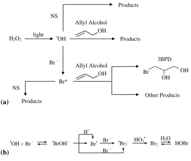
In this method X*(aq) species (where X=Br or Cl) react with allyl alcohol to form halogenated diols that are then quan-tified. We chose allyl alcohol (AA) as the probe because: i) it has a relatively high water solubility; ii) the double bond serves as the site of reaction for X*(aq), leading to the formation of stable halogenated products that are com-mercially available; iii) a number of rate constants for reac-tions of X*(aq) with AA have been reported; and v) AA does not absorb wavelengths of light present in the troposphere (i.e., above 290 nm). Chemistry in our experiments is ini-tiated by photolysis of hydrogen peroxide (H2O2), forming •OH that oxidizes Br−to form Br*(aq), which in turn adds
to AA to form 3-bromo-1,2-propanediol (3BPD) (Fig. 1a). Figure 1b illustrates the major reactions that form the reac-tive bromide species (Br*(aq)) in our experiments. While Br•, Br2, and HOBr are the dominant sources of 3BPD under
our conditions, their relative contributions depend upon their steady-state concentrations, which depend upon experimen-tal parameters such as pH, [Br−], and [AA]. Finally, while our technique can determine reactive bromide and chloride species, it is not currently suitable for iodine because iodi-nated diols are extremely unstable in aqueous solution.
We developed this reactive halogen technique by first per-forming a series of increasingly complex experiments and
using the results to build and test a kinetic model of the•
OH-initiated oxidation of bromide in the presence of our probe. In these experiments we varied several different parameters (pH, [Br−], and [AA]) while measuring three endpoints: i) the steady-state concentration of hydroxyl radical ([•OH]), ii) the rate of allyl alcohol loss (RLAA), and iii) the rate of 3BPD formation (R3BPDF ). We then used the kinetic model developed from these experiments to evaluate the overall chemical probe technique, and a series of three data treat-ments, under a range of experimental conditions.
2.2 Experimental conditions and techniques
2.2.1 General experimental parameters
NaBr (99.99%) and H2SO4(Optima) were from Aldrich and
Fisher, respectively; all other reagents were A.C.S. reagent grade or better. Type I reagent grade water (≥18.2 M-cm) was obtained from a Millipore Milli-Q Plus system. Illumi-nation solutions contained 1.0 mM H2O2(Fisher) as a
photo-chemical source of•OH (and HO•2via the•OH+H2O2
reac-tion); H2O2stock concentrations were verified daily by UV
absorbance (ε240=38.1 M−1cm−1; Miller and Kester, 1988).
Sample pH values were adjusted using 1.0 M H2SO4(for pH
≤5.5) or a solution of 1.0 mM sodium tetraborate and 0.30 M NaOH (pH>5.5). Based on control experiments where only sodium hydroxide was used to adjust the pH, the presence of borate had no effect on chemistry in our solutions.
Samples (∼23 mL) were air-saturated and were illumi-nated with 313 nm light from a 1000 W Hg/Xe monochro-matic system (Arakaki et al., 1995) in closed 5 cm quartz cells (FUV quartz, Spectrocell) that were stirred continu-ously and maintained at 20◦C. Over the course of
illumina-tion (typically 1 h), aliquots of sample were removed at spec-ified times (every ∼10–15 min) and analyzed for•OH, AA,
or 3BPD; a total of <15% of the initial volume of sample was removed during any experiment. In order to calculate pho-tolysis rates the actinic flux was measured during each ex-periment using 2-nitrobenzaldehyde actinometry (Anastasio et al., 1994). Illuminated controls showed that there was no loss of AA and no formation of 3BPD in samples that did not contain H2O2, regardless of whether bromide was present.
Separate experiments on solutions containing 1.0 mM H2O2,
0.80 mM Br−, and 3BPD showed that there was no loss of 3BPD during illumination. Dark controls were prepared by placing ∼4 mL of sample in a 1 cm airtight quartz cell, plac-ing it in a dark cell chamber (20◦C, stirred), and taking a sample at the final illumination time point. Rates of 3BPD formation in the dark controls were generally negligible and were subtracted from the corresponding illuminated rates.
2.2.2 Measurements of•OH, allyl alcohol, and 3BPD
The rate of formation, lifetime, and steady-state concen-tration of •OH were measured using the formation of
m-hydroxybenzoic acid (m-HBA) from the reaction of•OH
with a benzoic acid (BA) chemical probe (Zhou and Mop-per, 1990). m-HBA was measured on an isocratic high-pressure liquid chromatographic (HPLC) system consisting of a Shimadzu LC10-AT pump and SPD-10AV UV/Vis de-tector with a Keystone Scientific C-18 Beta Basic reverse-phase column (250×3 mm, 5 µm bead) and guard column (Anastasio and McGregor, 2001). Allyl alcohol loss was measured on the same HPLC system using an eluent of 5% acetonitrile/95% H2O at a flow rate of 0.60 mL min−1
and a detection wavelength of 200 nm. Concentrations of AA were determined based on calibration standards made in Milli-Q water run during the day of an experiment; the addition of Br−had no significant effect on AA quantifica-tion. Calibration curves were very linear (with R2 values typically >0.99) and values for replicate injections gener-ally agreed within 5%. We did not determine a detection limit for the AA technique, but we could readily measure concentrations near 2 µM in our laboratory solutions. 3-bromo-1,2-propanediol (3BPD) was extracted and analyzed by GC-ECD as detailed previously (Matthew and Anasta-sio, 2000) with minor changes as described in the supple-mentary material (http://www.atmos-chem-phys.net/6/2423/ 2006/acp-6-2423-2006-supplement.pdf; Sect. S.1; note that section, equation or table numbers with the prefix “S” are all supplementary material).
The rate of 3BPD formation in a given experiment was determined as the slope of a linear regression in a plot of [3BPD] versus illumination time. (The same procedure is used for determining formation rates for the chlorinated diol in Part 2.) The rate of loss of allyl alcohol in a given ex-periment (i.e., at a given initial AA concentration) was deter-mined by first taking a linear regression of ln([AA]t/[AA]0)
versus illumination time, where [AA]t is the concentration
at time t and [AA]0is the initial concentration in the
exper-iment. The slope of this plot is the negative of the pseudo first-order rate constant for AA loss. We multiplied this rate constant by [AA]0to determine the initial rate of AA loss for
each solution.
2.2.3 Kinetic models
The program Acuchem (Braun et al., 1988) was used to model aqueous halide radical chemistry in the illuminated solutions. The complete kinetic model used here (“Br−Full
Model”) is composed of 87 reactions that describe the pho-tolysis of H2O2to form hydroxyl radical and the subsequent •OH-initiated reactions with bromide and allyl alcohol as
outlined in Figs. 1a and b. All of the reactions in the model are described in Tables S1–S3. For a given model run the pH was fixed at the experimentally measured value. One key pa-rameter that we used to fit the model to the experimental data was the set of reactions of reactive bromine species (Br*(aq)) with AA to form 3BPD and other products:
Br∗(aq) + AA → 3BPD (R1) (a) H2O2 light • OH NS Products Products Br – Br* Other Products NS Products Br 3BPD OH OH Allyl Alcohol OH Allyl Alcohol OH (b) • BrOH– H+ Br• Br – HO 2• HOBr • OH + Br – H2O Br2 • Br2– Br –
Fig. 1. (a) Simplified scheme showing the formation of reactive
bromine species (Br*) and their reaction with allyl alcohol (AA) to form 3-bromo-1,2-propanediol (3BPD). Note that AA also con-sumes•OH, thereby decreasing the rates of formation of Br*(aq) and 3BPD (i.e., the “AA effect”). NS=natural scavengers, i.e., all other sinks (including H2O2) for•OH and Br*(aq). (b) An
overview of the major reactions that form reactive bromine species (Br*) in our solutions. Note that the reactions are not balanced; see the supplementary material (http://www.atmos-chem-phys.net/ 6/2423/2006/acp-6-2423-2006-supplement.pdf; Tables S1–S3) for a complete list of the balanced reactions.
Br∗(aq) + AA → other products (R2)
While the total rate constant (i.e., kR1+kR2)for reaction of a
given Br*(aq) species with AA was fixed based on literature data, we chose the relative sizes of kR1 and kR2 to fit the
experimental data. In this way we determined Yi3BPD, the yield of 3BPD from the reaction of Br*(aq) species i with AA:
Yi3BPD= kR1
kR1+kR2
(1)
Rate constants for each Br*(aq) species with AA, and the corresponding yields of 3BPD, are listed in Table S3 of the supplementary material (http://www.atmos-chem-phys. net/6/2423/2006/acp-6-2423-2006-supplement.pdf).
2.3 Overview of competition kinetics
Performing competition kinetics experiments with a chem-ical probe allows quantitative determination of the steady-state concentration ([i]), rate of formation (RiF), and lifetime (τi)of a reactive species i. Although experiments are
con-ducted in the presence of varying concentrations of the probe compound, the values for [i], RFi and τi obtained from the
0 20 40 60 80 100 0.00 0.02 0.04 0.06 0.08 0.10
Inverse of Allyl Alcohol Concentration (106 M-1)
Inv e rse of 3 BPD Fo rmati o n Rate (1 0 9 s M -1 ) Full Model Model with No OH + AA
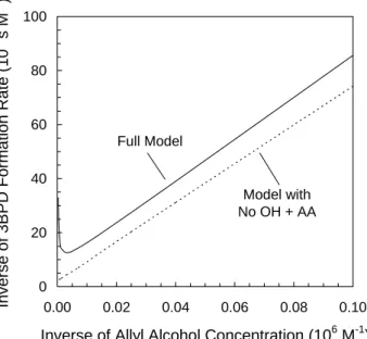
Fig. 2. Inverse plots for 1/R3BPDF,tot from data generated from two
different models under the same conditions (0.80 mM Br−, 10– 1000 µM AA, pH 5.3). The solid line was generated from the “Br− Full Model” and illustrates the nonlinear behaviour associated with increasing [AA] (i.e., decreasing 1/[AA]). The dashed line was gen-erated from the “No•OH+AA Model”, which is identical to the Br−Full Model except that AA is not allowed to react with•OH. The difference in the two lines illustrates the impact of the “AA effect”.
[probe]=0). For example,•OH kinetics in solution can be measured by determining the rate of m-HBA formation from the reaction of •OH with added benzoic acid (BA) (Zhou
and Mopper, 1990; Anastasio and McGregor, 2001). Plot-ting the inverse of the rate of m-HBA formation as a function of the inverse of the BA concentration (i.e., making an “in-verse plot”) produces a straight line; the slope and y-intercept of this line are then used to calculate [•OH], RFOH, and τOH.
A key feature of this technique is that the addition of BA does not affect the rate of•OH formation and, therefore, the inverse plot is linear over the entire [BA] range.
In contrast, in the technique described here the formation rate of the reactive bromine species (Br*(aq)) is affected by the addition of the probe compound, allyl alcohol (AA). As shown in Fig. 1a, in the absence of allyl alcohol •OH
re-acts with either natural scavengers (NS) or with Br−to form
Br*(aq). AA added to the solution reacts with Br*(aq) to form 3BPD, but it is also a sink for•OH, which lowers the steady-state•OH concentration and therefore lowers the rate of Br*(aq) formation. As long as Br−is the dominant sink for•OH, the decrease in the rate of Br*(aq) formation due to AA addition is relatively small, and the rate of formation of 3BPD (RF3BPD) rises with increasing AA concentrations. However, once AA becomes the dominant sink for•OH, the
formation rates of Br*(aq) and 3BPD both decrease substan-tially.
This “AA effect” has two major impacts on the “inverse plot” from the AA competition kinetics experiment (i.e., 1/RF3BPD vs. 1/[AA]). As illustrated in Fig. 2, the first ef-fect is that at high AA concentrations, the probe becomes the dominant sink for•OH and the rate of 3BPD formation slows dramatically, resulting in a quick increase in 1/RF3BPD (i.e., the plot is non-linear at high [AA]). The second effect is more subtle, but also important. Even though the inverse plot may not be linear over the entire range of 1/[AA], the data are linear at low values of [AA] (i.e., high values of 1/[AA]) where AA is a minor sink for•OH. However, even
within this linear range, the presence of AA decreases the rate of Br*(aq) formation, changing the slope and y-intercept of the inverse plot from what they would be if•OH did not react with AA (Fig. 2). For the pH and [Br−] values used for our experiments, the effect on the slope is very small but the effect on the y-intercept can, under certain conditions, be large enough to considerably bias the experimental results. However, as discussed below, in many cases corrections can be made for these biases.
While in theory the relationship between the rate of 3BPD formation from all Br*(aq) species and the concentration of added AA can be derived mathematically from the series of elementary reactions that describe the experimental system, in practice this can be extremely difficult. As described in the supplementary material (http://www.atmos-chem-phys.net/ 6/2423/2006/acp-6-2423-2006-supplement.pdf; Sect. S.2), we can derive this equation for Br• in the case where this radical is the dominant source of 3BPD:
1 RF,3BPDtot =a + b [AA]+c[AA] (S13) a = (k AA OH k 0NS Br + kBrAAk 0NS OH) FBr3BPD RBrF YBr3BPDkAABr k0NS OH (S14) b = F 3BPD Br YBr3BPDkBrAA[Br•] (S15) c = k AA OH F 3BPD Br RFOHYBr3BPDkOHBr−[Br−]YOHBr = k AA OH F 3BPD Br k0NS OH YBr3BPDRFBr (S16)
where R3BPDF,tot is the total rate of 3BPD formation from all species, FBr3BPDis the fraction of 3BPD that is formed from the reaction of Br•with AA (Sect. S.4), YBr3BPD is the yield of 3BPD from the reaction of Br•with AA (Eq. 1), and knm is the rate constant for the reaction of species m with n. The variables a, b, and c are determined by fitting the experimen-tal data (RF,3BPDtot as a function of [AA]) to Eq. (S13) using a nonlinear least-squares technique (Sigmaplot, version 4.0).
By rearranging the b and c terms it is possible to solve for [Br•], RBr F , and τBr: [Br•] = F 3BPD Br b YBr3BPDkAABr (S17) RFBr= k AA OH F 3BPD Br c k0NS OHYBr3BPD (S18) τBr= c k0NSOH b kOHAAkAABr = [Br•] RBrF (S19)
These Br• kinetic terms are determined by using the non-linear least squares fitted values for a, b, and c in conjunction with FBr3BPD, YBr3BPD, and kmn.
Because this kinetic derivation takes into account the ef-fect of AA on [•OH] and the formation of Br•, Eq. (S13)
accounts for the “AA effect”. Although similar expressions can be derived for Br2 and HOBr, these expressions
con-tain several terms that are currently unknown and that are hard to estimate (e.g., the formation rate and concentration of HO•2; Sect. S.2). Because of these unknown parameters, using equations analogous to Eq. (S13) to determine the Br2
and HOBr kinetics is currently not feasible.
However, the kinetics of Br2and HOBr can be measured
by working in the linear range of the 1/R3BPDF,totversus 1/[AA] plot where AA concentrations are low (Fig. 2). In this linear range, we assume that the low AA concentrations have little effect on [•OH] and on the rates of Br*(aq) and 3BPD forma-tion (i.e., the AA effect is minimized). In this case Eq. (S13) can be simplified to (Sect. S.3):
1
RF,t ot3BPD
=a0 + b
0
[AA] (S25)
where a0 and b0 are the y-intercept and slope of the linear portion of the inverse plot, respectively:
a0= F 3BPD i Yi3BPDRiF (S26) b0= F 3BPD i Yi3BPDkiAA[i] (S27)
The a0 and b0 terms can be rearranged to solve for [i], Ri F, and τias follows: [i] = F 3BPD i b0Y3BPD i kiAA (S28) RFi = F 3BPD i a0Y3BPD i (S29) τi = a0 b0 kAA i = [i] RiF (S30)
These equations are applicable for any Br*(aq) species i (e.g., Br•, Br
2, and HOBr) and are analogous to those
de-rived for the•OH system with BA as the probe (Zhou and
Mopper, 1990; Anastasio and McGregor, 2001).
Using the linear Eq. (S25) instead of the more complex Eq. (S13) implicitly assumes that AA has only a minor effect upon•OH (and, therefore on Br*(aq) and 3BPD formation) in the linear portion of the inverse plot. The advantage of this assumption is that it allows Eq. (S25) to be broadly applied to all reactive Br*(aq) species i (Sect. S.3). The disadvantage is that, while it generally has a minor effect on the determi-nation of [i], it can introduce large (though often correctable) errors in the determination of RFi and τi.
3 Results and discussion
3.1 Experiments with only hydrogen peroxide and allyl al-cohol
As a first step in examining the probe chemistry, we il-luminated pH 5.5 solutions containing 1.0 mM H2O2 with
and without AA to test whether we could correctly model
•OH steady-state concentrations. In a 1.0 mM H 2O2
so-lution, the experimentally measured [•OH] (±1 SE) was (2.1±0.1)×10−13M, in good agreement with the model value of 2.8×10⁻¹³M (the relative percent difference (RPD) between these values is 29%). When 75 µM of allyl alco-hol was added to a 1.0 mM H2O2 solution, the measured
value for [•OH] (±1 SE) dropped to (1.3±0.1)×10−14M, in good agreement with the modeled value of 1.7×10⁻¹⁴M (RPD=27%).
In the second set of experiments, we measured the rate of loss of AA (RAAL ) in pH 5.5 solutions containing 1.0 mM H2O2 and 15–1000 µM allyl alcohol. As seen in Fig. 3,
RLAA increases rapidly between 15 and 150 µM AA but is relatively constant at higher concentrations where AA is the dominant sink for•OH. Modeled rates of loss are within the experimental errors of the measured values out to 300 µM AA, but are overpredicted at higher [AA]. An additional ex-periment performed at pH 3.0 (75 µM AA) gave nearly iden-tical results to the pH 5.5 experiment and was in good agree-ment with the model (RPD=3%, Fig. 3).
There are two mechanisms for AA loss in our model: di-rect reaction between AA and oxidants (e.g., •OH, Reac-tion 70, Table S3) and polymerizaReac-tion reacReac-tions involving AA radicals (formed from the reaction of•OH or Br* with
AA) and another molecule of AA (e.g., Reactions 71–73, Table S3). Comparing the calculated rate of •OH forma-tion in these experiments (0.43 µM min−1) with the mea-sured rate of AA loss in the plateau of Fig. 3 (0.69 µM min−1), indicates that approximately 40% of AA loss is due to polymerization reactions in this region. Although poly-merization during free-radical additions is well established (March, 1992), we were unable to find rate constants for the
0.0 0.2 0.4 0.6 0.8 1.0 0 200 400 600 800 1000
Concentration of Allyl Alcohol (μM)
Rate of AA Loss (μ M min -1 ) Experiment, pH 5.5 Experiment, pH 3.0 Model, pH 5.5
Fig. 3. Rate of allyl alcohol loss (RAAL )as a function of [AA] in
illuminated (313 nm) aqueous solutions (pH 5.5) containing only AA and 1.0 mM H2O2. The open diamonds are experimental values
with error bars representing 90% confidence intervals (CI), based on the standard error of the slope from a plot of AA loss at each [AA]. The line is the model result using the Br−Full Model with [Br−]=0. The filled diamond at 75 µM AA is the measured rate of AA loss at pH 3.0.
polymerization of aqueous AA. The good agreement in the modeled and measured values for AA loss at lower AA con-centrations indicate that our modeled rate constants for poly-merization are reasonable at most of the AA concentrations we employed, but not at the higher concentrations. As shown later, this overestimate of allyl alcohol loss at high [AA] does not affect the model predictions of 3BPD formation or the calculated Br*(aq) kinetics.
3.2 •OH measurements in the presence of bromide
To begin to test and constrain the kinetic model in bromide solutions we first measured the•OH steady-state concentra-tion in illuminated soluconcentra-tions (1.0 mM H2O2, pH 5.5)
con-taining seawater levels of bromide (0.80 mM; Zafiriou et al., 1987) with and without allyl alcohol. In the absence of AA, the measured and modeled values of [•OH] were nearly iden-tical (7.1±0.2)×10−15 and 7.0×10⁻¹⁵M, respectively). In the presence of AA, the RPD between the measured and modeled values of [•OH] was <5% for experiments with 15, 40 and 75 µM AA and was 47% in a solution with 150 µM AA. Thus the model does a good to excellent job of repre-senting•OH chemistry in the presence of bromide.
0 10 20 30 2.0 3.0 4.0 5.0 6.0 7.0 8.0 9.0 pH R a te of 3B P D F o rm at io n ( n M m in -1 ) Experiment Model
(a)
0 50 100 150 200 250 2.0 3.0 4.0 5.0 6.0 7.0 8.0 9.0 pH Rat e of A A loss (nM min -1 ) Experiment Model(b)
Fig. 4. (a) Rate of 3-bromo-1,2-propanediol (3BPD) formation
(R3BPDF,tot) as a function of pH in illuminated (313 nm) aqueous bromide solutions ([Br−]=0.80 mM) containing 1.0 mM H2O2and
75 µM AA. The squares are experimental values of RF,tot3BPD. Error bars for 3BPD represent the 90% confidence interval for each point, calculated from the standard error of the slope from plots of 3BPD versus time at each pH. The line is the result from the “Br− Full Model”. (b) Rate of AA loss as a function of pH in the illuminated aqueous bromide solutions described in Fig. 4a. The symbols, line, and error bars are the same as in Fig. 3.
3.3 Formation of 3BPD (RF,3BPDtot)and loss of AA (RAAL )as a function of pH
To build and test our model as a function of pH, we con-ducted experiments on solutions containing 0.80 mM NaBr, 1.0 mM H2O2, and 75 µM AA over the pH range of 2.3 to
8.6. As shown in Figs. 4a and b, the model correctly de-scribes both RF,3BPDtot and RAAL over a wide range of pH. Of particular interest is the large increase in the rate of 3BPD formation at low pH (Fig. 4a), which is caused by the re-action of HO•2with•Br−2 to form Br2(Fig. 1b), which then
reacts with AA to form 3BPD (Matthew et al., 2003). In our experiments 3BPD is formed by Br•, Br2, and
HOBr, and the relative importance of each species as a source of 3BPD changes as a function of pH and other experimental conditions (Sect. S.4). Under the conditions of Fig. 4, Br2is
the most important species at low pH values (<4) while Br• is most important at higher pH values. The dibromide radical anion (•Br−2)and tribromide ion (Br−3)have concentrations that are in the same general range as Br•and Br2, but their
reactions with AA are too slow for them to contribute signifi-cantly to 3BPD formation (Reactions 80 and 86 in Table S3). In addition,•BrOH−(Fig. 1b) might also react with AA to form 3BPD, but this reaction appears to be unimportant un-der all of our experimental conditions and is therefore not included in the kinetic model.
Additional evidence that the model correctly describes aqueous bromide radical chemistry comes from a separate set of experiments conducted in the absence of AA that mea-sured the release of gaseous bromine (Br*(g), i.e., Br2 or
HOBr) from air-purged, illuminated solutions (0.10 M Br−, 1.0 mM H2O2, no AA) (Matthew et al., 2003). As described
in this previous paper, the release of Br*(g) occurs only dur-ing illumination, is strongly dependent on pH, and is very similar to the pH dependence of 3BPD (Fig. 4a). By setting [AA]=0, and adding reactions for the volatilization of Br*(g), the model is able to reproduce these experimental results.
3.4 Formation of 3BPD (RF,3BPDtot)and loss of AA (RLAA)as a function of [AA]
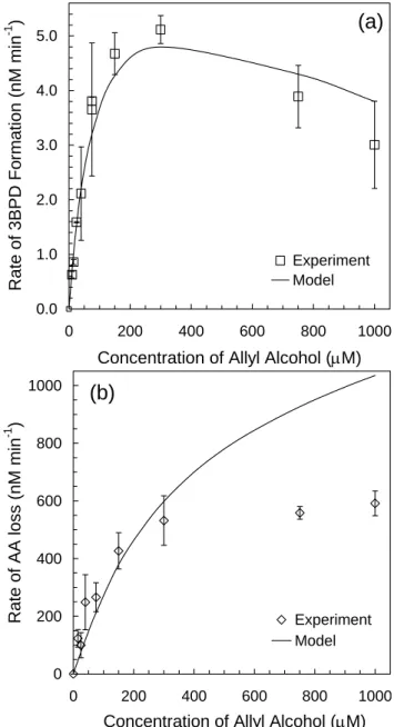
In the final set of five experiments, we measured RF,3BPDtot and
RLAA as a function of [AA] to test the model under condi-tions of pH and [Br−] that are representative of seawater and sea-salt particles (Table 1). As described in Sect. 3.7, these are also the competition kinetics experiments that we used as the final test of the probe technique. In the first exper-iment we used pH 5.3 solutions containing 0.80 mM NaBr, 0.91 mM H2O2and 10–1000 µM AA. As shown in Fig. 5a,
RF,3BPDtotincreases with [AA] up to ∼300 µM (due to increased scavenging of Br*(aq) by AA) but declines at higher AA con-centrations (because of AA reacting with•OH). The model
does a good job of explaining observed values of RF,3BPDtot as a function of [AA], with an average RPD between the model and experimental data of 11% (Table 1). Although Br•has the lowest steady-state concentration of the impor-tant Br*(aq) species, it is the dominant source of 3BPD in this experiment because of its rapid rate of reaction with AA (Table S3). As shown in Fig. 5b, measured rates of allyl alcohol loss increase with [AA] up to 300 µM and are es-sentially constant at higher [AA] where the probe scavenges
0.0 1.0 2.0 3.0 4.0 5.0 0 200 400 600 800 1000
Concentration of Allyl Alcohol (μM)
Rate of 3BPD F o rm ation (nM min -1 ) Experiment Model
(a)
0 200 400 600 800 1000 0 200 400 600 800 1000Concentration of Allyl Alcohol (μM)
R a te o f AA l o ss (n M mi n -1 ) Experiment Model
(b)
Fig. 5. (a) Experimental and model values of the total rate of
3-bromo-1,2-propanediol (3BPD) formation (R3BPDF,tot)for competition kinetics Experiment 1 (pH 5.3, 0.80 mM Br−, 1.0 mM H2O2, 10– 1000 µM AA, 313 nm illumination). Symbols, line, and error bars are the same as in Fig. 4a. (b) Experimental and model values of the rate of allyl alcohol loss (RLAA)as a function of allyl alcohol concentration for competition kinetics experiment 1 presented in Fig. 5a and Table 1. The symbols, line, and error bars are the same as described in Fig. 3.
most of•OH. The model matches allyl alcohol loss rates at the lower AA concentrations (<300 µM) but overestimates
RLAAat higher concentrations, as in the solutions containing only AA and H2O2(Fig. 3). As stated previously, this
Table 1. Parameters for competition kinetic experiments.
Exp # [Br
−
]
pH [AA] range tested Linear AA range
a Agreement between model
mM and experimentc(Average RPD)
µM nb µM nb RF,tot3BPD RAAL 1 0.80 5.3 10–1000 9 10–150 6 11 43 2 0.80 3.0 10–8000 11 10–110 5 41 41 3 0.40 5.4 10–3000 10 10–150 6 26 25 4 0.80 8.4 10–5000 8 10–75 5 38 40 5 8.0 5.3 75–500 3 75–500 3 8 14
The concentration of H2O2for all experiments was 0.91–1.0 mM. The photolysis rate constant for H2O2(jH2O2)was (3.8–4.0)×10−6s−1
for Experiments 1–3, 2.6×10⁻⁶s−1for Experiment 4, and 3.0×10⁻⁶s−1for Experiment 5.
aRange of allyl alcohol concentrations over which the inverse plot (1/R3BPD
F,tot vs. 1/[AA]) is linear. Note that the linear range can change
when the inverse plots are based on 3BPD formation rates from individual species, as is done in treatment C.
bNumber of points sampled within the specified range.
cAgreement between the experimental data and model output, calculated as the average of the absolute values of the RPD (relative percent
difference) between the model and experimental values of R3BPDF,tot(and RAAL )over the entire range of allyl alcohol concentrations. Note that the listed RPD value for RF,tot3BPDis the same as that for 1/R3BPDF,tot(and similarly for RLAAand 1/RAAL ).
simplified parameterization of radical-initiated AA polymer-ization, but this issue does not affect our halogen kinetics results.
The other four experiments in this series were conducted by varying [AA] in a set of identical solutions where each set had different values for pH and/or [Br−] (Table 1). As listed in the column of Fi3BPD values in Table 2 (see data treat-ment B), the relative contributions of Br•, Br2, and HOBr to
3BPD formation vary significantly throughout this set of ex-periments. Despite this, the model does a good to fair job of describing the rates of 3BPD formation and AA loss in these additional experiments, with the best agreement at pH
∼5. As shown in Table 1, the average RPD values between the measured and modeled values in Experiments 2–5 ranged from 8–41% for RF,3BPDtot and 14–41% for RAAL .
3.5 Competition kinetics: overview and expected values
Our kinetic model (the “Br− Full Model”) was built and constrained using the sets of experiments described above. The good agreement between the modeled and measured val-ues of [•OH], R3BPDF,tot and RLAA in these experiments gives us confidence that the model reasonably describes the• OH-mediated oxidation of bromide and subsequent reactions of Br*(aq) with allyl alcohol. In the next two sections (3.6 and 3.7) we use this model to test the ability of the allyl alco-hol chemical probe technique to measure reactive halogen species. This test consists of two major steps. In the first (Sect. 3.6), we examine the validity of the kinetic equations we derived for [i], RiF and τi (e.g., Eqs. S17–S19 and S28–
S30; Sect. 2.3) using “data” generated from simulated model experiments. In the second testing step (Sect. 3.7), we apply the same data treatments to actual data from laboratory
com-petition kinetics experiments in order to examine the overall utility of the probe technique for measuring [i], RiF and τi.
In order to examine whether our derived equations for [i],
RFi and τi give valid results, we first determined the
“ex-pected” values of these quantities for a given set of conditions (e.g., [Br−] and pH) using output from the model run under
these conditions. Expected values for steady-state concen-trations of Br•, Br2, and HOBr were obtained directly from
model runs performed under the same conditions as the cor-responding experiment except that AA concentrations were set to zero. (As described in Sect. 2.3, values derived from the competition kinetics analyses are for the case where no allyl alcohol is present.)
For each set of model conditions we also calculated the expected values for the rates of formation of Br*(aq). For Br•, its primary source (∼100%) is the reaction of•OH with Br−(Reaction 29, Table S2), and thus the expected rate of
formation (RFBr)in the absence of AA is:
RFBr=kOHBr−[•OH][Br−]YOHBr (2)
where kBr−OH is the rate constant for the reaction of•OH with Br−and YOHBr is the yield of Br•formed from the reaction of
•OH with Br−(Sect. S.5). Since molecular bromine (Br 2)
in our experiments originates primarily from the reaction of•Br−2 with hydroperoxyl radical (HO•2)(Reaction 45, Ta-ble S2), the rate of Br2formation (RBrF2)is calculated from:
RBr2 F =k HO2 Br−2 [HO • 2][ • Br−2] (3)
In the case of HOBr, we use the fact that it is at steady-state (as are the other Br*(aq)) and thus RFHOBris equal to the rate of HOBr destruction (RDHOBr), which can be more accurately
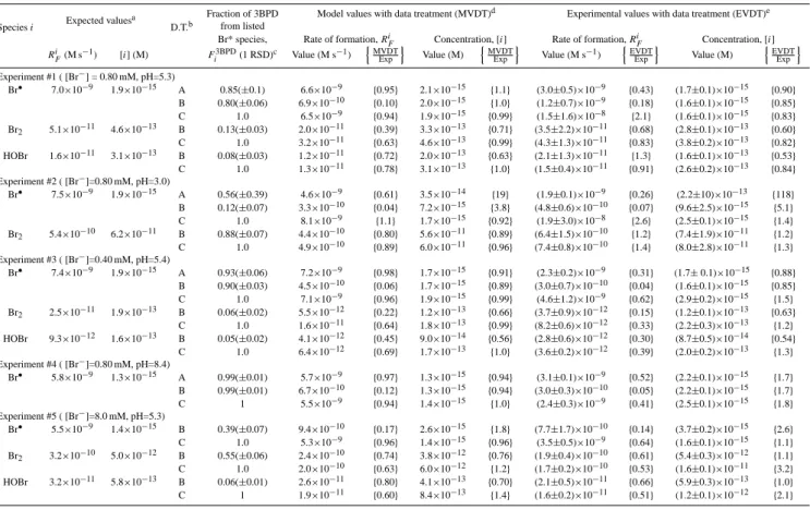
Table 2. Results of the kinetic analyses of the model and experimental data from the bromide competition kinetics experiments.
Species i Expected values
a
D.T.b
Fraction of 3BPD Model values with data treatment (MVDT)d Experimental values with data treatment (EVDT)e
from listed
Br* species, Rate of formation, Ri
F Concentration, [i] Rate of formation, RiF Concentration, [i]
Ri F(M s −1) [i] (M) F3BPD i (1 RSD)c Value (M s −1) n MVDT Exp o Value (M) nMVDT Exp o Value (M s−1) n EVDT Exp o Value (M) nEVDT Exp o Experiment #1 ( [Br−] = 0.80 mM, pH=5.3) Br• 7.0×10⁻⁹ 1.9×10⁻¹⁵ A 0.85(±0.1) 6.6×10⁻⁹ {0.95} 2.1×10⁻¹⁵ {1.1} (3.0±0.5)×10−9 {0.43} (1.7±0.1)×10−15 {0.90} B 0.80(±0.06) 6.9×10⁻¹⁰ {0.10} 2.0×10⁻¹⁵ {1.0} (1.2±0.7)×10−9 {0.18} (1.6±0.1)×10−15 {0.85} C 1.0 6.5×10⁻⁹ {0.94} 1.9×10⁻¹⁵ {0.99} (1.5±1.6)×10−8 {2.1} (1.6±0.1)×10−15 {0.83} Br2 5.1×10⁻¹¹ 4.6×10⁻¹³ B 0.13(±0.03) 2.0×10⁻¹¹ {0.39} 3.3×10⁻¹³ {0.71} (3.5±2.2)×10−11 {0.68} (2.8±0.1)×10−13 {0.60} C 1.0 3.2×10⁻¹¹ {0.63} 4.6×10⁻¹³ {0.99} (4.3±1.3)×10−11 {0.83} (3.8±0.2)×10−13 {0.82} HOBr 1.6×10⁻¹¹ 3.1×10⁻¹³ B 0.08(±0.03) 1.2×10⁻¹¹ {0.72} 2.0×10⁻¹³ {0.63} (2.1±1.3)×10−11 {1.3} (1.6±0.1)×10−13 {0.53} C 1.0 1.3×10⁻¹¹ {0.78} 3.1×10⁻¹³ {1.0} (1.5±0.4)×10−11 {0.91} (2.6±0.2)×10−13 {0.84} Experiment #2 ( [Br−]=0.80 mM, pH=3.0) Br• 7.5×10⁻⁹ 1.9×10⁻¹⁵ A 0.56(±0.39) 4.6×10⁻⁹ {0.61} 3.5×10⁻¹⁴ {19} (1.9±0.1)×10−9 {0.26} (2.2±10)×10−13 {118} B 0.12(±0.07) 3.3×10⁻¹⁰ {0.04} 7.2×10⁻¹⁵ {3.8} (4.8±0.6)×10−10 {0.07} (9.6±2.5)×10−15 {5.1} C 1.0 8.1×10⁻⁹ {1.1} 1.7×10⁻¹⁵ {0.92} (1.9±3.0)×10−8 {2.6} (2.5±0.1)×10−15 {1.4} Br2 5.4×10⁻¹⁰ 6.2×10⁻¹¹ B 0.88(±0.07) 4.4×10⁻¹⁰ {0.80} 5.6×10⁻¹¹ {0.89} (6.4±1.5)×10−10 {1.2} (7.4±1.9)×10−11 {1.2} C 1.0 4.9×10⁻¹⁰ {0.89} 6.0×10⁻¹¹ {0.96} (7.4±0.8)×10−10 {1.4} (8.0±2.8)×10−11 {1.3} Experiment #3 ( [Br−]=0.40 mM, pH=5.4) Br• 7.4×10⁻⁹ 1.9×10⁻¹⁵ A 0.93(±0.06) 7.2×10⁻⁹ {0.98} 1.7×10⁻¹⁵ {0.91} (2.3±0.2)×10−9 {0.31} (1.7± 0.1)×10−15 {0.88} B 0.90(±0.03) 4.5×10⁻¹⁰ {0.06} 1.7×10⁻¹⁵ {0.89} (3.0±0.7)×10−10 {0.04} (1.6±0.1)×10−15 {0.85} C 1.0 7.1×10⁻⁹ {0.96} 1.9×10⁻¹⁵ {0.99} (4.6±1.2)×10−9 {0.62} (2.9±0.2)×10−15 {1.5} Br2 2.5×10⁻¹¹ 1.9×10⁻¹³ B 0.06(±0.02) 5.5×10⁻¹² {0.22} 1.2×10⁻¹³ {0.66} (3.7±0.9)×10−12 {0.15} (1.2±0.1)×10−13 {0.63} C 1.0 1.6×10⁻¹¹ {0.64} 1.8×10⁻¹³ {0.99} (8.2±0.6)×10−12 {0.33} (2.2±0.3)×10−13 {1.2} HOBr 9.3×10⁻¹² 1.6×10⁻¹³ B 0.05(±0.02) 4.1×10⁻¹² {0.45} 9.0×10⁻¹⁴ {0.56} (2.8±0.6)×10−12 {0.30} (8.7±0.5)×10−14 {0.54} C 1.0 6.4×10⁻¹² {0.69} 1.7×10⁻¹³ {1.0} (3.6±0.2)×10−12 {0.39} (2.0±0.2)×10−13 {1.3} Experiment #4 ( [Br−]=0.80 mM, pH=8.4) Br• 5.8×10⁻⁹ 1.3×10⁻¹⁵ A 0.99(±0.01) 5.7×10⁻⁹ {0.97} 1.3×10⁻¹⁵ {0.94} (3.1±0.1)×10−9 {0.52} (2.2±0.1)×10−15 {1.7} B 0.99(±0.01) 6.7×10⁻¹⁰ {0.12} 1.3×10⁻¹⁵ {0.94} (3.0±0.3)×10−10 {0.05} (2.2±0.1)×10−15 {1.7} C 1 5.5×10⁻⁹ {0.94} 1.4×10⁻¹⁵ {1.0} (2.4±0.3)×10−9 {0.41} (2.5±0.1)×10−15 {1.8} Experiment #5 ( [Br−]=8.0 mM, pH=5.3) Br• 5.5×10⁻⁹ 1.4×10⁻¹⁵ B 0.39(±0.07) 9.4×10⁻¹⁰ {0.17} 2.6×10⁻¹⁵ {1.8} (7.7±1.7)×10−10 {0.14} (3.7±0.2)×10−15 {2.6} C 1.0 5.3×10⁻⁹ {0.96} 1.4×10⁻¹⁵ {0.96} (3.5±0.5)×10−9 {0.64} (1.6±0.1)×10−15 {1.1} Br2 3.2×10⁻¹⁰ 5.0×10⁻¹² B 0.55(±0.06) 2.4×10⁻¹⁰ {0.74} 3.8×10⁻¹² {0.76} (1.9±0.4)×10−10 {0.61} (5.4±0.3)×10−12 {1.1} C 1.0 2.0×10⁻¹⁰ {0.63} 6.0×10⁻¹² {1.2} (1.7±0.2)×10−10 {0.53} (1.6±0.1)×10−11 {3.2} HOBr 3.2×10⁻¹¹ 5.8×10⁻¹³ B 0.06(±0.01) 2.6×10⁻¹¹ {0.80} 4.1×10⁻¹³ {0.70} (2.1±0.5)×10−11 {0.66} (5.9±0.3)×10−13 {1.0} C 1 1.9×10⁻¹¹ {0.60} 8.4×10⁻¹³ {1.4} (1.6±0.2)×10−11 {0.51} (1.2±0.1)×10−12 {2.1}
Lifetimes (τi)are not included in the table but can be calculated as τi=[i]
.
RiF. Similarly, values of MVDT/Exp for τi are calculated
by dividing the value of MVDT/Exp for [i] by the MVDT/Exp value for RiF. Values for EVDT/Exp for τi are calculated in an analogous
manner.
aExpected values are model-derived best estimates of the actual values for [i] and Ri
F in the experimental solutions in the absence of AA
(Sect. 3.5).
bData treatments (D.T.) are discussed in Sects. 3.6 and 3.7. Data treatment A, which works only for Br•
, uses all data in the inverse plot and accounts for the AA effect. Data treatments B and C use data in the linear range of the inverse plot with either a rough correction for the
Fi3BPDeffect (treatment B) or corrections for both the AA and Fi3BPDeffects (treatment C).
cAverage (±1 relative standard deviation) of F3BPD
i calculated over either the linear [AA] range (Table 1) for treatments B and C, or the
entire [AA] range for treatment A. Values for data treatment C are listed as 1.0 since in this case a separate inverse plot is made for each individual Br* species.
dCalculated by taking the model-derived results through the data treatment steps (Sect. 3.6).
eCalculated by taking the experimental results through the data treatment steps (Sect. 3.7). Errors are ±1 standard error calculated based on
the standard errors of the slope and y-intercept from the inverse plots.
calculated. Since H2O2accounts for >99% of HOBr loss in
our experiments
RFHOBr=RHOBrD =kH2O2
HOBr[H2O2][HOBr] (4)
Values of [•OH], [HO•2], [•Br−2], [H2O2], and [HOBr] in
Eqs. (2–4) are taken directly from the model. Expected val-ues for [i] and RFi under our range of experimental condi-tions are shown in Table 2. Expected values for τi are not
included in Table 2, but can be calculated as [i]/RFi .
3.6 Competition kinetics: model experiments and data treatments
As described above, the goal in this first step of technique testing is to examine the accuracy of the derived equations (and their accompanying assumptions) for determining [i],
RFi , and τi. To do this we use “data” generated from models
run using the conditions of the competition kinetic experi-ments (e.g., pH, Br−and [AA]; Table 1). The output from these “model experiments” (RF,3BPDtot as a function of [AA]) is
then used to generate inverse plots and calculate values of [i],
RFi , and τi using one of three different data treatments (A, B,
and C). The resulting values (referred to as “model values ob-tained with data treatments” or MVDT) are then compared to the expected values obtained from the model (Sect. 3.5).
3.6.1 Data treatment A
In the first data treatment we fit a curve to the entire set of inverse plot data (1/R3BPDF,totvs. 1/[AA]) using Eq. (S13) in or-der to obtain values for a, b, and c. Values of [i], RFi , and
τi are then calculated using Eqs. (S17–S19). Although this
technique can only be used for Br•(Sect. 2.3), its advantage is that Eq. (S13) takes into account the effects that AA has on [•OH] and, therefore, on RiF and RF,3BPDtot. Data treatment A was evaluated for Experiments 1–4 by using the Br−Full Model with the experimental conditions listed in Table 1. It could not be applied to Experiment 5 because the inverse plot is linear over the entire AA range, precluding us from deter-mining an accurate value for c. As with subsequent treat-ments, the validity of treatment A was evaluated by examin-ing the ratio of the model value to the expected value; these ratios (MVDT/Exp) are shown in Table 2.
Based on these results, data treatment A gives MVDT val-ues for [Br•] and RFBrthat are within 10% of expected values when Br•is the dominant source of 3BPD at all AA concen-trations (e.g., in Experiments 1, 3, and 4, where the average value for FBr3BPDin a given experiment is ≥0.85). It is im-portant to note that FBr3BPD used in these calculations is the average value over the entire 1/[AA] range, calculated based on data obtained from the Br−Full Model. The small
devia-tions between the MVDT and expected values are apparently a result of the error associated with this averaging. In cases where FBr3BPDis not large throughout the range of [AA], data treatment A does not perform well. For example, in Exper-iment 2 (pH 3.0, FBr3BPD(±1 RSD)=0.56±0.39) the MVDT value for RBrF is within a factor of 2 of the expected value, but [Br•] is overestimated by 19 times (Table 2) and τBr is
too large by ∼30 times (not shown).
3.6.2 Data treatment B
The second data treatment involves fitting a line to the lin-ear portion of the inverse plot using Eq. (S25) with a value of Fi3BPD from the Br− Full Model, where Fi3BPD here is the fraction of 3BPD from i averaged throughout the linear range of the inverse plot. The slope and y-intercept from the linear regression to the inverse plot data (1/RF,3BPDtot ver-sus 1/[AA]) are then used in Eqs. (S28–S30) to calculate [i],
RFi , and τi. As seen in Table 2, with one exception (Br•
in Experiment 2), this simple analysis generates MVDT val-ues of [i] for all species that are within a factor of 2 of the expected values. This is true even for species that are only minor sources of 3BPD (e.g., HOBr in Experiments 1, 3, and 5 where FHOBr3BPD≤0.08). In addition, MVDT values of RiF
obtained for Br2and HOBr using treatment B are nearly all
within a factor of 3 of the expected values. However, for reasons that are unclear, values of RFi for Br•are
underesti-mated by factors of 6 to 25 times using treatment B (Table 2). Errors in τi vary significantly and reflect the combination of
errors associated with RFi and [i].
3.6.3 Data treatment C
Like treatment B, treatment C is based on applying Eq. (S25) to the linear portion of the inverse plot. However, in treat-ment C more effort is taken to correct the data for the two possible biases associated with the competition kinet-ics derivations. The first bias is the “AA effect”, where the presence of AA reduces the formation rates of Br*(aq) and 3BPD. This bias appears because the kinetic equations for the linear portion of the inverse plot (e.g., Eq. S25) assume that the presence of low AA concentrations does not signifi-cantly affect RFi or R3BPDF,tot (Sect. 2.3). The second bias, the “Fi3BPDeffect”, arises from the fact that three species (i=Br•,
Br2, and HOBr) are responsible for different fractions of the
3BPD formed (i.e., Fi3BPD, Sect. S.4) and these contributions can vary with [AA].
To correct for these possible biases in the model “data” us-ing data treatment C, we first run a model that is identical to the Br−Full Model except that•OH is not allowed to react with AA. This “No •OH+AA Model” is run under the de-sired experimental conditions (e.g., Table 1) and at each AA concentration used in the model R3BPDF,tot is recorded and the value of Fi3BPDis determined (Eq. S31). From these data we calculate RF, i3BPD, the rate of 3BPD formation from an indi-vidual reactive bromine species i (i=Br•, Br2, and HOBr) at
each [AA]:
RF, i3BPD=RF,3BPDtot×Fi3BPD (5)
The next step is to use these data to generate inverse plots for each species (i.e., 1/RF, i3BPDas a function of 1/[AA]). The re-sulting inverse plots have been corrected for both the Fi3BPD and AA effects. The slope and y-intercept from the inverse plots are then used in Eqs. (S28) and (S29) to evaluate data treatment C. In contrast to treatments A and B, Fi3BPD for treatment C is set to 1 for each species because each in-verse plot represents 3BPD formation from only one Br*(aq) species. This correction for Fi3BPDin treatment C is more ac-curate than that used in treatments A and B since it accounts for the fact that Fi3BPDcan vary with [AA].
As seen in Table 2, MVDT values obtained through treat-ment C agree very well with the expected values for [i] and
RFi . The [i] values obtained for all three species from this treatment are typically within 10%, and always within 40%, of the expected values while values of RFi are within 10–40% of the expected values. Furthermore, those species with the largest discrepancies in RFi account for only a small fraction, typically <10%, of the 3BPD formed (e.g., Br2 in
quite good: typically within 15% of the expected value and always within a factor of 2.4.
3.6.4 Summary of data treatments with model-derived “data”
Overall, data treatment A, which can only be used to deter-mine Br•kinetics (Sect. 2.3), works very well for determin-ing values of [Br•], RFBr, and τBrunder conditions where Br•
is the dominant source of 3BPD at all [AA] values used in the experiment (Table 1). With one exception ([Br2] in
experi-ment 3), treatexperi-ment B provides good values (within a factor of ≈2 of expected values) of [i] and RFi for Br2and HOBr
under our experimental conditions. This treatment also pro-vides excellent results for [Br•] when Br• is the dominant source of 3BPD, but always significantly underpredicts RFBr (Table 2) and does not consistently give reliable results for τi
for any Br*(aq). The more complicated treatment C consis-tently provides the best results for all species under all con-ditions: i) values of [i] are within 10% of expected values except in two cases (within 20–40% for Br2 and HOBr in
Experiment 5), ii) rates of formation (RFi )are within 10% of expected values for Br•, and within 11–40% for Br2and
HOBr, and iii) lifetimes (τi)are within 15% of expected
val-ues for Br•and within a factor of 1.1–2.4 for Br2and HOBr.
3.7 Competition kinetics: experimental data and determi-nation of [i], RFi , and τi
3.7.1 Overview and procedures
Based on the model-derived results above, the kinetic equa-tions we derived to determine [i], RFi , and τi are generally
valid, although in some cases corrections are needed to ac-count for the AA and Fi3BPD effects. In this section we perform the second testing step: evaluating the probe tech-nique using experimental data. To do this we analyze the data from the laboratory experiments using the three different data treatments in order to determine the kinetics of Br*(aq) un-der different experimental conditions. The values obtained from this treatment of the experimental data are referred to as EVDT values (experimental values with data treatment). We then compare these EVDT values with the model-derived expected values (Sect. 3.5) to determine the reliability of the probe technique.
For data treatments A and B, values of [i], RFi , and τi
from the experimental data are calculated as described for the model data (Sects. 3.6.1 and 3.6.2), but for data treatment C the steps are slightly different in order to correct for both the Fi3BPDand AA effects. In the first step we separately run the Br−Full Model and the No•OH+AA Model (Sect. 3.6.3) with the desired experimental conditions (Table 1). For both models, RF,3BPDtot is recorded and Fi3BPDis calculated for each [AA]. We then calculate R3BPDF, i (Eq. 5) for each species i at every [AA] for both models and use the data to generate
in-verse plots for each species. The RF, i3BPDinverse plots from the Br− Full Model have been corrected for the Fi3BPD ef-fect, while those from the No•OH+AA Model have been corrected for both the Fi3BPDand AA effects. Thus differ-ences in the corresponding slopes (and y-intercepts) between the two sets of model data should be due to the AA effect. In the next step of treatment C we use these differences to calculate correction factors for the slope (b0)and y-intercept
(a0)for each i (Cb0 i and C a0 i , respectively): Cib0 = b 0 i(No OH + AA Model) b0 i(Br−Full Model) (6) Cia0 = a 0 i(No OH + AA Model) a0 i(Br−Full Model) (7)
where b0i and ai0 are the slope and y-intercept, respectively, from the linear regression to the inverse plot for each species generated from the specified model data (“Br−Full” or “No
•OH+AA”). Equations (S28–S30) can now be rewritten as
follows: [i] = 1 b0i Yi3BPDkAAi Cib0 (8) RFi = 1 ai0Yi3BPDCai 0 (9) τi = a0i Cia0 b0i kAAi Cib0 = [i] RiF (10)
The values of [i], RiF, and τi obtained with these equations
have been corrected for both the Fi3BPDand AA effects.
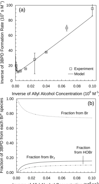
3.7.2 Kinetic results from experiments 1–5
The RF,3BPDtot data from Fig. 5a were used to generate the in-verse plot for Experiment 1 (0.80 mM Br−, pH 5.3) shown in Fig. 6a. In the linear portion of this plot ([AA] <150 µM or 1/[AA]>6.7×103M−1), Br−is the dominant sink for•OH, representing 95–55% of the total sink. In the non-linear por-tion ([AA]>300 µM or 1/[AA]<3.3×103M−1), allyl alco-hol is the dominant sink for•OH (accounting for 62–85% of
•OH loss), and the inverse plot curves up due to the
scav-enging of•OH by AA (i.e., the AA effect). As mentioned in Sect. 2.3, the steady-state concentrations of Br•, Br2and
HOBr change as a function of [AA] (as well as pH and [Br−])
and, therefore, so do their relative contributions as sources of 3BPD. An example of this is shown in Fig. 6b for experiment 1: values of Fi3BPDchange slowly with increasing 1/[AA] but are relatively constant in the linear portion of the inverse plot. Results from all five of the kinetics experiments are listed in Table 2. Before examining these results, it is important to note that the previously discussed MVDT values for [i],
RFi , and τi represent the upper limits of data treatment
0 20 40 60 80 100 0.00 0.02 0.04 0.06 0.08 0.10
Inverse of Allyl Alcohol Concentration (106 M-1)
In v e rs e o f 3BPD F o rm at ion Rat e (1 0 9 s M -1 ) Experiment Model
(a)
0.00 0.20 0.40 0.60 0.80 1.00 0.00 0.02 0.04 0.06 0.08 0.10Inverse of Allyl Alcohol Concentration (106 M-1)
Frac tion of 3B PD from each Br*
species Fraction from Br
Fraction from Br2
Fraction from HOBr
(b)
Fig. 6. (a) Inverse plot for the competition kinetics experiment 1
described in Table 1 and Fig. 5a ([Br−]=0.80 mM, pH 5.3). The squares are the inverse of the experimentally determined rates of 3BPD formation and the line shows the corresponding results from the Br−Full Model. Error bars represent 90% confidence intervals around the experimental data. (b) The fractions of 3BPD formed from the reaction of species i with AA (Fi3BPD)as a function of 1/[AA] for competition kinetics experiment 1 in Fig. 6a.
for these three parameters should be no closer to the ex-pected values than the MVDT values. Cases where EVDT values are closer to the expected values are most likely a re-sult of random experimental errors. Furthermore, for a given Br*(aq) species under a given set of conditions, the best data treatment(s) for the experimental data should be the same as that determined from the MVDT values.
Based on the model experiments (Sect. 3.6), treatments A and C should provide the best results for calculating [Br•]
and RBrF from the experimental data. As shown in Table 2, this is nearly always the case. Experimentally derived val-ues of [Br•] are within a factor of 2 of expected values for these data treatments (except in Experiment 2 where FBr3BPD is quite variable), while EVDT values for RFBr are within a factor of 4. Treatment B usually provides good results for [Br•] (except at low pH where FBr3BPDis variable) but under-estimates RFi by a factor of 6–25, consistent with what was observed for the model values. For Br2and HOBr, treatment
C generally provides EVDT values for [i] and RiF that are better than those from treatment B, consistent with the model evaluations. Overall, when using the best data treatment as determined by the model evaluation, EVDT values of [i] are nearly always within a factor of 2 of the expected values and
RFi values are almost all within a factor of 3. (Note that these discrepancies in RiF are sometimes within the errors of the experimental measurements.) While these numbers repre-sent the overall technique performance, results are generally better for individual experiments where one Br*(aq) species accounts for the bulk of 3BPD formation at all AA values (e.g., Br• in experiment 1). Conversely, the method
gener-ally performs less well for species where FBr3BPDis small or changes significantly over the [AA] range.
Overall, results from the experimental data demonstrate that under the variety of conditions tested, the AA chemical probe technique is capable of measuring [i] and RiF (as well as τi)with fair to excellent accuracy, depending on the
ki-netic parameter, species, and data treatment selected. As was the case for the model experiments, the most accurate exper-imental values typically are obtained for [i] while values for
RFi and τi are less accurate. Results from the experimental
data often do not compare as well with the expected values as do values from the model experiments, but this is expected due to experimental errors and the fact that the experimental data are not perfectly predicted by the model.
In general, the experimental results reflect those of the model experiments, namely that treatment C gives the best overall results. However, it is important to note that treatment A, which requires no model-based corrections, also provides good results for [Br•], RFBr, and, τBrunder conditions where
Br• is the dominant species responsible for 3BPD
forma-tion across the entire experimental [AA] range. Based on our modeling results, Br•will dominate 3BPD formation at
higher pH values, e.g., those typical of seawater (0.80 mM Br−, pH 8.1; Zafiriou et al., 1987). As shown in experi-ment 4 (Table 2), the probe technique with treatexperi-ment A could be used for studies of Br•kinetics in bromide solutions with seawater conditions of [Br−] and pH without any input from the numerical model and still yield values of [Br•] and RFBr that are good to within a factor of two.
3.8 Application of probe technique to environmental sam-ples
This technique was developed primarily to investigate halide oxidation by •OH, a process that is important in seawater (Zafiriou et al., 1987; Zhou and Mopper, 1990), sea-salt par-ticles (Matthew et al., 2003), and possibly in snow (Chu and Anastasio, 2005). Because the kinetic model was written based on the •OH-initiated oxidation of bromide, and be-cause this model is an integral part of the technique, •OH kinetics in the sample must be measured (e.g., with the benzoate technique; Zhou and Mopper, 1990) so that ROHF , [•OH], and τOHcan be accurately represented in the model.
The reactive halogen probe technique described here could be extended to examine halide oxidation by other mecha-nisms (e.g.•NO
3or O3), but the kinetic equations and model
would need to be modified in order to make the technique quantitative.
While the experiments described here were all performed on laboratory solutions, our analytical technique is sensitive enough that the method should also work on environmental samples. We have not yet applied the method to environ-mental samples, but we explore the issue of method sensitiv-ity in the context of these types of samples in more detail in Part 2. Furthermore, this technique can be used to elucidate mechanisms of halide oxidation in laboratory solutions by comparing experimental results with model predictions. For example, we have used the technique in bromide solutions to determine that HO•2oxidizes dibromide radical anion (•Br−2)
to Br2rather than reducing it to Br−as is generally assumed
(Matthew et al., 2003). Finally, this allyl alcohol technique (or analogous techniques using different probe compounds) could also be used to examine the abiotic halogenation of organics in environmental samples under various conditions.
3.9 Technique limitations
While the chemical probe technique described here generally does a good to excellent job under the specified experimental conditions, it does have some limitations. The biggest limita-tion stems from the fact that the method is relatively nonspe-cific, i.e., the 3BPD product is formed by at least Br•, Br2,
and HOBr. Accounting for the relative amounts of 3BPD formed from each Br*(aq) species requires calculating values of Fi3BPD(Sect. S.4), which requires obtaining values of [i] from a model that represents the experimental system. Thus in environmental samples (e.g., seawater or sea-salt particles) where the halide chemistry might not be completely known, model values of Fi3BPDcould be incorrect, which would bias experimental values of [i], RFi , and τi. However, this bias is
likely to be small since the reactions controlling the relative amounts of Br*(aq) are very rapid and well characterized as a function of halide concentration and pH (e.g., Table S2). In addition, in cases where one Br*(aq) species is
responsi-ble for the majority of 3BPD, we expect that model values of
Fi3BPDwill have little bias.
A second limitation with this technique is the selection of a data treatment (A, B, or C) for sample analysis. In this study, where the conditions were tightly controlled, it was possible to calculate model-derived expected values for the experi-mental systems and use these values to determine what data treatment would give the most accurate results. For actual samples this selection process is not possible and we must rely on the observations from this study to select the best data treatment. In doing this, we make the assumption that the relative merits of the data treatments found in this study are applicable to environmental samples. While this should be true in samples with conditions similar to the laboratory solutions studied here, this assumption needs to be experi-mentally tested.
4 Conclusions
We have developed a chemical probe technique for the detection and quantification of reactive bromide species (Br*(aq)=Br•, Br2, HOBr, etc.) based on the reaction
of Br*(aq) with allyl alcohol (AA) to form 3-bromo,1,2-propanediol (3BPD). The model used to validate the probe technique was constrained by several different sets of exper-imental data where pH, [Br−], and [AA] were varied. With this technique, the steady state concentrations ([i]), rates of formation (RFi )and lifetimes (τi)of Br*(aq) can be
mea-sured in aqueous bromide solutions.
Three data treatments (A, B, and C) capable of calculating [i], RFi, and τi,were evaluated with model experiments and
then applied to the experimental data. Data treatment C was shown to consistently produce the best results for [i], RFi , and τi for the Br*(aq) species considered here. With
treat-ment C, experitreat-mental values of [i] and RiF for all species are typically within a factor of 2.5 of the expected values (values of [i] are often much better than this), while τivalues for all
species are generally within a factor of 3 of expected values. All three data treatments rely on the use of kinetic models to determine the fraction of 3BPD formed from Br•, Br2, and
HOBr (i.e., Fi3BPD)for a given set of conditions. This is a disadvantage of the technique because of the possibility of error in the model.
This technique provides researchers with a new tool that allows further investigation of aqueous halide chemistry, halide oxidation mechanisms and reactive halogen dynam-ics in aqueous solution. It can also be used to examine the formation of halogenated organics and release of photoactive gas-phase species in environmental samples (such as sunlit surface seawater and sea-salt particles) under environmen-tally relevant conditions.
Acknowledgements. This work was supported by a NASA Earth
System Science Fellowship (to B. M. Matthew), by the National Science Foundation (ATM-9701995), and by a University of
![Fig. 3. Rate of allyl alcohol loss (R AA L ) as a function of [AA] in illuminated (313 nm) aqueous solutions (pH 5.5) containing only AA and 1.0 mM H 2 O 2](https://thumb-eu.123doks.com/thumbv2/123doknet/14544656.536015/7.892.465.815.96.732/rate-allyl-alcohol-function-illuminated-aqueous-solutions-containing.webp)