HAL Id: hal-03003054
https://hal.archives-ouvertes.fr/hal-03003054
Submitted on 13 Nov 2020
HAL is a multi-disciplinary open access
archive for the deposit and dissemination of
sci-entific research documents, whether they are
pub-lished or not. The documents may come from
teaching and research institutions in France or
abroad, or from public or private research centers.
L’archive ouverte pluridisciplinaire HAL, est
destinée au dépôt et à la diffusion de documents
scientifiques de niveau recherche, publiés ou non,
émanant des établissements d’enseignement et de
recherche français ou étrangers, des laboratoires
publics ou privés.
Introduction of Ionic Contributions to a Charge
Transport Model for Dielectrics
Séverine Le Roy, Fulbert Baudoin, Christian Laurent, G. Teyssedre
To cite this version:
Séverine Le Roy, Fulbert Baudoin, Christian Laurent, G. Teyssedre. Introduction of Ionic
Contri-butions to a Charge Transport Model for Dielectrics. IEEE Internat. Conf. on Dielectrics (ICD),
Valencia, Spain, 5-9 July 2020., Jul 2020, Valencia, Spain. pp. 509-512. �hal-03003054�
Introduction of Ionic Contributions to a Charge
Transport Model for Dielectrics
S. Le Roy
1, F. Baudoin
1, C. Laurent
1, G. Teyssèdre
11 LAPLACE, Université Paul Sabatier, CNRS, INPT, UPS
118 Route de Narbonne, 31062 Toulouse Cedex 9 FRANCE
Abstract- Modelling charge transport in insulating polymers is
not new, but the challenge remains to extend the models to predict the space charge behavior in any insulating material under electrical and/or thermal stress, mostly. Bipolar charge transport models already developed account mainly for electronic charges transport, trapping into deep traps, detrapping and recombination. However, besides electronic carriers, ions are believed to play a significant contribution both in the space charge behavior and on the current. As it is difficult experimentally to dissociate the role of electronic and ionic species, we propose in this paper to observe the impact of the presence of ions by resolving elementary generation and transport processes and combining it to electronic phenomena. Simulation results are then discussed as regards the possible improvements of the model, and the possible improvement in the understanding and deciphering the experimental data.
I. INTRODUCTION
Polymers are increasingly used as electrical insulation in systems of the electrical engineering, because of their properties (thermal, electrical, mechanical), their cost, and their possibility to be recycled for some of them. It is for example the case for high voltage direct current (HVDC) links, where cross-linked polyethylene (XLPE) has become a challenging material compared to oil impregnated paper. However, these materials can store charges when they are submitted to an electrical stress, increasing the electric field locally, and potentially leading to the material ageing and at last to its dielectric breakdown [1]. The generated charges can originate from injection processes at the electrodes or from dissociation and ionization of species in the volume of the material. Dissociation processes can give rise to electronic species that can travel across the material and be extracted at the electrodes. It can also be ions, that can also travel if they are not too big, and accumulate at the opposite electrode. This charge accumulation can locally increase the electric field. However, it is difficult experimentally to differentiate electronic and ionic species, as space charge measurements only give access to a global positive or negative charge. Then, it is even more difficult to decipher the role of ions in the global space charge behavior.
In this contribution, we propose to simulate the impact of the presence of ions using a bipolar charge transport model, adding elementary generation and transport processes related to ions and combining it to electronic phenomena. In a first approach, only ions are simulated, and the impact of ion
concentration and mobility are observed. Simulations are then performed for a more realistic case, where electronic and ionic species coexist, giving rise to already observed experimental pattern from space charge measurements. The objective of this paper is however not to reproduce experimental data, but to show that ions are important and should be taken into account in the further development of charge transport models.
II. MODEL DESCRIPTION
The one-dimension bipolar charge transport model (BCTM) used has already been described in the literature [2], and features electronic charge injection at each electrode, conduction between shallow traps via a constant mobility, trapping into deep traps, detrapping and recombination between electronic charges of opposite polarity. Ionic species, positive (A+) and negative (B-), have also been taken into account. They are thought to be present inside the dielectric prior to any voltage application, arising from an initially neutral molecule AB. Hence, the quantity of molecules AB, and ions A+ and B- is driven by the following equation:
(1) where kd is the dissociation coefficient, while kr is the
recombination coefficient. It is to note that kr and kd do not
have the same dimension, and are not equal. In a first simplified hypothesis, we will consider that a thermodynamic equilibrium has been reached prior to any voltage application. Hence, there is the same quantity of ions A+ and B -everywhere inside the material. We will also consider that the dissociation and recombination rates are low compared to charge transport, so that no additional ions or additional neutral molecules AB are created during the experiment. This is a strong hypothesis, as it is certainly not the case in reality, but i/ the goal is here to understand how the presence of ions can influence the space charge pattern or the current profiles, and ii/ although a literature exists on dissociation and recombination coefficients in plasma science or even for liquids, it is not available for solid organic dielectrics. Moreover, no attempt has been made in this paper to link the molecule AB or ions A+ and B- to real cases. Hence, A+ and B -are present with the same initial amount C0, i.e. the net charge
density remains zero prior to any voltage application. Ions can also move, and their mobility is thought as being constant. In a first attempt, we do not consider that these ions have a mobility dependence upon temperature, concentrations of
sites/vacancies where ions can move or even electric field, even if it is the case in reality [3, 4]. There is no recombination between ions, i.e. no creation of additional molecules AB, and no recombination between an ion and an electronic charge.
The space and time equations describing the space charge behavior are the following, for each electronic and ionic carrier:
) t , x ( s x t , x j t ) t , x ( n i i i (2) ε t) ρ(x, x t) E(x, (3) x t) (x, n t) (x, D t) t).E(x, (x, t).μ (x, n t) (x, j i i i i i (4)Here, ni refers to the carrier density of specie i (C/m3), ji
refers to the current density (A/m2), µi the mobility, Di the
diffusion coefficient, and si refers to the source term for each
specie i, and corresponds to all physical processes not linked to transport. For electrons and holes, it refers to trapping, detrapping and recombination. For ionic species, siis equal to
zero. t is the time, x is the space coordinate, ε the dielectric permittivity and E is the electric field. is the net charge density, and is, in this case:
t) (x, n t) (x, n t) (x, n t) (x, n t) (x, n t) (x, n t) ρ(x, B et eµ A ht hµ (5)
where nhµ, nht, neµ and net are the mobile and trapped electronic
charge density for holes and electrons, and nA+ and nB- are the
positive and negative ion charge densities.
Electronic (i.e. electrons or holes) charge generation at each electrode is function of the electric field at this electrode and follows a modified Schottky law of the type [5]:
1 4π t) , eE(x T k e exp T k ew A.T²exp t) , (x j 0/L b b inj 0/L inj (6) where A is the Richardson constant, T is the temperature, e the elementary charge, winj the barrier height, kb refers to the
Boltzmann constant, x0/L is the position of the electrode (0 or
L, thickness of the sample). The description of the model has already been published in [2]. It is a Finite Volume explicit model, using a third order accuracy in space and fourth order in time. The grid to discretize the insulating material is divided into 301 elements, non-uniform, having a smaller size when approaching the electrodes. A flux limiter (ULTIMATE) is used to correct the charge flux within the dielectric. The time steps follow the CFL condition. Parameters used for the simulations are presented in Table 1. All simulations are performed on a polyethylene based material, of relative permittivity 2.3, of thickness 200 µm. The experimental protocol consists of the application of a voltage of 5 kV (field of 25 kV/mm) during 3 hours, at T=25°C.
III. SIMULATION RESULTS FOR IONS TRANSPORT
Simulations have been performed when only ions are present, in order to see the impact of the presence of ions on the charge density, current and electric field.
TABLE I. PARAMETERS USED IN THE SIMULATIONS
Symbol value units
trapping coefficients Be electrons Bh holes 1. 10-1 2. 10-1 s-1 s-1 Maximal trap densities
noet for electrons
noht for holes
100 100
C.m-3
C.m-3 injection barrier heights
wei for electrons whi for holes 1.27 1.16 eV eV
Detrapping barrier heights
wtre for electrons
wtrh for holes 0.96 0.99 eV eV Mobility µe for electrons µh for holes
µA for positive ions
µB for negative ions
10-14 2 10-13 10-17 to 10-14 0 m2/V/s m2/V/s m2/V/s m2/V/s
Initial ions density 0.5 to 10 C/m3
The initial ion concentration is set to 2 C/m3. It is difficult to anticipate the exact quantity of ion available for dissociation and/or transport. Taking cross-linked polyethylene (XLPE) as an example, when 1.3% of dicumylperoxide is used for crosslinking, the amount of residue, as cumyl alcohol (M=136.9 g/mol), in the material is around 0.5% in weight [6]. The charge density associated with the total ionization of this molecule would be of the order of 106 C/m3. The initial ion density (2 C/m3) chosen here is then really low, and has been set considering that a low amount of molecules can ionize.
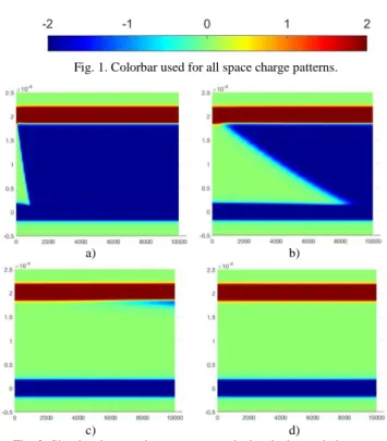
A. Impact of ion mobility
Only A+ is mobile, B- is considered as too big to move. The ion mobility has been changed from 10-14 to 10-17 m2/V/s. It is to note that the color scale for the space charge pattern is the same for all space charge patterns, and is given for charge densities from -2 to 2 C/m3 (Fig. 1). The simulated space charge patterns are given in Fig. 2 for the four mobility values. All the simulations are presented with the influence charges on each electrode, linked to capacitive and to image charges. A Gaussian filter of width 10 µm was introduced to approach patterns usually obtained experimentally. For most of the space charge profiles, even if only the positive ions are mobile, only negative charges are observed. The specific behavior shows that positive ions move towards the ground electrode, leaving a net negative charge next to the top electrode first. This net negative charge, due to immobile negative ions, appears nearer to the ground electrode with time. Positive ions accumulate next to the ground electrode, but are not observed here due to the low quantity of initial ions, and the fact that influence charges at the electrode mask these positive charges. The higher the positive ions mobility, the sooner the material bulk becomes negative. The electric field after 3 hours of voltage application is 3.5 107 V/m at the bottom electrode, i.e. 40% higher than the applied electric field, while the electric field at the top electrode is around 1.5 107 V/m for a positive ion mobility of 10-15 m2/V/s.
Fig. 1. Colorbar used for all space charge patterns.
This variation of the electric field at the electrodes will have a strong impact on the electronic charge generation at the electrodes. The range of mobility values explored is close to the one obtained for electronic charges when we could expect lower mobilities for ions. Increasing the mobility make it possible to observe some specific patterns within 3 hours stressing. Experimentally, such kind of pattern is observed for XLPE (see as example [7]) soon after voltage application. It could mean that i/ the ion mobility is effectively rather high, ii/ the charge that moves after dissociation is not an ion but an electronic charge, iii/ other processes are involved prior to voltage application, and the initial state of charge is not the one that has been taken for these calculations (e.g. mix of electronic and ionic carriers).
Fig. 3 presents the current density as a function of time for the different positive ion mobility values. When ions are present, there is a specific behavior in the current density, i.e. the presence of a ‘plateau’. The higher the ion mobility is the higher the current density on this plateau. When the ion mobility is increased, the drop in the current density appears sooner in time, when most of the mobile ions have crossed the sample and accumulate at the counter electrode. This is also a kind of result observed experimentally in XLPE [8].
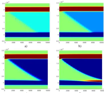
B. Impact of ion concentration
For these simulations, the mobility of positive ions is set to 10-15 m2/V/s, while the negative ions are still immobile. The initial ion concentration has been varied from 0.5 to 10 C/m3. Fig. 4 shows the simulated space charge profiles obtained for different initial ion densities. The space charge pattern does
not change to a large extent when the initial ion density is increased. The dynamic is almost the same for all initial ion densities, the net charge varying slightly. Only when the initial ion density is high (5 C/m3), positive charge accumulation is observed at the counter electrode.
Fig. 3. Simulated current density vs. time for different positive ion mobilities.
As for the previous case, positive charges are present at the vicinity of the cathode, but are masked by the negative charges and the influence charges. When the initial ion density is high, the negative charge density is not enough to mask the presence of positive charges at the cathode. An increase by one decade of the initial ion concentration increases the value of the current density on the plateau by one decade, but does not change the transient current shape (not shown here). Looking at the electric field value at the cathode (Fig. 5), an increase of the initial ion concentration has a large impact on the electric field value. An increase of a decade of the ion density implies a value of electric field which is multiplied by two. This then has a direct impact on the electronic charge injection. Simulations have also been performed for mobile positive and negative ions. The space charge pattern and current density as a function of time for these cases do not change to a large extent as long as negative ions have a lower mobility compared to positive ones. If negative ions have a higher mobility than positive ones, then the charge pattern would be reversed, i.e. a dominant positive charge that seems to arise from the cathode.
a) b)
c) d)
Fig. 2. Simulated space charge patterns calculated when only ions are present, and when only positive ions are mobile, for different mobilities:
Fig. 5. Simulated electric field at the cathode as a function of time for different initial ion concentrations.
IV. COMBINED IONIC AND ELECTRONIC TRANSPORT
For this case study, electronic and ionic species have been considered. The parameters for electronic species are the ones that have been optimized in [2], for a constant effective mobility for electrons and holes, see Table 1. For ionic species the initial ion density is 2 C/m3 and the positive ion mobility is 10-15 m2/V/s. Fig. 6 presents the net charge density as a function of time and space for this case study. A positive charge front is observed arising from the anode. These charges are injected holes that cross the dielectric. The positive charge front disappears slowly in the middle of the sample, progressively replaced by negative charges. These negative charges are the negative ions that cannot move and are ‘uncovered’ progressively by the positive ions leaving their initial position to accumulate at the ground electrode (cathode). These negative ions completely mask the positive charge injection and continuous flow towards the cathode. It is to note that the injection flux does not change to a large extent at the anode, as the net charge density is small. At the cathode however, the positive ion accumulation in this region implies a higher negative charge injection after 3000 s, i.e. when most of the positive ions have migrated towards the cathode. The simulated current density transient associated to this case study is given in Fig. 7. For comparison, the current density when only electronic carriers are considered is also presented. The current density shape is different without and with ions, as a small increase is observed below 10 s, and then the current density is quasi stable during 1000 s.
Fig. 6. Simulated space charge pattern calculated when electronic and ionic carriers are considered, for an initial ion density of 2 C/m3. Applied voltage 5
kV, temperature 25°C.
Fig. 7. Simulated current density function of time calculated for electronic carriers only and when electronic and ionic carriers are considered, for an initial ion density of 2 C/m3. Applied voltage 5 kV, temperature 25°C.
This behavior is directly linked to the movement of positive ions. Once most of them accumulate close to the cathode, the current density decreases, to a value higher than the one calculated without ions. Although ionic and electronic carriers are not considered to interact, the total current is not just the superposition of the two contributions taken independently.
V. CONCLUSIONS
A bipolar charge transport model has been implemented to take into account the presence of positive and negative ions and their transport inside an insulating material. A small amount of ions has a large impact on the space charge density, on the electric field at the electrode, and on the current density. The simulated space charge and current transients has clear common features with what is measured in reality for insulating polymers which are known or supposed to contain ionic contributions to conduction. More work needs now to be done to take into account the neutral molecule impact and the recombination between positive and negative ions as first step.
a) b)
c) d)
Fig. 4. Simulated space charge patterns calculated when only ions are present, and for different ion concentrations:
REFERENCES
[1] G.C. Montanari, "Electrical degradation threshold of polyethylene investigated by space charge and conduction current measurements",
IEEE Trans. Dielectr. Electr. Insul., vol. 7, pp. 309- 315, 2000
[2] S. Le Roy, G. Teyssedre, C. Laurent, G.C. Montanari, and F. Palmieri, "Description of charge transport in polyethylene using a fluid model with a constant mobility: fitting model and experiments", J Phys D:
Appl. Phys., vol. 39, pp. 1427-1436, 2006
[3] K. Kao and W. Hwang, Electrical Transport in Solids, Pergamon Press: New-York, 1981
[4] L.A. Dissado and J.C. Fothergill, Electrical Degradation and
Breakdown in Dielectrics, ed G C Stevens, London: Peter Peregrinus
Ltd, 1992.
[5] S. Le Roy, G. Teyssedre, and C. Laurent, "Modelling space charge in a cable geometry", IEEE Trans. Dielectr. Electr. Insul., vol. 23, pp. 2361−2367, 2016
[6] R. Guffond, "Characterization and modeling of microstructure evolution of cable insulation system under high continuous electric field", PhD Thesis, Sorbonne University, Paris, 2018.
[7] S. Le Roy and G. Teyssedre, "Ion generation and transport in low density polyethylene under electric stress", Proc. IEEE Conf. Electrical
Insulation and Dielectric Phenomena (CEIDP), pp. 63-66, 2015
[8] J. Cènes, G. Teyssedre, S. Le Roy, L. Berquez, P. Hondaâ, V. Eriksson, M. Bailleul, and C. Moreau, "Implementation of space charge measurement using the Pulsed Electro-Acoustic method during ageing of HVDC model cable", Proc. Int. Conf. on Insulated Power Cables, (JiCable-19) Versailles, France, Paper B7-4, pp. 1-6, 2019