Classification decisions in pattern recognition

43

RESEARCH LABORATORY OF ELECTROOICS MASSACHUSETTS INSTITUTE OF TECHNOLOGY CAMBRIDGE 39, MASSACHUSETTS, U.S.A.

CLASSIFICATION DECISIONS IN PATTERN RECOGNITION

QoS

TECHNICAL REPORT 381

APRIL 25, 1960

MASSACHUSETTS INSTITUTE OF TECHNOLOGY

RESEARCH LABORATORY OF ELECTRONICS

CAMBRIDGE, MASSACHUSETTS

The Research Laboratory of Electronics is an interdepartmental laboratory of the Department of Electrical Engineering and the Department of Physics.

The research reported in this document was made possible in part by support extended the Massachusetts Institute of Technology, Research Laboratory of Electronics, jointly by the U. S. Army (Sig-nal Corps), the U.S. Navy (Office of Naval Research), and the U.S. Air Force (Office of Scientific Research, Air Research and Develop-ment Command), under Signal Corps Contract DA36-039-sc-78108, Department of the Army Task 3-99-20-001 and Project 3-99-00-000.

MASSACHUSETTS INSTITUTE OF TECHNOLOGY RESEARCH LABORATORY OF ELECTRONICS

Technical Report 381 April 25, 1960

CLASSIFICATION DECISIONS IN PATTERN RECOGNITION

George S. Sebestyen

This report is based on a thesis, entitled "On Pattern Recognition with Application to Silhouettes," submitted to the Department of Electrical Engineering, M. I. T., August 24, 1959, in partial fulfillment of the require-ments for the degree of Doctor of Science. A portion of the work represents an extension of the thesis and was carried out at Melpar, Inc., Watertown, Massa-chusetts, under Contract AF30(602)-2112.

Abstract

The basic element in the solution of pattern-recognition problems is the requirement for the ability to recognize membership in classes. This report considers the automatic

establishment of decision criteria for measuring membership in classes that are known only from a finite set of samples. Each sample is represented by a point in a suitably chosen, finite-dimensional vector space in which a class corresponds to a domain that contains its samples. Boundaries of the domain in the vector space can be expressed analytically with the aid of transformations that cluster samples of a class and separate classes from one another. From these geometrical notions a generalized discriminant analysis is developed which, as the sample size goes to infinity, leads to decision-making that is consistent with the results of statistical decision theory.

A number of special cases of varying complexity are worked out. These differ from one another partly in the manner in which the operation of clustering samples of a class and the separation of classes is formulated as a mathematical problem, and partly in the complexity of transformations of the vector space which is permitted during the solution of the problem. The assumptions and constraints of the theory are stated, practical considerations and some thoughts on machine learning are discussed, and an illustrative example is given for the automatically learned recognition of spoken words.

TABLE OF CONTENTS

I. Introduction 1

II. A Special Theory of Similarity 5

2. 1 Similarity 5

2. 2 Optimization and Feature Weighting 8

2. 3 Describing the Category 14

2.4 Choosing the Optimum Orthogonal Coordinate System 15

2.5 Summary 19

III. Categorization 21

3. 1 The Process of Classification 21

3. 2 Learning 23

3.3 Threshold Setting 24

3.4 Practical Considerations 26

IV. Categorization by Separation of Classes 32

4. 1 Optimization Criteria 32

4. 2 A Separating Transformation 34

4. 3 Maximization of Correct Classifications 39

V. Nonlinear Methods in Classificatory Analysis 43

5. 1 Enlarging the Class of Transformations 43

5. 2 Geometrical Interpretation of Classification 49

5.3 Some Unsolved Problems 51

VI. General Remarks on Pattern Recognition 54

Acknowledgment 58

Appendix A. The Solution of Eigenvalue Problems 59

Appendix B. Relationship between the Measure of Similarity and the

Likelihood Ratio 63

Appendix C. Automatic Recognition of Spoken Words 67

Appendix D. General Equivalence of the Likelihood Ratio and the

Geometrical Decision Rule 72

Bibliography 75

I

I

I. INTRODUCTION

As the advances of modern science and technology furnish the solutions to problems of increasing complexity, a feeling of confidence is created in the realizability of mathe-matical models or machines that can perform any task for which a specified set of instructions for performing the task can be given. There are, however, problems of long-standing interest that have eluded solution, partly because the problems have not been clearly defined, and partly because no specific instructions could be given on how to reach a solution. Recognition of a spoken word independently of the speaker who utters it, recognition of a speaker regardless of the spoken text, threat evaluation, the problem of making a medical diagnosis, and that of recognizing a person from his handwriting are only a few of the problems that have remained largely unsolved for the above-mentioned reasons.

All of these problems in pattern recognition, however different they may seem, are united by a common bond that permits their solution by identical methods. The common bond is that the solution of these problems requires the ability to recognize membership in classes, and, more important, it requires the automatic establishment of decision criteria for measuring membership in each class.

The purpose of this report is to consider methods of automatically establishing deci-sion criteria for classifying events as members of one or another of the classes when the only knowledge about class membership is from a finite set of their labeled samples.

We shall consider the events represented by points or vectors in an N-dimensional space. Each dimension expresses a property of the event, a type of statement that can be made about it. The entire signal that represents all of the information available about the event is a vector V = (v1, v2 ... vn ... ,vN), the coordinates of which have numerical values that correspond to the amount of each property present in the event. In this repre-sentation, the sequence of events belonging to the same category corresponds to an ensemble of points scattered within some region of the signal space.

The concept playing a central role in the theory that will be described is the notion that the ensemble of points in signal space that represents a set of nonidentical events belonging to a common category must be close to each other, as measured by some - as yet - unknown method of measuring distance, since the points represent events that are close to each other in the sense that they are members of the same category. Mathe-matically speaking, the fundamental notion underlying the theory is that similarity (closeness in the sense of belonging to the same class or category) is expressible by a metric (a method of measuring distance) by which points representing examples of the category we wish to recognize are found to lie close to each other.

To give credence to this idea, consider what we mean by the abstract concept of a class. According to one of the possible definitions, a class is a collection of things that have some common properties. By a modification of this thought, a class could be characterized by the common properties of its members. A metric by which points

2'

T

*-__

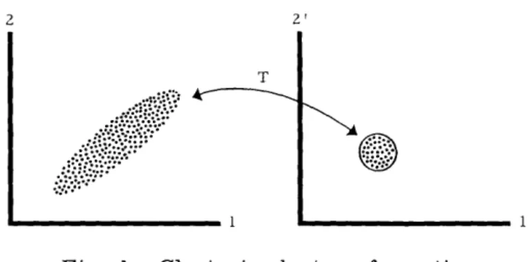
-_I~~~ 1' Fig. 1. Clustering by transformation.

representing samples of a class are close to each other must therefore operate chiefly on the common properties of the samples and must ignore, to a large extent, those prop-erties not present in each sample. As a consequence of this argument, if a metric were found that called samples of the class close, somehow it would have to exhibit their com-mon properties.

In order to present this fundamental idea in a slightly different way, we can state that a transformation on the signal space that is capable of clustering the points representing the examples of the class must operate primarily on the common properties of the

examples. A simple illustration of this idea is shown in Fig. 1, where the ensemble of points is spread out in signal space (only a two-dimensional space is shown for ease in

illustration) but a transformation T of the space is capable of clustering the points of the ensemble. In the example above, neither the signal's property represented by coordi-nate 1 nor that represented by coordicoordi-nate 2 are sufficient to describe the class, for the

spread in each is large over the ensemble of points. Some function of the two coordi-nates, on the other hand, would exhibit the common property that the ratio of the value

of coordinate 2 to that of coordinate 1 of each point in the ensemble is nearly one. In this specific instance, of course, simple correlation between the two coordinates would exhibit this property; but in more general situations simple correlation will not suffice. If the signal space shown in Fig. 1 were flexible (like a rubber sheet), the trans-formation T would express the manner in which various portions of the space must be stretched or compressed in order to bring the points together most closely.

Although thinking of transformations of the space is not as general as thinking about exotic ways of measuring "distance" in the original space, the former is a rigorously correct and easily visualized analogy for many important classes of metrics.

Mathematical techniques will be developed to find automatically the "best" metric or "best" transformation of given classes of metrics according to suitable criteria that establish "best."

As in any mathematical theory, the theory that evolved from the preceding ideas is based on certain assumptions. The first basic assumption is that the N-dimensional sig-nal space representation of events exemplifying their respective classes is sufficiently complete to contain information about the common properties that serve to characterize

2 _ _ ___ _ 2 I

(a·

I

the classes. The significance of this assumption is appreciated if we consider, for example, that the signal space contains all of the information that a black-and-white television picture could present of the physical objects making up the sequence of events which constitute the examples of a class. No matter how ingenious are the data-processing schemes that we might evolve, objects belonging to the category "red things"

could not be identified because representation of the examples by black-and-white tele-vision simply does not contain color information. For any practical situation one must

rely on engineering judgment and intuition to determine whether or not the model of the real world (the signal space) is sufficiently complete. Fortunately, in most cases, this determination can be made with considerable confidence.

A second assumption states the class of transformations or the class of metrics within which we look for the "best." This assumption is equivalent to specifying the allowable methods of stretching or compressing the signal space within which we look for the best specific method of deforming the space. In effect, an assumption of this type

specifies the type of network (such as active linear networks) to which the solution is restricted.

The third major assumption is hidden in the statement that we are able to recognize a "best" solution when we have one. In practice, of course, we frequently can say what is considered a good solution even if we do not know which is the "best." The criterion by which the quality of a metric or transformation is judged good is thus one of the basic assumptions.

Within the constraints of these assumptions, functions of the signal space and the known, labeled sequence of events that permit the separation of events into their respec

-tive categories may be found.

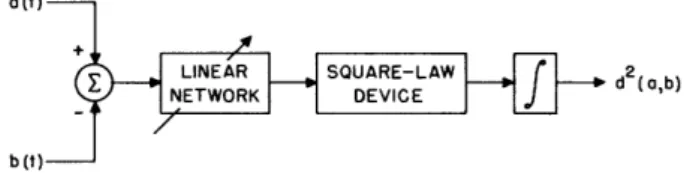
Throughout this report essentially all of the mathematics is developed in simple algebraic form, with only occasional use of matrix notation in places where its use greatly simplifies the symbolism. Insistence on the algebraic form sometimes results in the loss of elegance and simplicity of solutions. But it is felt that the ease of transi-tion from algebra to a computer program is so significant that the loss in the aesthetic appeal of this material to a mathematician must be risked. While the mathematics is thus arithmetized and computer-oriented for practical reasons, we must not lose sight of the broader implications suggested to those who are well versed in communication theory. It is a valuable mental exercise to interpret what is presented here from the point of view of communication theory. To help cross the bridge, at least partially, we can say that passing from the discrete to the continuous, from sum to integral, from dot product to correlation, and from transformation to passage through a linear network (convolution) is valid in all cases in the material contained in this report. The sets of vectors or events are sample functions of a random process, and the metrics obtained are equivalent to different error criteria. The Euclidean metric, for instance, is the mean-square error. The application of other metrics developed in most of this report is equivalent to using the mean-square-error criterion after the signal's passage through

3

a linear network. However, some other metrics developed are error criteria that cannot be equated to a combination of filtering and mean-square-error measurement.

The material presented here is organized in essentially two parts. In Sections II and III a special form of the theory is presented in some detail so that fundamental concepts and the mechanical details of the mathematical developments could be introduced. The highlights of these two sections are the development of the notions of similarity, feature weighting, and the elementary ideas of machine learning. Toward the end of Section III, some practical considerations are pursued, primarily to estimate the storage require-ments of a machine that would implement the numerical calculations.

Discussion of the second part of the material opens in Section IV with the continued application of the linear methods cited in earlier sections to the problem of clustering events that belong to the same category while separating them from those that belong to other categories. Several optimization criteria are considered, and the solutions are derived. The methods of applying the nonlinear methods within the framework of the ideas of this classificatory analysis are discussed in Section V, which also incorporates miscellaneous ideas, some remarks about the limitations of the results, and the direc-tion that might be taken by continuing research. The brief final discussion of some of the important aspects of pattern recognition in Section VI places this work in its proper perspective and relates it to other work in the field. Appendix A discusses a network analog for solving eigenvalue problems rapidly - the most time-consuming mathematical operation encountered in implementing the techniques described. In Appendix B the relationship between decision theory and the theory developed here is explored. Appen-dix C contains a discussion of the numerical application of the special form of the theory to an example in the recognition of spoken words. Appendix D establishes a further con-nection between the theory developed here and the classical problem of statistical hypoth-esis testing.

4

II. A SPECIAL THEORY OF SIMILARITY

2. 1 SIMILARITY

The central problem of pattern recognition is viewed in this work as theproblem of developing a function of a point and a set of points in an N- dimensional space in order to partition the space into a number of regions that correspond to the categories to which the known set of points belongs. A convenient and special but not essential -way of thinking about this partitioning function is to consider it as being formed from a set of functions, one for each category, where each function measures the "likelihood" with which an arbitrary point of the space could best fit into the particular function's own category. In a sense, each function measures the similarity of an arbitrary point of the space to a category, and the partitioning function assigns the arbitrary point to that category to which the point is most similar. (Although the term "likelihood" has an already well-defined meaning in decision theory, it is used here in a qualitative way

x/ _y

(a)

x _y

(b)

Fig. 2. Likelihood of membership in two categories: (a) Category 1; (b) Category 2.

l

R2

(a)

Fig. 3. Classification by maxi-mum likelihood ratio.

(b)

to emphasize the similarity between fundamental ideas in decision theory and in the theory that is described here. )

The foregoing concept of partitioning the signal space is illustrated in Fig. 2, where the signal space has two dimensions and the space is to be partitioned into two cate-gories. In Fig. 2a, the height of the surface above the x-y plane expresses the likeli-hood that a point belongs to Category 1, while that of the surface in Fig. 2b expresses the likelihood that the point belongs to Category 2. The intersection between the two surfaces, shown in Figs. 3a and 3b, marks the boundary between Region 1, where points are more likely to belong to Category 1 than to Category 2, and Region 2, where the reverse is true.

For each category of interest a set of likelihood ratios can be computed that expresses the relative likelihood that a point in question belongs to the category of interest rather than to any of the others. From the maximum of all likelihood ratios that correspond to a given point, we can infer the category to which the point most likely belongs.

The reader will recognize the idea of making decisions based on the maximum

likelihood ratio as one of the important concepts of decision theory. The objective of the preceding discourse is, therefore, simply to make the statement that once afunction measuring the likelihood that a point belongs to a given category is developed, there is

at least one well- established precedent for partitioning signal space into regions that are associated with the different categories. The resulting regions are like a template that serves to classify points on the basis of their being covered or not covered by the template. Although in the rest of this section, partitioning the signal space is based on a measure of similarity that resembles the likelihood ratio only in the manner in which it is used, it is shown in Appendix B that, in certain cases, decisions based on the measure of similarity are identical with those based on the maximum likelihood ratio.

In the first three sections of this report, a quantitative measure of similarity is developed in a special theory in which similarity is considered as a property of only the point to be compared and the set of points that belongs to the category to be learned. In later sections we shall discuss methods for letting known nonmembers of the class influence the development of measures of similarity.

In the special theory, similarity of an event P to a category is measured by the closeness of P to every one of those events {Fm) known to be contained in the category. Similarity S is regarded as the average "distance" between P and the class of events represented by the set {Fm} of its examples. Two things should be noted about this foregoing definition of similarity. One is that the method of measuring distance does not influence the definition. Indeed, "distance" is not understood here in the ordinary Euclidean sense; it may mean "closeness" in some arbitrary, abstract property of the set {Fm} that has yet to be determined. The second thing to note is that the concept of distance between points, or distance in general, is not fundamental to a concept of

similarity. The only aspect of similarity really considered essential is that it is a real valued function of a point and a set that allows the ordering of points according to their

similarity to the set. The concept of distance is introduced as a mathematical venience based on intuitive notions of similarity. It will be apparent later how this con-cept forms part of the assumptions stated in Section I as underlying the theory to be presented. Even with the introduction of the concept of distance there are other ways of defining similarity. Nearness to the closest member of the set is one possibility. This implies that an event is similar to a class of events if it is close in some sense to any member of the class. We shall not philosophize on the relative merits of these

differ-ent ways of defining similarity. Their advantages and disadvantages will become apparent as this theory is developed, and the reader will be able to judge for himself which set of assumptions is most applicable under a given set of circumstances. The essential role of the definition of similarity and the choice of the class of metrics within which the optimum is sought is to define the decision rule with which membership in

classes will be determined. The decision rule, of course, is not an a priori fixed rule; it contains an unknown function, the unspecified metric, which will be tailored to the particular problem to be solved. For the time being, the decision rule will remaini an

ad hoc rule; it will be shown later that it is indeed a sound rule.

To summarize the foregoing remarks, for the purpose of the special theory, simi-larity S(P, Fm}) of a point P and a set of points {Fm} exemplifying a class will be defined as the mean- square distance between the point P and the M members of the set {Fm}. This definition is expressed by Eq. 1, where the metric d( ) - the method of measuring distance between two points - is left unspecified.

M

S(PJFm}) M d(PFm) (1)

To deserve the name metric, the function d( ) must satisfythe usual conditions stated in Eqs. 2.

d(A,B) = d(B,A) (symmetric function) (2a)

d(A,C) - d(A,B) + d(B,C) (triangle inequality) (2b)

d(A,B) > 0 (non-negative) (2c)

d(A,B) = 0 if, and only if, A = B (2d)

2.2 OPTIMIZATION AND FEATURE WEIGHTING

In the definition of similarity of Section 2.1, the mean- square distance between a point and a set of points served to measure similarity of a point to a set. The method of measuring distance, however, was left unspecified and was understood to refer to distance in perhaps some abstract property of the set. Let us now discuss the criteria for finding the "best" choice of the metric, and then applythis optimizationto a specific and simple class of metrics that has interesting and useful properties.

Useful notions of "best" in mathematics are often associated with finding the extrema of the functional to be optimized. We may seek to minimize the average cost of our decisions or we may maximize the probability of estimating correctly the value of a random variable. In the problem above, a useful metric, optimal in one sense, is one that minimizes the mean- square distance between members of the same set, subject to certain suitable constraints devised to ensure a nontrivial solution. If the metric is thought of as extracting that property of the set in which like events are clustered, the mean- square distance between members of the set is a measure of the size of the cluster so formed. Minimization of the mean- square distance is then a choice of a metric that minimizes the size of the cluster and therefore extracts that property of the set in which they are most alike. It is only proper that a distance measure shall minimize distances between those events that are selected to exemplify things that are "close."

Although the preceding criterion for finding the best solution is a very reasonable and meaningful assumption on which to base the special theory, it is by no means the only possibility. Minimization of the maximum distance between members of a set is just one of the possible alternatives that immediately suggests itself. It' should be

pointed out that ultimately the best solution is the one which results in the largest number of correct classifications of events. Making the largest number of correct decisions on the known events is thus to be maximized and is itself a suitable criterion of optimization that will be dealt with elsewhere in this report. Since the primary purpose of this section is to outline a point of view regarding pattern recognitionthrough a special example, the choice of "best" previously described and stated in Eq. 3 will be used, for it leads to very useful solutions with relative simplicity of the mathematics involved. In Eq. 3, Fp and Fm are the pth and mth members of the set {Fm}

mi 2 p,m F m1

minLd

(FPm)

IV

(M-l)

=

1

=

(3) Of the many different mathematical forms that a metric may take, in our special theory only metrics of the form given by Eq. 4 will be considered. The intuitive notions underlying the choice of the metric in this form are based on ideas of "feature weighting," which will be developed below.

d(A,B) = Ln W (an-bn) (4)

In the familiar Euclidean N-dimensional space the distance between the two points A and B is defined by Eq. 5. If A and B are expressed in terms of an orthonormal coordinate system {n}, then d(A,B) of Eq. 5 can be written as in Eq. 6, where an and bn, respectively, are the coordinates of A and B in the direction of n.

d(A,B) =I A-B 1 (5)

FN 1 1/2

d(A, B) = (an bn) (6)

We must realize, of course, that the features of the events represented bythe differ-ent coordinate directions n are not all equally important in influencing the definition of the category to which like events belong. Therefore it is reasonable that in comparing two points feature by feature (as expressed in Eq. 6), features with decreasing signifi-cance should be weighted with decreasing weights, Wn. The idea of feature weighting is expressed by a metric somewhat more general than the conventional Euclidean metric. The modification is given in Eq. 7, where Wn is the feature weighting coefficient.

d(A,B) = [Wn(an- bn) ] (7)

n=1W ,

It is readily verified that the above metric satisfies the conditions stated in Eq. 2 if none of the Wn coefficients is zero; if any of the Wn coefficients is zero, Eq. 2d is not satisfied.

9

It is important to note that the metric above gives a numerical measure of "close-ness" between two points, A and B, that is strongly influenced by the particular set of

similar events {Fm}. This is a logical result, for a measure of similarity between A and B should depend on how our notions of similarity were shaped by the set of events known to be similar. When we deal with a different set of events that have different similar features, our judgment of similarity between A and B will also be based on finding agreement between them among a changed set of their features.

An alternative and instructive way of explaining the significance of the class of met-rics given in Eq. 4 is to recall the analogy made in Section I regarding transformations of the signal space. There, the problem of expressing what was similar among a set of events of the same category was accomplished by finding the transformation of the signal space (again, subject to suitable constraints) that will most cluster the transformed events in the new space. If we restrict ourselves to those linear transformations of the signal space that involve only scale factor changes of the coordinates and if we measure distance in the new space by the Euclidean metric, thenthe Euclidean distance between two points after their linear transformation is equivalent to the feature weighting metric of Eq. 4. This equivalence is shown below, where A' and B' are vectors obtained from A and B by a linear transformation. The most general linear transfor-mation is expressed by Eq. 9, where a' _n is the nth coordinate of the transformed vector A, and b' _n is that of the vector B.

N N

A

Z

nn n

n=1 n1 n

[A'] = [A] [W] [B'] = [B] [W] (8b)

[A'-B'] = [A-B][W] (8c)

[(a'-b') (a'-b), _{1 1,2 2 (a .}(a' -b' )]_b

N )]

= [(al-bl), (a2 -b2) .. , (aN-bN)]

W1 1 w1 2 .·. WlN

w2 1 w2 2 . . w 2N

WN1 WN2 ' ' ' WNN The Euclidean distance between A' and B', dE(A', B'), is given in Eq. 10.

dE(A',B') - (an s b

}

If the linear transformation involves only scale factor changes of the coordinates, only the elements on the main diagonal of the W matrix are nonzero, and thus dE(A', B')

is reduced, in this special case, to the form given in Eq. 11.

10

Special dE(A'. B') = w n(an n) (11)

The preceding class of metrics will be used in Eq. 3 to minimize the mean-square distance between the set of points.

The mathematical formulation of the minimization is given in Eqs. lZa and 12b. The significance of the constraint of Eq. 12b is, for the case considered, that every weight wnn is a number between 0 and 1 (the wnn turn out to be positive) and that it can be interpreted as the fractional value of the features On that they weight. The fractional value that is assigned in the total measure of distance to the degree of agreement that exists between the components of the compared vectors is denoted by wnn'

2 1 M M N 2 2 minimize D pl 1 1 W(fmnmfpn) (12a) M(M-1) = =1 n_ if N E wnn =1 (12b) nn

Although the constraint of Eq. 12b is appealing from a feature-weighting point of view, from a strictly mathematical standpoint it leaves much to be desired. It does not guarantee, for instance, that a simple shrinkage in the size of the signal space is disallowed. Such a shrinkage would not change the relative orientation of the points to each other, the property really requiring alteration. The constraint given in Eq. 13, on the other hand, states that the volume of the space is constant, as if the space were filled with an incompressible fluid. Here one merely wishes to determine the kind of rectangular box that could contain the space so as to minimize the mean- square distance among a set of points imbedded in the space.

N

w nn=1 (13)

n=1

The minimization problem with both of these constraints will be worked out in the following equations; the results are quite similar.

Interchanging the order of summations and expanding the squared expression in Eq. 12a yield Eq. 14, where it is recognized that the factor multiplying wnn is the variance of the coefficients of the n coordinate. Minimization of Eq. 14 under the constraint of Eq. 12b yields Eq. 15, where p is an arbitrary constant. Imposing the constraint of Eq. 12b again, we can solve for wnn, obtaining Eq. 16.

2 M +

D = wnn I M f -2 m fPj f (14a)

(M-l)n 1 m

n

11

2 2M w2 2M N 2 2 (M-1) n=l (M-1) n=1 L-wnn'rnP ]=o n = 1, 2, ... , N (15) P 1 Wnn 2 N (16) a- 2 1 n an Z 2 p=l P

(Note that this result is identical with that obtained in determining the coefficients of combination in multipath combining techniques encountered in long-distance communi-cations systems.)

That the values of wnn so found are indeed those that minimize D2 of Eq. 12a can be seen by noting that D2 is an elliptic paraboloid in an N-dimensional space and the constraint of Eq. 12b is a plane of the same dimensions. For a three-dimensional case, this is illustrated in Fig. 4. The intersection of the elliptic paraboloid with the plane is a curve whose only point of zero derivative is a minimum.

D2

ANE

Fig. 4. Geometric interpretation

MINIMUM of minimization.

If the variance of a coordinate of the ensemble is large, the corresponding wnn is small, which indicates that small weight is to be given in the over- all measure of distance to a feature of large variation. But if the variance of the magnitude of a given coordi-nate 0n is small, its value can be accurately anticipated. Therefore 0n should be

counted heavily in a measure of similarity. It is important to note that in the extreme case, where the variance of the magnitude of a component of the set is zero, the

corre-sponding wnn in Eq. 16 is equal to one, with all other wnn equal to zero. In this case, although Eq. 11 is not a legitimate metric, since it does not satisfy Eq. 2, it is still a meaningful measure of similarity. If any coordinate occurs with identical magnitudes in all members of the set, then it is an "all-important" feature of the set, and nothing

12

else needs to be considered in judging the events similar. Judging membership in a category by such an "all-important" feature may, of course, result in the incorrect inclusion of nonmembers in the category. For instance "red, nearly circular figures" have the color red as a common attribute. The transformation described thus far would pick out "red" as an all-important feature and would judge membership in the category of "red, nearly circular figures" only by the color of the compared object. A red

square, for instance, would thus be misclassifiedand judged tobe a "red, nearly circu-lar figure." Given only examples of the category, such results would probably be expected. In Section IV, however, wherelabeled examples of all categories of interest are assumed given, only those attributes are emphasized in which members of a cate-gory are alike and in which they differ from the attributes of other categories.

Note that the weighting coefficients do not necessarily decrease monotonically in the feature weighting, which minimizes the mean- square distance among M given examples of the class. Furthermore, the results of Eqs. 16 or 18 are independent of the particu-lar orthonormal system of coordinates. Equations 16 and 18 simply state that the weighting coefficient is inversely proportional to the variance or to the standard devi-ation of the ensemble along the corresponding coordinate. The numerical values of the variances, on the other hand, do depend on the coordinate system.

If we use the mathematically more appealing constraint of Eq. 13 in place of that in Eq. 12b, we obtain Eq. 17.

N 2 2 N

min D = min 2 w 1 (17a)

n1 nn n nn

N 2 N

Zn dw nnn - X w =0 (1 7b)

n=1 w k~n

It is readily seen that by applying Eq. 17a, the expression of Eq. 17b is equivalent to Eq. 18a, where the bracketed expression must be zero for all values of n. This substitution leads to Eq. 18b, which may be reduced to Eq. 18c by applying Eq. 17a once more.

N

1

Thus it is seen that the feature weighting coefficient w is proportional to the th and thereby lends itself to the reciprocal standard deviation of the n coordinates, and thereby lends itself to the same interpretation as before.

13

2.3 DESCRIBING THE CATEGORY

The set of known members is the best description of the category. Following the practice of probability theory, we can describe this set of similar events by its statistics; the ensemble mean, variance and higher moments can be specified as its characteristic properties. For our purpose a more suitable description of our idea of the category is found in the specific form of the function S of Eq. 1 developedfrom the set of similar events to measure membership in the category. A marked disadvantage of S is that (in a machine that implements its application) the amount of storage capacity that must be available is proportional to the number of events introduced and is thus a growing quantity. Note that S(P,{Fm}) can be simplified and expressed in terms of certain statistics of the events,which makes it possible to place an upper bound on the storage requirements demanded of a machine.

Interchanging the order of summations and expanding the squares yield Eq. 19a, 2

which, through the addition and subtraction of fn , yields Eq. 19b.

S({} M N 2 f 2 N 2 2 (19a)

mS(P'(fFm) M _{m=1 n1}

-1

N 2+ 22 N 2

= X WnlP-f) + W(Pn-fn) (19b)

n1 1

We see that the category can be described by first- and second-order statistics of the given samples. This fact also reveals the limitations of the particular class of metrics considered above, for there are classes for which first- and second-order statistics are not sufficient descriptors. It should be pointed out, however, that this is a limi-tation of the particular, restricted class of metrics just considered, rather than a limitation of the approach used.

By substituting Wn from Eq. 18 in the quadratic form of Eq. 19, we obtain

/N N Pn- N

S(P,{F ) = X n + ]

1

Contours of constant S(P,{Fm}) are ellipses centered at f, where f is the sample mean, and the diameters of the ellipse are the variances of the samples in the directions of the coordinate axes.

The set of known members of the category appears as the constants fn and n- , which may be computed once and for all. Since these constants can be updated readily without recourse to the original sample points, the total number of quantities that must be stored is fixed at 2N and is independent of the number of sample points.

2.4 CHOOSING THE OPTIMUM ORTHOGONAL COORDINATE SYSTEM

The labeled events that belong to one category have been assumed given as vectors in an assumed coordinate system that expressed features of the events thought to be relevant to the determination of the category. An optimum set of feature weighting coefficients through which similar events could be judged most similar to one another was then found. It would be purely coincidental, however, if the features represented by the given coordinate system were optimal in expressing the similarities among members of the set. In this section, therefore, we look for a new set of coordinates, spanning the same space and expressing a different set of features that minimize the mean-square distance between members of the set. The problem just stated can be thought of as either enlarging the class of metrics considered thus far in the measure of similarity defined earlier or as enlarging the class of transformations of the space within which class we look for that particular transformation that minimizes the

mean-square distance between similar events.

It was proved earlier that the linear transformation that changes the scale of the nt h dimension of the space by the factor wnn while keeping the volume of the space constant and minimizing the mean- square distance between the transformed vectors is given by

Eq. 22. 0 w 2 F' = F[W] [W] = (22a) WNN and N 1/N W = 1 (22b) p=l n

The mean- square distance under this transformation is a minimum for the given choice of orthogonal coordinate system. It is given by

M M N

2 1 2 2

D = 1 p n w nn(fmn- fpn) = minimum (23)

M(M-1) p=1 m1 n=1

It is possible, however, to rotate the coordinate system until one is found that minimizes this minimum mean-square distance. While the first minimization took place with respect to all choices of the wnn coefficients, we are now interested in further mini-mizing D2 by first rotating the coordinate system so that the above optimum choice of the wnn should result in the absolute minimum distance between vectors. The solution of this search for the optimum transformation can be conveniently stated in the form of the following theorem.

15

THEOREM

The orthogonal transformation which, after transformation, minimizes the mean-square distance between a set of vectors, subject to the constraint that the volume of the space is invariant under transformation, is a rotation [C] followed by a diagonal trans-formation [W]. The rows of the matrix [C] are eigenvectors of the covariance matrix

[U] of the set of vectors, and the elements of [W] are those given in Eq. 22b, where -is the standard deviation of the coefficients of the set of vectors in the direction of the pth eigenvector of [U].

PROOF

Expanding the square of Eq. 23 and substituting the values of wnn result in Eq. 24, which is to be minimized over all choices of the coordinate system.

N M M 2 2 D = w nn

X

~

Let the given coordinate system be transformed by the matrix [C]:

cll C1 2 ... C1N c2 1 c2 2 ... C2N CNi CN2 ... CNN N 2 where Cpn =1 =l, 2,..., N (25) n=l

Equation 24 is minimized if the bracketed expression in Eq. 24c, which we shall name

p, is minimized. N N M M 2 P PM m ( m ) -M fmp (26a) pl P p1l m=l =1 where N fp= nX fmnc (26b) mp = 1 m pn

Substituting Eq. 26b into Eq. 26a, we obtain

N N

_i=

in which the averaging is understood to be over the set of M vectors. The squared expression may be written as a double sum and the entire equation simplified to

N p= l p=l N N n - ff c pncs n= 1 n s

)

But (fnfs-fnfs) = uns = usn is an element of the covariance matrix [U]. Hence we have

ns n n N P= TT p=l N N

Z

Using the method of Lagrange multipliers to minimize in Eq. 29, subject to the constraint of Eq. 25, we obtain Eq. 30 as the total differential of . The differential of the constraint, y, is given in Eq. 31.

dp(C1 1C 1 2 ... CNN) N N a n-1

s=1

pn p

ac

a-1

By way of an explanation of Eq. 30, note that when Eq. 29 is differentiated with respect to c q, then all of the factors in the product in Eq. 29, where p * 1, are simply constants. Carrying out the differentiation stated in Eq. 30, we obtain

N N dp =2

Z

and note that since p * , A is just a constant as regards optimization of any Clx. In accordance with the method of Lagrange multipliers, each of the N constraints of Eq. 31 is multiplied by a different arbitrary constant B and is added to d3 as shown below. N N dp+

Z

Z

b

Lif

By letting - I = B1/A i and by recognizing that dcl q is arbitrary, we get

17 N 1=1 N N q=1 p+ (30) (31) (32) _ ·_ __

N

b=l C bUqb - Xq = 0

b=l P 'P q

q=l, 2,..., N; 1=1, 2,..., N

Let the th row of the [C] matrix be the vector C. Then Eq. 35 can be written as the eigenvalue problem of Eq. 36 by recalling that uqb = Ubq

C[U-XI] = (36)

Solutions of Eq. 36 exist only for N specific values of Xk. The vector C1 is an eigenvector of the covariance matrix [U]. The eigenvalues AX are positive, and the corresponding eigenvectors are orthogonal, since the matrix [U] is positive definite. Since the transformation [C] is to be nonsingular, the different rows C1 must corre-spond to different eigenvalues of [U] . It may be shown that the only extremum of is a minimum, subject to the constraint of Eq. 25. Thus the optimum linear transformation that minimizes the mean- square distance of a set of vectors while keeping the volume of the space constant is given by Eq. 37, where rows of [C] are eigenvectors of the co-variance matrix [U] .

alN a2N a11 a12

a21a22

aN1 aN2 aNN

. . .N . . .2N c1 1c12 c21c22 CNiCN2 CNN T lw22 WNNCN1 WNNCN2 WllCll2 Wllc2 WllClN w2 2c2N WNNCNN WNN (37)

The numerical value of the minimum mean- square distance may now be computed as follows. The quantity D2 was given in Eq. 24c, which is reproduced here as Eq. 38:

D2 - M 2N (M-l) N 21/N P TT(r - M 2N() 1/N (M-l)

Substituting from Eq. 29, we obtain

2 _{M 2N} (M-l) N

p=l

But from Eq. 35 we see that min D2 may be written as

18 (35) (38) (39) w22c21 w22c22 I

min D2 - M 2N N = M 2NT 1 (40)

(M-1) =1 nl (M-1) p=l

in which the constraint of Eq. 25 has been used.

It should be noted that the constraint of Eq. 25 is not, in general, a constantvolume constraint. Instead, the constraint holds the product of the squared lengths of the sides of all N-dimensional parallelepipeds a constant. If, as in the solution just obtained, the

transformation [C] is orthogonal, the volume is maintained constant. A subset of the constant volume transformations, Tv (Fig. 5), are the orthogonal transformations T of constant volume of which the optimum was desired. The solution pre-sented here found the optimum transformation among a set of TL that contains orthogonal transformations of constant volume

har i nt u fc-.;::+rvra+r n rr,,rvl+m fr-r +1-,har h+ r-

nr,-Fig. 5. Sets of trans- orthogonal. The solution given here, therefore, is optimum formations. among the constant volume transformations TnTL shown as

the shaded area in Fig. 5. This intersection is a larger set of transformations than that for which the optimum was sought. The methods of this section are optimal in measuring membership in categories of certain types. Suppose, for instance, that categories are random processes that gener-ate members with multivarigener-ate Gaussian probability distributions of unknown means and variances. In Appendix B we show that the metric developed here measures contours of equal a posteriori probabilities. Given the set of labeled events, the metric speci-fies the locus of points that are members of the category in question with equal probability.

2.5 SUMMARY

Categorization, the basic problem of pattern recognition, is regarded as the process of learning how to partition the signal space into regions where each contains points of only one category. The notion of similarity between a point and a set of points of a category plays a dominant role in the partitioning of signal space. Similarity of a point to a set of points is regarded as the average "distance" between the point and the set. The sense in which distance is understood is not specified, but the optimum sense is thought to be that which (by the optimum method of measuring distance) clusters most

highly those points that belong to the same category. The mean- square distance between points of a category is a measure of clustering. An equivalent alternate interpretation

of similarity (not as general as the interpretation above) is that the transformation that optimally clusters like points, subject to suitable criteria to ensure the nontriviality of the transformations, is instrumental in exhibiting the similarities between points of a

set. In particular, the optimum orthogonal transformation, and hence a non-Euclidean method of measuring distance, is found that minimizes the mean-square distance

between a set of points, if the volume of the space is held constant to ensure nontrivi-ality. The resulting measure of similarity between a point P and a set (Fm} is

S(P,{F ) = M1 ns(Ps E a ms) (41)

where a _ns is given in the theorem of section 2.4.

Classification of an arbitrary point P into one of two categories, F or G, is accomplished by the decision rule given in Eq. 42, where the functions Sf and Sg are obtained from samples of F and samples of G, respectively.

decide P E F if Sf(P,(Fm}) < Sg(P,{Gm})

decide P E G if Sf(P,(Fm_m ) > S g(P,{G _{g m})) (42)

20

III. CATEGORIZATION

3. 1 THE PROCESS OF CLASSIFICATION

Pattern recognition consists of the twofold task of "learning" what the category or class is to which a set of events belongs and of deciding whether or not a new event belongs to the category. In this section, details of the method of accomplishing these two parts of the task are discussed, subject to the limitations on recognizable categories

imposed by the assumptions stated earlier. These details are limited to the application of the special method of Section II.

In the following section two distinct modes of operation of the recognition system will be distinguished. The first consists of the sequential introduction of a set of events, each

labeled according to the category to which it belongs. During this period, we want to identify the common pattern of the inputs that allows their classification into their

respective categories. As part of the process of learning to categorize, the estimate of what the category is must also be updated to include each new event as it is introduced. The process of updating the estimate of the common pattern consists of recomputing the new measures of similarity so that they will include the new, labeled event on which the

quantitative measures of similarity are based.

During the second mode of operation the event P, which is to be classified, is com-pared to each of the sets of labeled events by the measure of similarity found best for each set. The event is then classified as a member of that category to which it is most similar.

It is not possible to state with certainty that the pattern has been successfully learned or recognized from a set of its samples because information is not available on how samples were selected to represent the class. Nevertheless, it is possible to obtain a quantitative indication of our certainty of having obtained a correct method of deter-mining membership in the category from the ensemble of similar events. As each new event is introduced, its similarity to the members of the sets already presented is meas-ured by the function S defined in Section II. The magnitude of the number S indicates how close the new event is to those already introduced. As S is refined and, with each new example, improves its ability to recognize the class, the numerical measure of similarity between new examples and the class will tend to decrease, on the average. Strictly speaking, of course, this last statement cannot be true, in general. It may be true only if the categories to be distinguished are separable by functions S taken from the class that we have considered; even under this condition the statement is true only if certain assumptions are made regarding the statistical distribution of the samples on which we learn. In cases in which no knowledge regarding the satisfaction of either of these two requirements exists, the convergence of the similarity as the sample size is

It is true for Gaussian processes.

21

L L - - - --- j

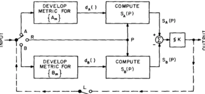
Fig. 6. Elementary block diagram of the classification process.

increased is simply wishful thinking the heuristic justification of which is based on the minimization problem solved in developing S.

Figure 6 illustrates the mechanization of the learning and recognition modes of the special classificatory process discussed thus far. For the sake of clarity, the elemen-tary block diagram of the process distinguishes only between two categories of events, but it can be readily extended to distinguish between an arbitrary number of categories. It should be noted that one of the categories may be the complement of all others. The admission of such a category into the set is only one of the ways in which a machine that is always forced to classify events into known categories may be made to decide that an event does not belong to any of the desired ones; it belongs to the category of "every-thing else." Samples of "every"every-thing else" must, of course, be given.

During the first mode of operation, the input to the machine is a set of labeled events. Let us follow its behavior through an example. Suppose that a number of events, some belonging to set A and some to set B, have already been introduced. According to the method described in Section II, therefore, the optimum metrics (one for each class) that minimize the mean-square distance between events of the same set have been found. As a new labeled event is introduced (say that it belongs to set A), the switch at the input is first turned to the recognition mode R so that the new event P can be compared to set A as well as to set B through the functions SA(P) = S(P, {Am}) and SB(P), which were computed before the introduction of P. The comparison of SA and SB with a threshold K indicates whether the point P would be classified as belonging to A or to B from knowl-edge available up to the present. Since the true membership of P is known (the event is labeled), we can now determine whether P would be classified correctly or incorrectly.

The input switch is then turned to A so that P, which indeed belongs to A, can be included in the computation of the best metric of set A.

When the next labeled event is introduced (let us say that it belongs to set B), the input switch is again turned to R in order to test the ability of the machine to classify the new event correctly. After the test, the switch is turned to B so that the event can be included among examples of set B and the optimum function SB can be recomputed.

This procedure is repeated for each new event, and a record is kept of the rate at which incorrect classifications would be made on the known events. When the training period

22

I- a-Z

is completed, presumably as a result of satisfactory performance on the selection of known events (sufficiently low error rate), the input switch is left in the recognition mode.

3. 2 LEARNING

"Supervised learning" takes place in the interval of time in which examples of the categories generate ensembles of points from which the defining features of the classes are obtained by methods previously discussed. "Supervision" is provided by an outside source such as a human being who elects to teach the recognition of patterns by examples and who selects the examples on which to learn.

"Unsupervised learning," by contrast, is a method of learning without the aid of such an outside source. It is clear, at least intuitively, that the unsupervised learning of membership in specific classes cannot succeed unless it is preceded by a period of super-vision during which some concepts regarding the characteristics of classes are

estab-lished. A specified degree of certainty concerning the patterns has been achieved in the form of a sufficiently low rate of misclassification during the supervised learning period. The achievement of the low misclassification rate, in fact, can be used to signify the end of the learning period, after which the system that performs the operations indicated in Fig. 6 can be left to its own devices. It is only after this supervised interval of time that the system can be usefully employed to recognize, without outside aid, events as belonging to one or another of the categories.

Throughout the period of learning on examples, each example is included in its proper set of similar events that influence the changes of the measures of similarity. After supervised activity has ceased, events introduced for classification may belong to any of the categories; and no outside source informs the machine of the correct category. The machine itself, operating on each new event, however, can determine, with the already qualitatively specified probability of error, to which class the event should belong. If the new event is included in the set exemplifying this class, the function measuring membership in the category has been altered. Unsupervised learning results from the successive alterations of the metrics, brought about by the inclusion of events into the sets of labeled events according to determinations of class membership rendered by the machine itself. This learning process is instrumented by the dotted line in Fig. 6, which, when the learning switch L is closed, allows the machine's decisions to control routing of the input to the various sets.

To facilitate the illustration of some implications of the process described above, consider the case in which recognition of membership in a single class is desired and all labeled events are members of only that class. In this case, classification of events as members or nonmembers of the category degenerates into the comparison of the similarity S with a threshold T. If S is greater than T, the event is a nonmember; if S is less than T, the event is said to be a member of the class. Since the machine decides that all points of the signal space for which S is less than T are members of

P3 \ 'ArA

-; -2

D₁

Fig. 7. Unsupervised learning.

the class, the class - as far as the machine is concerned - is the collection of points that lie in a given region in the signal space. For the specific function S of Section II, this region is an ellipsoid in the N-dimensional space.

Unsupervised learning is illustrated graphically in Fig. 7. The two-dimensional ellipse drawn with a solid line signifies the domain D1 of the signal space in which any

point yields S < T. This domain was obtained during supervised activity. If a point P is introduced after supervised learning, so that P1 lies outside D1, then P1 is merely

rejected as a nonmember of the class. If point P2 contained in D1 is introduced,

how-ever, it is judged a member of the class and is included in the set of examples used to generate a new function S and a new domain D2, designated by the dotted line in Fig. 7.

A third point P₃' which was a nonmember before the introduction of P2, becomes recog-nized as a member of the class after the inclusion of P2 in the set of similar events.

Although the tendency of this process of "learning" is to perpetuate the original domain, it has interesting properties worth investigating. The investigation of unsuper-vised learning would form the basis for a valuable continuation of the work presented herein.

Before leaving the subject of unsupervised learning, we point out that as the new domain D₂ is formed, points such as P4 in Fig. 7 become excluded from the class. Such

an exclusion from the class is analogous to "forgetting" because of lack of repetition. Forgetting is the characteristic of not recognizing P4 as a member of the class, although

at one time it was recognized as belonging to it. 3. 3 THRESHOLD SETTING

In the classification of an event P, the mean-square distance between P and members of each of the categories is computed. The distance between P and members of a cate-gory C is what we called "similarity", Sc(P), in which the "sense" in which "distance" is understood depends on the particular category in question. We then stated that, in a manner analogous to decisions based on maximum likelihood ratios, the point P is clas-sified as a member of the category to which it is most similar. Hence, P belongs to category C if Sc(P) is less than Sx(P), where X is any of the other categories.

Since in this special theory the function SC(P), which measures membership in cate-gory C, was developed by maximally clustering points of C without separating them from points of other sets, there is no guarantee, in general, that a point of another set B may

Se4

S83

S8 2

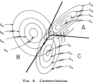
Fig. 8. Categorization.

not be closer to C than to B. This is guaranteed only if points of the sets occupy dis-jointed regions. A graphical illustration that clarifies the comparison of similarities of a point to the different categories is shown in Fig. 8. In this figure the elliptical con-tours SA (P), SA (P), .... indicate the locus of points P in the signal space that is at

1 2

a mean-square distance of 1, 2, . , from members of category A. The loci of these points are concentric ellipsoids in the N-dimensional signal space, shown here in only two dimensions. Similarly, SB (P), SB (P), ... , and S_C (P), SC (P) ... are the loci of those points whose mean-square distance from categories B and C, respectively, are 1, 2 .... Note carefully that the sense in which distance is measured at each of the categories differs as is indicated by the different orientations and eccentricities of the ellipses. The heavy line shows the locus of points that are at equal mean-square distances from two or more sets according to the manner in which distance is measured to each set. This line, therefore, defines the boundary of each of the categories.

At this point in the discussion it will be helpful to digress from the subject of thresh-olds and dispel some misconceptions that Fig. 8 might create regarding the general nature of the categories found by the method that we described. Recall that one of the possible ways in which a point not belonging to either category could be so classified was by establishing a separate category for "everything else" and assigning the point to the category to which its mean-square distance is smallest. Another, perhaps more practical, method is to call a point a member of neither category if its mean-square distance to the set of points of any class exceeds some threshold value. If this threshold value is set, for example, at a mean-square distance of 3 for all of the categories in Fig. 8, then points belonging to A, B, and C will lie inside the three ellipses shown in Fig. 9.

25

It is readily seen, of course, that there is no particular reason why one given mini-mum mean-square distance should be selected instead of another; or, for that

r- -r 4h4- t i1i- 4 A4 -_ - -h A

IlliLLtU , WILy Llllb /III.Ll±±ilUi 1 ULLidIllA;C 0IIUUlU

be the same for all categories. Many logi-cal and useful criteria may be selected for determining the optimum threshold setting. Here, only one criterion will be singled out as particularly useful. This criterion

... . t-- -- A--'---' . . ... .-1. _ _ requires mat me minimum nresnolas De Fig. 9. Categorization with threshold. set so that most of the labeled points fall

into the correct category. This is a funda-mental criterion, for it requires the system to work best by making the largest number of correct decisions. In decision theory the threshold value depends on the a priori probabilities of the categories and on the costs of false alarm and false dismissal.

The criterion of selecting a threshold that will make the most correct classifications can be applied to our earlier discussions in which the boundary between categories was determined by equating the similarities of a point to two or more categories. In the par-ticular example of Fig. 6, where a point could be a member of only one of two categories A and B, the difference SA - SB = 0 formed the dividing line. There is nothing magical about the threshold zero; we might require that the dividing line between the two cate-gories be SA - SB = K, where K is a constant chosen from other considerations. A similar problem in communication theory is the choice of a signal-to-noise ratio that serves as the dividing line between calling the received waveform "signal" or calling it

"noise. " It is understood, of course, that signal-to-noise ratio is an appropriate crite-rion on which to base decisions (at least in some cases), but the particular value of the ratio to be used as a threshold level must be determined from additional requirements. In communication theory these are usually requirements on the alarm or false-dismissal rates. In the problem of choosing the constant K, we may require that it be selected so that most of the labeled points lie in the correct category.

3.4 PRACTICAL CONSIDERATIONS

In considering the instrumentation of the process of categorization previously described, two main objectives of the machine design must receive careful consideration.

The first is the practical requirement that all computations involved in either the learning or the recognition mode of the machine's operation shall be performed as rapidly as possible. It is especially desirable that the classification or recognition of a new event be implemented in essentially real time. The importance of this requirement is readily appreciated if the classificatory technique is considered in terms of an application such

26