HAL Id: hal-01418910
https://hal.archives-ouvertes.fr/hal-01418910
Submitted on 17 Dec 2016
HAL is a multi-disciplinary open access
archive for the deposit and dissemination of
sci-entific research documents, whether they are
pub-lished or not. The documents may come from
L’archive ouverte pluridisciplinaire HAL, est
destinée au dépôt et à la diffusion de documents
scientifiques de niveau recherche, publiés ou non,
émanant des établissements d’enseignement et de
Iterating Octagons
Dorel Marius Bozga, Codruta Girlea, Radu Iosif
To cite this version:
Dorel Marius Bozga, Codruta Girlea, Radu Iosif. Iterating Octagons. 15th International Conference
on TOOLS AND ALGORITHMS FOR THE CONSTRUCTION AND ANALYSIS OF SYSTEMS
(TACAS 2009), Mar 2009, York, United Kingdom. �hal-01418910�
Iterating Octagons
Marius Bozga1, Codrut¸a Gˆırlea1, and Radu Iosif1
VERIMAG/CNRS, 2 Avenue de Vignate, 38610 Gi`eres, France {bozga,girlea,iosif}@imag.fr
Abstract. In this paper we prove that the transitive closure of a non-deterministic octagonal relation using integer counters can be expressed in Presburger arithmetic. The direct consequence of this fact is that the reachability problem is decidable for flat counter automata with octag-onal transition relations. This result improves the previous results of Comon and Jurski [7] and Bozga, Iosif and Lakhnech [6] concerning the computation of transitive closures for difference bound relations. The importance of this result is justified by the wide use of octagons to com-puting sound abstractions of real-life systems [15]. We have implemented the octagonal transitive closure algorithm in a prototype system for the analysis of counter automata, called FLATA, and we have experimented with a number of test cases.
1
Introduction
Counter automata (register machines) are widely investigated models of compu-tation. Since the result of Minsky [16] showing Turing-completeness of 2-counter machines, research on counter automata pursued in two directions. The first one is defining subclasses of counter automata for which various decision prob-lems (e.g. reachability, emptiness, boundedness, disjointness, containment, equiv-alence) are found to be decidable. Examples include Reversal-bounded Counter Machines [13], Petri Nets and Vector Addition Systems [18] or Flat Counter Automata [14]. Often, decidability of various problems is achieved by defining the set of reachable configurations in a decidable logic, such as Presburger arith-metic [17]. Such definitions are precise, i.e. no information is lost by the use of over-approximation.
Another, orthogonal, direction of work is concerned with finding sound (but not necessarily complete) answers to the decision problems mentioned above, in a cost-effective way. Such approaches use abstract domains (Polyhedra [8], Octagons [15], Difference Constraints [1], etc.) and compute fixed points that are over-approximations of the set of reachable configurations.
Both approaches to the analysis of counter automata benefit, in some sense, from algorithms for computing transitive closures of arithmetic relations. If I is the initial set of configurations, and R is the transition relation of the counter automaton, then R∗(I) (the image of I through R∗) is the set of reachable
configurations, where R∗= !
n≥0Rn is the transitive closure of R. The problem
lies essentially in expressing the infinite disjunction from the definition of R∗, in
In this paper we consider octagonal transition relations that are conjunctions of atoms of the form ±x ± y ≤ c, where x and y are counter values, either at the current step, or at the next step (in which case they are denoted by primed variables), and c ∈ Z is an integer constant. For this class of relations, we prove that the transitive closure is expressible in Presburger arithmetic [17]. This improves the previous result of Comon and Jurski [7], showing that the transitive closure of a difference bound constraint (a conjunction of atoms of the form x − y ≤ c, with x, y possible primed counters, and c ∈ Z) is Presburger-definable.
We adopt the classical representation of octagonal constraints (or octagons) ϕ(x1, . . . , xn) as difference bound constraints ϕ(y1, . . . , y2n), where y2i−1 stands
for +xi and y2i for −xi, and the implicit condition y2i−1+ y2i= 0, 1 ≤ i ≤ n.
With this convention, [2] provides an algorithm for computing the canonical form of an octagon, by first computing the strongest closure of the corresponding difference bound constraint (using the classical Floyd-Warshall cubic algorithm), and subsequently tightening the constraints of the form y2i− y2i−1 ≤ c and
y2i−1− y2i ≤ d by adjusting c to 2$c/2% and d to 2$d/2%, respectively1. We
apply this idea to tightening octagonal relations of the form Rk, where R is an
octagon and k ≥ 1 is the arbitrary number of iterations, obtaining in this way a Presburger formula ψ(k, x1, ..., xn, x$1, ..., x$n) equivalent to the k-th iteration of
ϕ. The transitive closure of R is thus R∗= ∃k.ψ.
The main application of this result is that the following problems are decid-able, for the class of counter automata with octagonal transition rules:
– reachability: the automaton has a run leading from a configuration in I to a configuration in S, where I and S are Presburger-definable sets of configu-rations.
– emptiness: the automaton has at least a run starting with all counters set to zero, and leading to a final control location.
In particular, decidability of the reachability problem is useful for the verification of safety properties (e.g. assertion checking) of integer programs, whereas the emptiness problem is a promising approach for the analysis of programs with integer arrays. Indeed, the works of [11, 5] reduce the satisfiability problem for two logics on integer arrays to the emptiness problem of a counter automaton. By enlarging the class of counter automata for which this problem is decidable, we enhance the expressiveness of (decidable) logics of integer arrays.
Finally, we have implemented our method in a tool for the analysis of counter automata, called FLATA [10]. In particular, FLATA computes the transitive closure of elementary octagonal cycles, which is used in computing the set of reachable configurations for flat counter automata. We have experimented with a number of test cases and provided several experimental results.
1 This is needed because we consider the counters to range over integer numbers. If
1.1 Related Work
The domain of counter machines has been investigated starting with the seminal work of Minsky [16]. His result on Turing-completeness of 2-counter machines motivated research on subclasses of counter automata, for which some problems are decidable, such as: Reversal-bounded Counter Machines [13], Petri Nets and Vector Addition Systems [18] or Flat Counter Automata [14].
The class of Flat Counter Automata which is closest to our work is the one studied by Comon and Jurski in [7]. In this work, they prove that the transitive closure of a difference bound constraint is Presburger-definable. In [6] we showing how to effectively compute the transitive closure of a difference bound constraint directly as a finite set of linear inequation systems, opening thus the possibility of using SMT tools for the analysis of such models.
Octagonal constraints are investigated in the comprehensive paper of Min´e [15]. Among other results, his paper presents a cubic time tightening algorithm for an octagonal constraint, which is an improvement of the classical algorithm of Harvey and Stuckey [12]. However, this algorithm is not suitable to tightening octagonal constraints of parametric size, as the ones we obtain by iteration. For this reason, we adapt the (newer) tightening algorithm of Bagnara, Hill and Zaffanella [2] to octagons obtained by arbitrary iteration, as they prove that it is sufficient to adjust the constants after the computation of minimal paths (by the Floyd-Warshall algorithm).
Our paper extends to octagons the class of non-deterministic relations for which the transitive closure can be effectively expressed in Presburger arithmetic. This result relies essentially on our method from [6] to computing minimal paths in constraint graphs obtained by iteration, and the idea of [2] for tightening (finite) octagonal relations.
On a different line of work, Boigelot [3], and Finkel and Leroux [9] have studied the computation of transitive closure for affine relations of the form x$ = Ax + b. Their class of systems differs in nature from ours, in what their
transition relations are functional (deterministic), whereas octagons are not. Because of this, their results seem incomparable to ours.
Roadmap The paper is organized as follows. Section 2 introduces difference bound constraints and difference bound relations, recalling a number of results on DBMs, Section 3 defines octagonal constraints, and gives a necessary quan-tifier elimination result on octagons, while Section 4 is dedicated to our main result, namely computing the transitive closure of an octagonal relation. Section 5 gives implementation results, and finally, Section 6 concludes. Due to space reasons, all proofs are given in [4].
2
Difference Bounds
In this section we recall several definitions and results on difference bound con-straints, and the transitive closure of difference bound relations. In the rest of the paper, Z denotes the set of integer numbers, n > 0 is the number of variables
and x = (x1, x2, . . . , xn) is the tuple of variables. If ϕ(x) is a logical formula
in which x1, x2, . . . , xn occur free, and v = (v1, v2, . . . , vn) is a tuple of values,
ϕ[v/x] denotes the formula in which each occurrence of xihas been replaced by
vi. We denote by v |= ϕ the fact that ϕ[v/x] is logically equivalent to true. We
say that ϕ is consistent if there exists at least one v ∈ Zn such that v |= ϕ,
and inconsistent otherwise. If ϕ is a formula, let AP (ϕ) denote the set of atomic propositions in ϕ. If m is a matrix, then mi,j denote the element of m situated
at line i and column j.
2.1 Difference Bound Constraints
Definition 1. Let x = (x1, x2, ..., xn) be a set of variables ranging over Z. Then
a formula φ(x) is a difference bound constraint if it is equivalent to a finite conjunction of atomic propositions of the form xi−xj ≤ αi,j, i(= j, 1 ≤ i, j ≤ n,
where αi,j∈ Z.
For instance, x − y = 5 is a difference bound constraint, as it is equivalent to x− y ≤ 5 ∧ y − x ≤ −5. In practice difference bound constraints are represented either as matrices or as graphs, each of these representations being suitable for particular procedures (e.g. closure, iteration). We define these representations and procedures below.
Definition 2. Let x = (x1, x2, ..., xn) be a set of variables ranging over Z and
φ(x) be a difference bound constraint. Then a difference bound matrix (DBM) representing φ is an n × n matrix m such that:
mi,j= " αi,j if (xi− xj≤ αi,j) ∈ AP (φ) ∞ otherwise For a n ×n DBM m we denote by γ(m) = {v ∈ Zn | vi− vj≤ mi,j, 1≤ i, j ≤
n} the set of concretizations of m. Notice that this is exactly the set of models of the corresponding difference bound constraint ϕ, i.e. γ(m) = {v | v |= ϕ}. A DBM m is said to be consistent if γ(m) (= ∅, and inconsistent otherwise. Definition 3. Let x = (x1, x2, ..., xn) be a set of variables ranging over Z and
φ(x) be a difference bound constraint. Then φ can be represented as a weighted graph G with vertices x1, x2, ..., xn in which there is an arc with weight αi,j
between xi and xj in G if there is a constraint xi− xj ≤ αi,j in φ. This graph is
also called a constraint graph.
Whenever the graph G is obvious from the context, we will denote by x α
−→ y the fact that there exists an edge with weight α from x to y in G. Notice that the DBM m of a difference bound constraint is the incidence matrix of its corre-sponding constraint graph. This graph will be denoted as G(m) in the following. The three notions (constraint, matrix, graph) are related by the following prop-erty :
Property 1. Let φ be a difference bound constraint, m the corresponding DBM and G(m) the corresponding graph. Then the following three statements are equivalent :
1. φ is inconsistent
2. G(m) contains at least one negative weight cycle 3. γ(m) = ∅
On one hand, the DBM representation of a difference bound constraint is suitable for computing its normal form, i.e. the most “explicit” formula that has the same set of models.
Definition 4. An n × n consistent DBM m is said to be closed if and only if the following hold:
1. mi,i= 0 ∀1 ≤ i ≤ n
2. mi,j≤ mi,k+ mk,j ∀1 ≤ i, j, k ≤ n
The shortest path closure of a consistent DBM m is a closed DBM m∗ such
that γ(m) = γ(m∗). It is well-known that, if m is consistent then m∗ is unique,
and it can be computed from m in time O(n3), by the classical Floyd-Warshall
algorithm. Moreover, the following condition holds, for all 1 ≤ i, j ≤ n : m∗i,j= min
"k#−1 l=0
mil,il+1|xi= xi0xi1...xik= xj is a path in G(m)
$
On the other hand, the graph representation of a difference bound constraint is suitable for existential quantifier elimination2. Concretely, given a difference
bound constraint φ(x), the formula ∃xk.φ is a difference bound constraint as
well, and its corresponding graph is effectively computable from the graph of φ, as shown by the following property :
Property 2. Let x = (x1, x2, ..., xn) be a set of variables ranging over Z, φ(x) be
a difference bound constraint and m be the corresponding n × n DBM. Then, for any 1 ≤ k ≤ n the formula ∃xk.φ(x) is a difference bound constraint, and
its corresponding constraint graph is obtained by erasing the vertex xk together
with the incident arcs from the graph G(m∗). Moreover, the DBM of the resulting
graph is also closed.
The importance of this result will be made clear in the next section, because it directly implies that the class of difference bound relations is closed under composition. This is the first ingredient of our transitive closure method.
2 In general, difference bound constraints are not closed under universal quantification,
however finite disjunctions of difference bound constraints are, since the negation of a difference bound constraint is always equivalent to a finite disjunction of difference constraints.
2.2 Difference Bound Relations
Definition 5. Let x = (x1, x2, ..., xn), x$ = (x$1, x$2, ..., x$n) be sets of variables
ranging over Z. A relation R(x, x$) is a difference bound relation if it is
equiv-alent to a finite conjunction of terms of the form xi− xj ≤ ai,j,x$i− xj ≤ bi,j,
xi− x$j ≤ ci,j, or x$i− xj$ ≤ di,j, where ai,j, bi,j, ci,j, di,j∈ Z, 1 ≤ i, j ≤ n.
According to the previous section, a difference bound relation can be repre-sented as a constraint graph with nodes in the set x ∪x$, such that x−→ y if andα
only if x − y ≤ α ∈ AP (R), for all x, y ∈ x ∪ x$. Just like before, the incidence
matrix of this graph is the DBM of the relation. In the following, we denote x(l)= (x(l)
1 , x (l) 2 , . . . , x (l) n ), x(≥l)= !s≥lx(s) and x(≤l)= !
s≤lx(s), for any l ≥ 0. Given a difference bound relation R(x, x$), we
define the k-th iteration of R:
Rk(x(0), x(k)) = ∃x(1). . .∃x(k−1).R(x(0), x(1)) ∧ . . . ∧ R(x(k−1), x(k))
for all k ≥ 1. The transitive closure of R is defined as R∗= ∃k.Rk.
Notice that, since existential quantifiers can be eliminated from difference bound constraints (cf. Theorem 2), difference bound relations are closed under composition, and therefore Rk is a difference bound relation, for any k ≥ 0.
We now recall a result from [6], namely that the k-th iteration Rk of a
difference bound relation R is equivalent to a finite set of linear inequation systems. As a result, R∗is directly definable in Presburger arithmetic.
The constraint graph Gk, representing the matrix of Rk (i.e. R(x(0), x(1)) ∧
. . .∧ R(x(k−1), x(k))) is the graph composed of k connected copies of the
con-straint graph of R.
Definition 6. Let x = (x1, x2, ..., xn), x$ = (x$1, x$2, ..., x$n) be sets of variables
ranging over Z and R(x, x$) a DBM relation. The constraint graph of Rk has as
set of vertices !k
l=0
x(l) and, for all 1 ≤ i, j ≤ n, for all 0 ≤ l < k:
x(l)i a −→ x(l)j ⇐⇒ xi− xj≤ a ∈ AP (R) x(l)i a −→ x(l+1)j ⇐⇒ xi− x$j≤ a ∈ AP (R) x(l+1)i a −→ x(l)j ⇐⇒ x$i− xj≤ a ∈ AP (R) x(l+1)i a −→ x(l+1)j ⇐⇒ x$i− x$j≤ a ∈ AP (R)
In order to compute Rk, for a given k ≥ 1, we must first compute the closure
of the constraint graph from definition 6, in order to remove the intermediary nodes x(l), 0 < l < k. According to Theorem 2, Rk is a difference bound
con-straint, and the graph obtained after eliminating the intermediary variables is the constraint graph of Rk. Therefore, Rkcan be written as a conjunction of the
% 1≤i,j≤n x(0)i − x (0) j ≤ min k {x (0) i !x (0) j } ∧ % 1≤i,j≤n x(0)i − x (k) j ≤ min k {x (0) i !x (k) j } ∧ % 1≤i,j≤n x(k)i − x (k) j ≤ min k {x (k) i !x (k) j } ∧ % 1≤i,j≤n x(k)i − x (0) j ≤ min k {x (k) i !x (0) j }
where mink{x ! y} ∈ Z∪{±∞} denotes the value of the minimal path between
nodes x and y in the constraint graph of Rk3. Notice that Rk is satisfiable if
and only there are no cycles of negative cost within the constraint graph from Definition 6 (cf. property 1). Since this graph is obtained by connecting k copies of R, if there is a negative cycle in the graph, there will also be a negative cycle that goes through x(0)
i , for some 1 ≤ i ≤ n.
The main result of [7, 6] is that mink{x(0)i ! x (0) j }, mink{x(0)i ! x (k) j }, mink{x(k)i !x (k) j } and mink{x(k)i !x (0)
j } are Presburger definable functions.
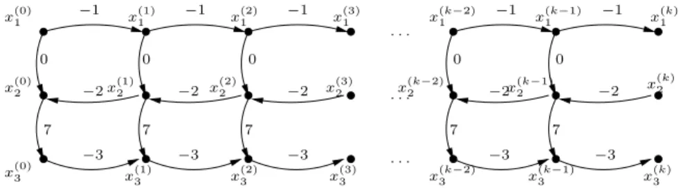
Example 1. Let R(x, x$) be the following DBM relation, where x = {x
1, x2, x3}:
R(x, x$) = x1−x$1≤ −1∧x1−x2≤ 0∧x2−x3≤ 7∧x$2−x2≤ −2∧x3−x$3≤ −3
Figure 1 shows the graph representation of Rk, for k = 1, 2, 3 . . .. By computing
the minimal weight paths in the constraint graph of Rk for k = 1, 2, 3, ... we
obtain, e.g. : R(1)(x, x!) = x1− x2≤ 0 ∧ x1− x3≤ 7 ∧ x2− x3≤ 7 ∧ x1− x!1≤ −1 ∧ x1− x!3≤ 4 ∧ x2− x!3≤ 4 ∧ x3− x!3≤ −3 ∧ x!2− x2≤ −2 ∧ x!2− x3≤ 5 ∧ x!2− x!3≤ 2 R(2)(x, x!) = x1− x2≤ −3 ∧ x1− x3≤ 4 ∧ x2− x3≤ 7 ∧ x1− x!1≤ −2 ∧ x1− x!3≤ −2 ∧ x2− x!3≤ 1 ∧ x3− x!3≤ −6 ∧ x!2− x2≤ −4 ∧ x!2− x3≤ 3 ∧ x!2− x!3≤ −3 R(3)(x, x!) = x1− x2≤ −6 ∧ x1− x3≤ 1 ∧ x2− x3≤ 7 ∧ x1− x!1≤ −3 ∧ x1− x!3≤ −8 ∧ x2− x!3≤ −2 ∧ x3− x!3≤ −9 ∧ x!2− x2≤ −6 ∧ x!2− x3≤ 1 ∧ x!2− x!3≤ −8 R(n≥4)(x, x!) = x1− x2≤ −3 − 3(n − 2) ∧ x1− x3≤ −2 − 3(n − 4) ∧ x2− x3≤ 7 ∧ x1− x!1≤ −n ∧ x1− x!3≤ −14 − 6(n − 4) ∧ x2− x!3≤ 1 − 3(n − 2) ∧ x3− x!3≤ −3n ∧ x!2− x2≤ −2n ∧ x!2− x3≤ 3 − 2(n − 2) ∧ x!2− x!3≤ −3 − 5(n − 2) 2 3
3
Octagonal Constraints
This section is dedicated to octagonal constraints. We provide preliminary results that are needed to define transitive closures of octagonal relations, in the next section.
3 If min
k{x ! y} = −∞ the constraint is logically equivalent to false, and if min{x !
0 7 −1 −1 −1 −1 −1 0 0 0 0 −2 −2 −2 −2 −2 7 7 7 7 −3 −3 −3 −3 −3 . . . . . . x(1)1 x(0)2 x(0)3 x(0)1 x(2)1 x(3)1 x(k−2)1 x(k−1)1 x(k)1 x(1)2 x(2)2 x(k−1)2 x(1)3 x(2)3 x(3)3 x(k−2)3 x(k−1)3 x(k)2 x(k)3 x(3)2 . . .x(k−2)2
Fig. 1. Graph representation of Rk, k = 1, 2, 3, . . .
Definition 7. Let x = (x1, x2, ..., xn) be a set of variables ranging over Z. Then
a formula φ(x) is an octagonal constraint if it is equivalent to a finite conjunction of terms of the form ±xi±xj ≤ αi,j, 2xi≤ βi, or −2xi≤ δi, where αi,j, βi, δi∈ Z
and i (= j, 1 ≤ i, j ≤ n.
The name octagon comes from the fact that, in two dimensions, these con-straints can be graphically represented by polyhedra with at most eight edges. We represent octagons using the set of variables y = (y1, y2, . . . , y2n), with the
convention that y2i−1 stands for xi and y2i for −xi, respectively. For instance,
the octagonal constraint x1+x2= 3 is represented as y1−y4≤ 3∧y2−y3≤ −3.
If we denote by φ = φ[y1/x1, y2/− x1, . . . , y2n−1/xn, y2n/− xn], we obtain
the following valid entailment: φ(x) → (∃y2, y4, . . . , y2n.φ)[x1/y1, . . . , xn/y2n−1].
Moreover φ(x) ↔ (∃y2, y4, . . . , y2n.φ∧&ni=1y2i−1+y2i= 0)[x1/y1, . . . , xn/y2n−1].
To handle the y variables in the following, we define ¯i = i−1, if i is even, and ¯i = i + 1 if i is odd. Obviously, we have ¯¯i = i, for all i ∈ Z, i ≥ 0. The following definition extends the matrix representation from difference bound constraints to octagons:
Definition 8. Let x = (x1, x2, ..., xn) be a set of variables ranging over Z and
φ(x) be an octagonal constraint. Then an octagonal difference bound matrix or octagonal DBM representing φ is an 2n × 2n matrix m such that:
(xi− xj≤ αi,j) ∈ AP (φ) ⇐⇒ m2i−1,2j−1= m2j,2i= αi,j
(−xi− xj ≤ αi,j) ∈ AP (φ) ⇐⇒ m2i,2j−1= m2j,2i−1= αi,j
(−xi+ xj ≤ αi,j) ∈ AP (φ) ⇐⇒ m2i,2j= m2j−1,2i−1 = αi,j
(xi+ xj≤ αi,j) ∈ AP (φ) ⇐⇒ m2i−1,2j= m2j−1,2i= αi,j
(2xi≤ βi) ∈ AP (φ) ⇐⇒ m2i−1,2i= βi
(−2xi≤ δi) ∈ AP (φ) ⇐⇒ m2i,2i−1= δi
A 2n ×2n octagonal DBM m is said to be coherent if and only if mi,j= m¯j,¯i,
for all 1 ≤ i, j ≤ 2n. This property is needed since any constraint xi− xj ≤ α,
1 ≤ i, j ≤ n can be represented as both y2i−1− y2j−1 ≤ α and y2j− y2i≤ α. If
m is coherent, we denote by
the set of concretizations, i.e. the set of models of the octagonal constraint rep-resented by m. Also, m is said to be consistent if γOct(m) (= ∅, and inconsistent
otherwise. The octagonal graph of an octagonal constraint φ(x), represented as a difference bound constraint φ(y) with DBM m, has vertices y, and an arc labeled by mi,j between yi and yj if and only if mi,j<∞, 1 ≤ i, j ≤ 2n.
Definition 9. A consistent coherent 2n × 2n DBM m in Z is said to be tightly closed if and only if the following hold:
1. mi,i= 0 ∀1 ≤ i ≤ 2n
2. mi,¯iis even∀1 ≤ i ≤ 2n
3. mi,j≤ mi,k+ mk,j ∀1 ≤ i, j, k ≤ 2n
4. mi,j≤ (mi,¯i+ m¯j,j)/2 ∀1 ≤ i, j ≤ 2n
The intuition behind the last point is the following: since yi − y¯i ≤ mi,¯i
and y¯j − yj ≤ m¯j,j and yi = −y¯i, yj = −y¯j if we interpret the DBM m as
an octagonal constraint, we have that yi ≤ $ mi,¯i 2 % and −yj ≤ $ m¯j,j 2 %, hence yi− yj ≤ $ mi,¯i 2 % + $ m¯j,j
2 %. Therefore, the tightening of an octagonal DBM has
to come up with values for mi,j that are smaller than $m2i,¯i% + $m2¯j,j%, for all
1 ≤ i, j ≤ 2n.
The tight closure of a 2n × 2n octagonal DBM m is an octagonal DBM m∗ t
such that γOct(m) = γOct(m∗
t), and m∗t is tightly closed. By Theorem 7 in [15],
we know that the tight closure of a consistent octagonal DBM exists and is unique.
We now characterize the consistency of octagonal constraints using their DBM representations. The following result, proved in [2], is crucial for the de-velopments of the next section, therefore we cite (a slightly modified version of) it here:
Theorem 1 ([2]). Let m be a 2n × 2n octagonal DBM consistent and coherent, and let m∗ be its closure. Suppose that'm∗i,¯i
2 ( +'m∗¯i,i 2 ( ≥ 0, for all 1 ≤ i ≤ 2n. Then γOct(m) (= ∅ and the DBM mT defined as:
mTi,j= min ) m∗i,j, *m∗ i,¯i 2 + +*m∗¯j,j 2 +,
for all 1 ≤ i, j ≤ 2n, is the tight closure of m.
It follows immediately that an octagonal constraint is consistent if and only if (1) its constraint graph representation does not contain negative weight cycles and moreover, (2) if the sum between the halved weights of the minimal paths from any node xi to x¯i, and from x¯iand xi is positive. Notice that the lack of
negative weight cycles alone is not enough, as shown by the following example. Example 2. Let φ(x, y, z, x$, y$, z$) = (x − y$ ≤ 1) ∧ (y$+ x ≤ −2) ∧ (−x + z$≤
1) ∧ (−z$− x ≤ 0) be an octagonal constraint on integer variables x, y, z and
has no integer solution. However, its corresponding octagonal DBM does not contain negative weight cycles. The tightening step, i.e. replacing each element mi¯iwith 2
-mi¯i
2
.
, exhibits two negative weight cycles, between +x and −x, and
between +z$ and −z$. 23
We are now ready to give the result of existential quantification over variables occurring within octagons. Namely, we prove that, if φ(x1, . . . , xn) is an
octag-onal constraint, the formula ∃xk.φ, for some 1≤ k ≤ n is again an octagonal
constraint, and its representation is effectively computable from the constraint graph of φ.
In the following, we assume w.l.o.g. that k = n (if this is not the case, we proceed to reindexing variables). From now on assume that φ(x1, . . . , xn) is
consistent, and let m be its 2n × 2n tightly closed coherent octagonal DBM. We denote by β(m) the 2n − 2 × 2n − 2 matrix from which the 2n − 1 and 2n lines and columns have been eliminated. Notice that these correspond to the xn and
−xn terms, respectively.
Lemma 1. Let m ∈ Z2n×2n be the coherent and tightly closed difference bound
matrix for φ(x1, . . . , xn). Then β(m) is also coherent and tightly closed.
The following theorem proves that octagons are closed under existential quan-tification.
Theorem 2. Let x = (x1, x2, . . . , xn) be a set of variables ranging over Z, φ(x)
a consistent octagonal constraint and m the corresponding 2n × 2n octagonal DBM. Then formula ∃xk.φ(x) is equivalent to erasing vertices y2k and y2k−1
together with the incident arcs from the graph G(m∗
t). Moreover, the resulting
graph is also coherent and tightly closed.
4
Octagonal Relations
This section is dedicated to our main result, the definition of the transitive closure of an octagonal relation in Presburger arithmetic. An octagonal relation is defined in a similar way to a difference bound relation.
Definition 10. Let x = (x1, x2, . . . , xn), x$ = (x$1, x$2, . . . , x$n) be sets of
vari-ables ranging over Z. Then an octagonal relation R(x, x$) is a relation that can be
written as a finite conjunction of terms of the form ±xi± xj ≤ ai,j,±x$i± xj≤
bi,j, ±xi ± x$j ≤ ci,j, ±x$i ± x$j ≤ di,j, ±2xi ≤ ei,j or ±2x$i ≤ fi,j, where
ai,j, bi,j, ci,j, di,j, ei,j, fi,j∈ Z and 1 ≤ i, j ≤ n, i (= j.
The DBM and graph representation of an octagonal relation are defined as in the previous case of difference bound relations. For the rest of this section, let R(x, x$) be an octagonal relation and R(y, y$) be its difference bound
represen-tation. Let G be the graph of R, Rk be the k-th iteration of R, mk be its DBM,
and Gk be the graph corresponding to Rk, obtained by connecting k copies of
In order to compute Rk, we need two ingredients. First, we need to check for
consistency of the unfolded relation, that is we need to check that γOct(m k) (= ∅.
Second, we need to obtain the strongest octagonal constraints between y(0) and
y(k) in Gk. By Theorem 2, all intermediate vertices y(l), 0 < l < k can be
eliminated from Gk, and the result is a tightly closed octagonal graph, whose
interpretation is equivalent to Rk.
By Theorem 1, both points require the computation of the values (mk∗)i(l),i(l)
and (mk∗)i(l),i(l), for all 1 ≤ i ≤ 2n and 0 ≤ l ≤ k, where the index i(l) refers to
the variable y(l)
i in the DBM representation of R(y, y$). But these values can now
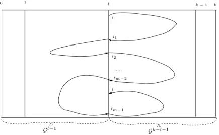
be defined by Presburger formulae, using the results from [7, 6]. To understand this point, consider the situation depicted in Figure 2.
0 1 l k− 1 i ¯ i i1 ... im−2 im−1 k Gl−1 Gk−l−1 i2
Fig. 2. Computing paths of weight (mk∗)i(l),i(l)
Assume in the following that Gkhas no cycles of negative weight. The absence
of negative cycles can be checked a-priori using e.g. the method in [6]. Since we are aiming at computing minimal weight paths, it is sufficient to consider acyclic paths only4. For a fixed 0 < l < k, an acyclic path between the nodes y
i(l) and
y¯i(l), for some 1 ≤ i ≤ 2n, can be decomposed in at most 2n−1 segments starting
and ending in y(l), but not intersecting with y(l), other than in the beginning
and in the end. Moreover, if the path considered is of minimal weight, these segments are of minimal weight as well.
Let 1 ≤ i = i0, i1, . . . , im= ¯i ≤ 2n, be a set of pairwise distinct indices, such that (m∗ k)i(l),i(l)= m−1# j=0 (m∗ k)i(l)j ,i(l)j+1
As in Figure 2, several of the paths y(l)
i ! y (l) i1, y (l) i1 ! y (l) i2, . . . , y (l) im−1 ! y (l) ¯i
will contain only nodes from the set y(≤l), whereas the rest will contain only
nodes from the set y(≥l). Notice that, the paths from y(≤l)connect the terminal
nodes of Gl−1, whereas the paths from y(≥l)connect the initial nodes of Gk−l−1.
Therefore, we have: – (m∗ k)i(l)j ,i(l)j+1= minl−1{y (l) ij !y (l) ij+1}, if y (l) ij !y (l) ij+1 belongs to y (≤l), and – (m∗ k)i(l)j ,i (l) j+1= mink−l−1{y (0) ij !y (0) ij+1}, if y (l) ij !y (l) ij+1 belongs to y (≥l).
But since the minj{x ! y} functions are definable in Presburger arithmetic
[7, 6], we obtain that (m∗
k)i,¯iare Presburger definable as well. Since moreover,
integer division can be defined in Presburger as 'u
2 (
= v ⇐⇒ 2v ≤ u ≤ 2v + 1
it is possible to encode the consistency check of Theorem 1 by a Presburger formula, and effectively perform the check required by Theorem 1:
^ 1≤ i ≤ 2n 0≤ l ≤ k $m∗ i(l),i(l) 2 % + $m∗ i(l),i(l) 2 % ≥ 0
The formula used to check consistency of R(x, x$)k, k ≥ 0 is of size O(22n log 2n),
where n is the number of variables in x. For more details, the interested reader is pointed to [4].
After quantifier elimination, the strongest octagonal relations are obtained by taking the restriction of the tight closure of mk to y(0) and y(k), according
to Theorem 1 and Theorem 2:
yi(0)− yj(k)≤ (m∗kt)i(0),j(k)= min ( (m∗kt)i(0),j(k), $(m∗ kt)i(0),i(0) 2 % + $(m∗ k t)j(k),j(k) 2 %) yi(k)− yj(0)≤ (m∗kt)i(k),j(0) = min ( (m∗kt)i(k),j(0), $(m∗ kt)i(k),i(k) 2 % + $(m∗ k t)j(0),j(0) 2 %) yi(0)− yj(0)≤ (m∗kt)i(0),j(0)= min ( (m∗k t)i(0),j(0), $(m∗ kt)i(0),i(0) 2 % + $(m∗ k t)j(0),j(0) 2 %) yi(k)− yj(k)≤ (m∗kt)i(k),j(k) = min ( (m∗kt)i(k),j(k), $(m∗ k t)i(k),i(k) 2 % + $(m∗ kt)j(k),j(k) 2 %)
Since we showed that all weights of the form m∗
i(l),i(l) are definable in
Pres-burger arithmetic, it follows that Rk is also Presburger definable. Consequently,
the transitive closure of R is the Presburger formula ∃k.Rk, leading to the
fol-lowing theorem:
Theorem 3. The transitive closure of an integer octagonal relation is Pres-burger definable.
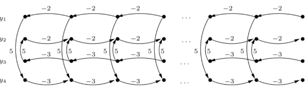
Example 3. Let R(x, x$) be the following octagonal relation, where x = {x 1, x2}
R(x, x$) = x1+ x2≤ 5 ∧ x1$ − x1≤ −2 ∧ x$2− x2≤ −3
Figure 3 shows the graph representation of Rk for k = 1, 2, 3, . . .. The n-step
closure is: Rn(x, x$) = x 1+ x2≤ 5 ∧ x$1− x1≤ −2n ∧ x$2− x2≤ −3n∧ x1+ x$2≤ 5 − 3n ∧ x2+ x$1≤ 5 − 2n ∧ x$1+ x$2≤ 5 − 5n 2 3 . . . . . . . . . . . . y1 y2 y3 y4 −2 −2 −2 −2 −2 −2 −2 −2 −2 −2 −3 −3 −3 −3 −3 −3 −3 −3 −3 −3 5 5 5 5 5 5 5 5 5 5 5 5
Fig. 3. Graph representation of Rk, k = 1, 2, 3, . . .
5
Implementation and Experience
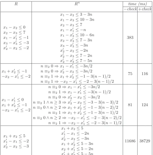
We have implemented the method for computing transitive closures of octagonal relations in a tool for the analysis of counter automata, that we are currently developing. Table 1 shows several octagonal relations (first column), the closed form of their iteration (second column), the execution times (in milliseconds) needed to compute the closed forms without consistency checks (third column), and with consistency checks (fourth column). Notice that the first relation is the difference bound relation example from Section 2, for which no consistency check is needed.
R Rn time (ms) −check +check x1− x2≤ 0 x2− x3≤ 7 x1− x!1≤ −1 x3− x!3≤ −3 x!2− x2≤ −2 x1− x2≤ 3 − 3n x1− x3≤ 10 − 3n x2− x3≤ 7 x1− x!1≤ −n x1− x!3≤ 10 − 6n x2− x!3≤ 7 − 3n x3− x!3≤ −3n x! 2− x2≤ −2n x!2− x3≤ 7 − 2n x! 2− x!3≤ 7 − 5n 383 x1+ x!2≤ −1 −x2− x!1≤ −2 n≡20⇒ x1− x!1≤ −3n/2 n≡20⇒ x!2− x2≤ −3n/2 n≡21⇒ x1+ x!2≤ −1 − 3(n − 1)/2 n≡21⇒ −x2− x!1≤ −2 − 3(n − 1)/2 75 116 x1− x!1≤ 0 x1+ x!2≤ −1 −x2− x!1≤ −2 n≡20⇒ x1− x!1≤ −3n/2 n≡21⇒ x1− x!1≤ −3(n − 1)/2 n≡20⇒ x!2− x2≤ −3n/2 n≡21∧ n ≥ 3 ⇒ x!2− x2≤ −3 − 3(n − 3)/2 n≡20∧ n ≥ 2 ⇒ x1+ x!2≤ −1 − 3(n − 2)/2 n≡21⇒ x1+ x!2≤ −1 − 3(n − 1)/2 n≡20∧ n ≥ 2 ⇒ −x2− x!1≤ −2 − 3(n − 2)/2 n≡21⇒ −x2− x!1≤ −2 − 3(n − 1)/2 81 124 x1+ x2≤ 5 x!1− x1≤ −2 x! 2− x2≤ −3 x1+ x2≤ 5 x!1− x1≤ −2n x!2− x2≤ −3n x1+ x!2≤ 5 − 3n x2+ x!1≤ 5 − 2n x!1+ x!2≤ 5 − 5n 11686 38729
Table 1. Experimental results
The tool, called FLATA, is implemented in Java(TM), and it is currently
available at [10]. The execution times from Table 1 are relative to a Intel(R)
Xeon(TM)CPU 3.00GHz equipped with 1 Gb of RAM. As an approximate upper
bound, we can in principle handle difference bound relations on ten counters, and/or octagons on five counters, within reasonable execution times (≈ 10 min). The fourth example from Table 1 takes significantly more time than the previous ones. This happens because in the pre-processing step we need to replace x1+ x2≤ 5 with x1− x3$ ≤ 5 ∧ x$3+ x2 ≤ 0, where x3 is a fresh variable, thus
having to deal with a DBM relation with 6 counters.
6
Conclusions
We have considered the problem of computing transitive closures of octagonal relations, which are finite conjunctions of atomic formulae of the form ±x±y ≤ c,
where x and y are possibly primed integer variables. We show that the k-th itera-tion of such a relaitera-tion has a Presburger definable closed form. As a consequence, the transitive closure is also Presburger definable. This result enlarges the class of non-deterministic counter automata for which the reachability problem is de-cidable, to counter automata with octagonal transition relations. This result is expected to have an impact in the fields of software verification, as abstract mod-els of software systems are described using octagons. We have implemented our method in a tool for the analysis of counter automata, and report on a number of experiments.
References
1. R. Bagnara. Data-Flow Analysis for Constraint Logic-Based Languages. Ph. D. Thesis, Dipartimento di Informatica, Universit`a di Pisa, 1997.
2. Roberto Bagnara, Patricia M. Hill, and Enea Zaffanella. An improved tight closure algorithm for integer octagonal constraints. In VMCAI, 2008.
3. B. Boigelot. On iterating linear transformations over recognizable sets of integers. TCS, 309(2):413–468, 2003.
4. Marius Bozga, Codruta Girlea, and Radu Iosif. Iterating octagons. TR VERIMAG, 2008.
5. Marius Bozga, Peter Habermehl, Radu Iosif, and Tomas Vojnar. A logic of singly indexed arrays. In LPAR, LNAI 5330, pages 558–573, Springer-Verlag. 2008 6. Marius Bozga, Radu Iosif, and Yassine Lakhnech. Flat parametric counter
au-tomata. In ICALP, LNCS 4052, pages 577–588. Springer-Verlag, 2006.
7. Hubert Comon and Yan Jurski. Multiple counters automata, safety analysis and presburger arithmetic. In CAV, LNCS 1427, pages 268–279, 1998.
8. Patrick Cousot and Nicolas Halbwachs. Automatic discovery of linear restraints among variables of a program. In POPL, pages 84–97. ACM Press, 1978.
9. A. Finkel and J. Leroux. How to compose presburger-accelerations: Applications to broadcast protocols. In Proc. FST&TCS, LNCS 2556, pages 145–156, Springer-Verlag, 2002.
10. http://www-verimag.imag.fr/˜async/flata/flata.html.
11. Peter Habermehl, Radu Iosif, and Tomas Vojnar. What else is decidable about integer arrays? In FOSSACS, LNCS 4962, pages 474–489, 2008.
12. Warwick Harvey and Peter Stuckey. A unit two variable per inequality integer constraint solver for constraint logic programming. In Australian Computer Science Conference, pages 102–111, 1997.
13. O. H. Ibarra. Reversal-bounded multicounter machines and their decision prob-lems. Journal of the ACM, 25(1):116–133, 1978.
14. J. Leroux and G. Sutre. Flat counter automata almost everywhere! In ATVA, LNCS 3707, pages 489–503. Springer-Verlag, 2005.
15. A. Min´e. The octagon abstract domain. Higher-Order and Symbolic Computation, 19(1):31–100, 2006.
16. M. Minsky. Computation: Finite and Infinite Machines. Prentice-Hall, 1967. 17. M. Presburger. ¨Uber die Vollstandigkeit eines gewissen Systems der Arithmetik.
Comptes rendus du I Congr´es des Pays Slaves, Warsaw 1929.
18. C. Reutenauer. Aspects Math´ematiques des R´eseaux de Petri. Collection ´Etudes et Recherches en Informatique. Masson, 1989.