Classical simulation complexity of restricted
models of quantum computation
by
Dax Enshan Koh
B.S., Stanford University (2011)
M.Sc., University of Waterloo (2013)
Submitted to the Department of Mathematics
in partial fulfillment of the requirements for the degree of
Doctor of Philosophy
at the
MASSACHUSETTS INSTITUTE OF TECHNOLOGY
June 2019
@
Massachusetts Institute of Technology 2019. All rights reserved.
Signature
redacted
A uthor ...
Department of Mathematics
Certified by...
Accepted by
MASSACUSTS INSTITUTE OF TECHNOWDGYJUN 0 5 2019
LIBRARIES
/M~ay 3, 2019
/Signature redacted
...
Peter W. Shor
Morss Professor of Applied Mathematics
Thesis Supervisor
Signature redacted,
Jonathan Kelner
Chairman, Department Committee on Graduate Theses
Classical simulation complexity of restricted models of
quantum computation
by
Dax Enshan Koh
Submitted to the Department of Mathematics on May 3, 2019, in partial fulfillment of the
requirements for the degree of Doctor of Philosophy
Abstract
Restricted models of quantum computation are mathematical models which describe quantum computers that have limited access to certain resources. Well-known ex-amples of such models include the boson sampling model, extended Clifford circuits, and instantaneous quantum polynomial-time circuits. While unlikely to be universal for quantum computation, several of these models appear to be able to outperform classical computers at certain computational tasks, such as sampling from certain probability distributions. Understanding which of these models are capable of per-forming such tasks and characterizing the classical simulation complexity of these models-i.e. how hard it is to simulate these models on a classical computer-are some of the central questions we address in this thesis.
Our first contribution is a classification of various extended Clifford circuits ac-cording to their classical simulation complexity. Among these circuits are the conju-gated Clifford circuits, which we prove cannot be efficiently classically simulated up to multiplicative or additive error, under certain plausible conjectures in computational complexity theory. Our second contribution is an estimate of the number of qubits needed in various restricted quantum computation models in order for them to be able to demonstrate quantum computational supremacy. Our estimate is obtained by fine-graining existing hardness results for these restricted models. Our third contribution is a new alternative proof of the Gottesman-Knill theorem, which states that Clif-ford circuits can be efficiently simulated by a classical computer. Our proof uses the sum-over-paths technique and establishes a correspondence between quantum circuits and a class of exponential sums. Our final contribution is a theorem characterizing the operations that can be efficiently simulated using a particular rebit simulator. An application of this result is a generalization of the Gottesman-Knill theorem that allows for the efficient classical simulation of certain nonlinear operations.
Thesis Supervisor: Peter W. Shor
Acknowledgments
I would like to express my deep gratitude to my thesis supervisor Peter W. Shor for
his unconditional support, encouragement and guidance throughout my time at MIT. Peter's creativity and mastery of the field has been a source of great inspiration for me.
I would like to thank my co-authors for their time, ideas and our many fruit-ful discussions: Scott Aaronson, Jacob D. Biamonte, Adam Bouland, Kaifeng Bu, Alexander M. Dalzell, Joseph F. Fitzsimons, Aram W. Harrow, Rolando L. La Placa, Zi-Wen Liu, Mauro E.S. Morales, Murphy Yuezhen Niu, Mark D. Penney, Christo-pher Perry, Robert W. Spekkens, Theodore J. Yoder, and Yechao Zhu. I have learned much from our collaborations. In addition, I would like to thank Mason Biamonte, Siong Thye Goh, Anand Natarajan, Hakop Pashayan, and many others with whom I have had many insightful discussions.
I have been fortunate to have had the opportunity to visit and collaborate with
various research groups around the world. I would like to thank Huangjun Zhu, Robert Spekkens, and Beni Yoshida for hosting me on multiple visits to the Perimeter Institute for Theoretical Physics; Si-Hui Tan and Joseph Fitzsimons for hosting me at the Singapore University of Technology and Design; Hakop Pashayan and Stephen Bartlett for hosting me at the University of Sydney; Man-Hong Yung for hosting me at the Southern University of Science and Technology in Shenzhen; Alexander Rivosh and Andris Ambainis for hosting me at the University of Latvia; and Dirk Oliver Theis for hosting me at the University of Tartu. I would also like to thank Jacob D. Biamonte and the Deep Quantum Labs at the Skolkovo Institute of Science and Technology for hosting me as a research intern during the summer of 2018, and MISTI-Russia for making this possible.
I would like to thank members of my Thesis Examination Committee-Peter W.
Shor, Michel X. Goemans, and Aram W. Harrow-for generously agreeing to oversee my thesis defense and for useful comments on this thesis. Also, I would like to thank members of my Qualifying Examination Committee-Peter W. Shor, Hung
Cheng, and Robert G. Gallager-for providing useful feedback during my qualifying examination.
I would like to acknowledge funding support from the National Science Scholarship
awarded by the Agency for Science, Technology and Research (A*STAR), Singapore, as well as the Enabling Practical-scale Quantum Computing (EPiQC) Expedition, an
NSF expedition in computing.
Last but not least, I would like to thank my family for their unwavering support and encouragement.
Contents
1 Introduction
1.1 M otivation . . . . 1.2 Organization and summary of results . . . .
2 Preliminaries
2.1 Notational guide . . . . 2.2 Quantum states, transformations and measurements .
2.3 Quantum circuits . . . . 2.3.1 Examples of quantum gates . . . .
2.3.2 Universality . . . . 2.4 Pauli group . . . . 2.4.1 Properties of the Pauli group . . . . 2.4.2 F2 representation of the Pauli group . . . .
2.5 Clifford group . . . . 2.5.1 Elements of the Clifford group . . . .
2.6 Classical and quantum computational complexity thec
2.6.1 P, NP and the polynomial hierarchy . . . .
2.6.2 Complexity of counting . . . .
2.6.3 Space complexity . . . . 2.6.4 Classical randomized complexity . . . .
2.6.5 Bounded-error quantum polynomial time . . . 2.6.6 Postselection . . . .
2.7 Notions of classical simulation of quantum computation
23 23 27 31 . . . . 31 . . . . 32 . . . . 34 . . . . 35 . . . . 38 . . . . 39 . . . . 39 . . . . 41 . . . . 43 . . . . 45 . . . . 50 . . . . 51 . . . . 54 . . . . 55 . . . . 56 . . . . 58 . . . . 60 62 ry
2.8 Restricted models of quantum computation . . . .
2.8.1 Clifford circuits . . . .
2.8.2 Instantaneous quantum polynomial-time circuits .
2.8.3 Depth-one QAOA circuits . . . . 2.8.4 DQC1 circuits . . . . 2.8.5 Boson sampling model . . . .
nded 66 . 66 . 68 . 69 . 73 73
Clifford circuits and their classical simulation complexi-3 Exte ties 3.1 3.2 3.3 3.4 3.5 M otivation . . . . Preliminary definitions and notations . . . . Notions of classical simulation . . . . Results and discussion . . . . Proofs of main theorems . . . .
3.5.1 Rules for proving results in Table 3.1 . . . .
3.5.2 Proof of Theorem 39: Strong(n) simulation of nonadaptive Clif-ford circuits with product inputs and computational basis outputs
3.5.3 Proof of Theorem 40: Strong(n) simulation of adaptive Clifford circuits with computational basis inputs and outputs . . . . . 3.5.4 Proof of Theorem 46: Weak simulation of nonadaptive Clifford circuits with computational basis inputs and product outputs
3.5.5 Proof of Theorem 48: Strong(n) simulation of nonadaptive Clif-ford circuits with product inputs and computational basis outputs
3.5.6 Proof of Theorem 49: Strong(1) simulation of nonadaptive Clif-ford circuits with product inputs and outputs . . . .
3.5.7 Proof of Theorem 50: Weak(1) simulation of adaptive Clifford circuits with computational basis inputs and product outputs
3.5.8 Constructing circuits for 3-CNF formulas . . . . 3.5.9 Constructing C . . . . 3.5.10 Constructing Qf . . . . 77 78 80 84 86 89 89 90 93 95 98 99 100 101 102 105
3.6 Concluding remarks . . . . 106
4 Conjugated Clifford circuits 107 4.1 Overview of results . . . . 107
4.1.1 Proof techniques . . . . 110
4.1.2 Relation to other works on modified Clifford circuits . . . . . 113
4.2 Conjugated Clifford circuits . . . . 114
4.2.1 Postselection gadgets . . . . 115
4.3 Weak simulation of CCCs with multiplicative error . . . . 117
4.3.1 Classification results . . . . 117
4.3.2 Proofs of efficient classical simulation . . . . 120
4.3.3 Proofs of hardness . . . . 121
4.4 Weak simulation of CCCs with additive error . . . . 127
4.5 Evidence in favor of hardness conjecture . . . . 131
4.6 CCCs and other notions of simulation . . . . 134
4.7 Measurement-based quantum computing proof of multiplicative hard-ness for CCCs for certain U's . . . . 136
4.8 Open Problem s . . . . 146
5 How many qubits to reach quantum supremacy? 149 5.1 Motivation and outline of results . . . . 150
5.2 Background . . . . 154
5.2.1 Counting complexity and quantum supremacy . . . . 154
5.2.2 Degree-3 polynomials and the problem poly3-NONBALANCED . 157 5.2.3 The permanent and the problem per-int-NONZERO . . . . 159
5.3 Lower Bounds . . . . 161
5.3.1 For IQP Circuits . . . . 161
5.3.2 For QAOA circuits . . . . 162
5.3.3 For boson sampling circuits . . . . 165
5.3.4 Evidence for conjectures . . . . 166
5.4
5.5 5.6
Reduction from poly3-NONBALANCED to per-int-NONZERO . . . . 174
Better-than-brute-force solution to poly3-NONBALANCED . . . . 178
Concluding remarks . . . . 180
6 Computing quopit Clifford circuit amplitudes by the sum-over-paths technique 183 6.1 Motivation and outline of results ... 184
6.2 Preliminary definitions and notation ... ... 186
6.3 Constructing sum-over-paths expressions for quopit Clifford circuits . 188 6.4 Evaluating the sum over paths . . . . 190
6.4.1 Step 1: Diagonalizing 0 . . . . 190
6.4.2 Step 2: Using the exponential sum formula . . . . 191
6.4.3 Running time . . . . 193
6.4.4 Proof of Theorem 84 . . . . 193
6.5 Balancedness of quopit Clifford circuits . . . . 197
7 Classical simulation of quantum circuits by half Gauss sums 201 7.1 Outline of results . . . . 202
7.2 Half Gauss sums . . . . 7.2.1 Univariate case . . . . 7.2.2 Multivariate case . . . . 7.3 m-qudit Clifford circuits . . . . 7.4 Hardness results and complexity dichotomy theorems 7.4.1 Degree-3 polynomials . . . . 7.4.2 Without the periodicity condition . . . . 7.4.3 Other incomplete Gauss sums . . . . 7.4.4 Complexity dichotomy theorems . . . . 7.5 Tractable signatures in Holant problems . . . . 7.6 Appendix for Chapter 7 . . . . 7.6.1 Exponential sum terminology . . . . 7.6.2 Properties of Gauss sum . . . . . . . . 204 . . . . 204 . . . 209 . . . 213 . . . 219 . . . 219 . . . . 220 . . . 222 . . . . 223 . . . . 224 . . . . 227 . . . 227 . . . 228
Half Gauss sum for d = -W2d with even d . . . . 229
Relationship between half Gauss sums and zeros of a polynomial230 8 Quantum simulation from the bottom up: the case of rebits 233 8.1 Introduction . . . .. . . . . 8.1.1 Two kinds of simulation . . . . 8.1.2 Simulation using rebits . . . . 8.1.3 Our results . . . . 8.1.4 Related work . . . . 8.1.5 N otation . . . . 8.2 Quantum circuits with rebits . . . . 8.2.1 Rebit encoding and decoding of states . . . . 8.2.2 Rebit encoding and decoding of operators . . . . . 8.2.3 Rebit encoding and decoding of measurements . . . 8.2.4 Bottom-up tomography . . . . 8.3 Partial antiunitarity . . . . 8.3.1 Partial complex conjugation . . . . 8.3.2 Partial antiunitary operators . . . . 8.4 Simulating partial antiunitary operators . . . . 8.4.1 Rebit simulation of unitaries: top-down perspective 8.4.2 Rebit simulation of non-unitaries: bottom-up persp 8.5 Universal gate sets for R-unitaries . . . . 8.6 The R-Clifford hierarchy . . . . 8.7 Discussion and open questions . . . . 8.8 Appendix for Chapter 8 . . . . 8.8.1 A simple motivating example . . . . 8.8.2 8.8.3 8.8.4 8.8.5 . . . 234 . . . 236 . . . 238 . . . . 239 . . . 245 . . . . 246 . . . . 247 . . . . 247 . . . . 249 . . . . 257 . . . . 260 . . . . 262 . . . . 262 . . . . 264 . . . 276 . . . 276 ective Complex conjugation as a Gottesman-Knill simulation R-linear operators . . . . The ring of R-linear operators: algebraic properties . . Equivalent expressions for the rebit encoding of a linear 279 284 293 302 305 305 . . . . 306 . . . . 308 . . . . 309 operator312 7.6.3 7.6.4
Equivalence of norm definitions . . . .
Alternative formulation of Theorem 126 . . On orthogonal projections . . . .
Matrix representation of R-linear operators .
Proof of Lemma 162 . . . . Pauli sets with different allowed phases . . .
. . . 313 . . . 314 . . . 315 . . . 316 . . . 319 . . . 321 A Characterizations of the Clifford group
A.1 The single-qubit case . . . . A.2 The multi-qubit case . . . . A.3 Enumerating the Clifford group . . . . References 8.8.6 8.8.7 8.8.8 8.8.9 8.8.10 8.8.11 327 335 340 349 354
List of Figures
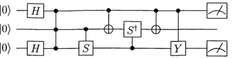
2-1 Example of a quantum circuit, represented as a quantum circuit
dia-gram. The sequence of gates in the circuit may be written as CY13CX12
CSt2CX12CS23CCZ 23HjH3. We write Gi to mean that the gate G
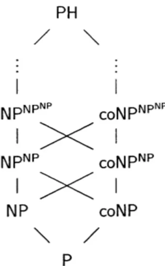
acts on the ith qubit. . . . . 34 2-2 Hasse diagram representing the poset
(X,
5), where X comprises PHand all its levels. We write A < B if the statement that A C B is
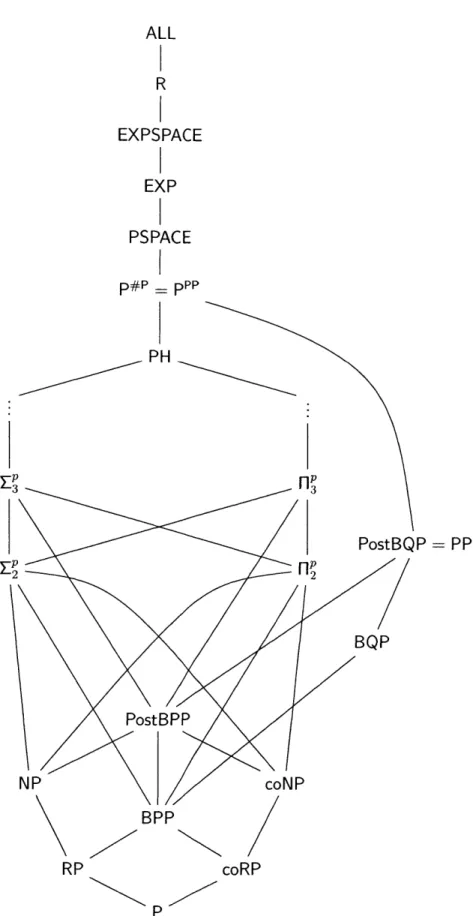
known to be true at the time of writing. . . . . 53 2-3 Hasse diagram representing the known subset relations
(C)
betweenthe various classes introduced in Chapter 2.6. . . . . 63 3-1 Circuit diagram for the Clifford computational tasks considered in this
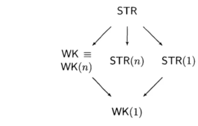
chap-ter. The gates V and Ut are arbitrary single qubit unitaries, B is a Clifford circuit, the input state is the all-zero computational basis state, and the output measurement is performed in the computational basis. . . . . 82 3-2 Relationships between different notions of classical simulation of
Clif-ford computational tasks. An arrow from A to B
(A
-4 B) meansthat an efficient A-simulation of a computational task implies that there is an efficient B-simulation for the same task. The statement
WK = WK(n) is shorthand for WK -+ WK(n) and WK(n) - WK. . . 85
3-3 Uncomputation trick, in which the output bits, except for those in the target register, are reset to their input values. The state evolves as
fol-lows: (x, 1,..., 1, 0) -+ (f(x), j 2, . . ., ja(N), 0) > (f(X)j2, -.- , a(N), f(X))
4-1 Relationships between different notions of classical simulation and summary of the hardness of simulating CCCs. An arrow from A to B (A -+ B)
means that an efficient A-simulation of a computational task implies that there is an efficient B-simulation for the same task. Note also that an weak(n) simulation exists if and only if a weak simulation exists. For a proof of these relationships, see Chapter 3.3. The two curves indicate the boundary between efficiencies of simulation of U-CCCs, where U is not a Clifford operation times a Z rotation. "Hard" means that an efficient simulation of U-CCCs is not possible, unless PH collapses. "Conjectured hard" means that an efficient simulation of U-CCCs is not possible, if we assume Conjecture 69. "Easy" means that an efficient simulation of U-CCCs exists. Note that when U is a Clifford operation times a Z rotation, all the above notions become easy . . . . 135
5-1 IQP circuit Cf corresponding to the degree-3 polynomial f(z) = zi + z2 + z1z2 + z1z2z3. The unitary Uf implemented by the circuit has the
property that (0 Uf |0) = gap(f)/2" where in this case n = 3. .. .. 158
5-2 Gadget that uses an ancilla qubit to implement the H gate within
the QAOA framework. Here the gate
Q
is the diagonal two-qubit gatediag(1, i, 1, -1) which can be written as exp(-iz(6 1)(01 + 2|11)(111)).
Thus, it can be implemented by adding 8 constraints to the constraint
Hamiltonian C. The H gate is implemented by applying the
5-3 Gadget for each term in the degree-3 polynomial
f.
Unlabeled edges are assumed to have weight 1. The three dashed lines are connected via the XOR gadget to the dashed lines in the variable gadgets for the variables that appear in the term, as exemplified by the labeling of vertices v and v' in the context of Figure 5-5. If all three variables are true, the term gadget will contribute a cycle cover factor of -1, excluding the factors of 4 from dotted edges. If at least one variable is false, the term will contribute a cycle cover factor of 1. . . . . 1765-4 Gadget for each variable in the degree-3 polynomial
f.
The number of dashed lines is equal to the number of terms in which the variable appears, so this example is for a variable that appears in four terms. The dashed lines are connected to the dashed lines in the term gadget in which that variable appears via the XOR gadget, as exemplified by the labeling of vertices u and u' in the context of Figure 5-5. . . . . . 176 5-5 XOR gadget that connects dotted lines from node u to u' in the variablegadget with dotted lines from node v to v' in the term gadget. The effect of the XOR gadget is that any cycle cover must use either the edge from u to u' or the edge from v to v', but not both. Each XOR
gadget contributes a factor of 4 to the weight of the cycle cover. . . . 177
6-1 Example of a quopit Clifford circuit. As explained in the text, we can assume
without loss of generality that each register ends in a Fourier gate. . . . . 189 6-2 Labeled circuit corresponding to the circuit in Figure 6-1. The phase
poly-nomial is read off to be S(Xi, X2, X3) = a2X1 + a3X2 + aiX3 + X3bi + b2(ai +
X1) + b3(a1 + x, + X2) + 2-ai(a - 1). . . . . 189
8-1 Commutative diagram illustrating the relationships between the sets
8-2 Diagram illustrating the relationships between different classes of
op-erators considered in this chapter. A line from A to B (where A is higher than B) means that A is a proper superset of B. The ellipses represent the infinite towers of classes corresponding to different levels of the respective Clifford hierarchies. . . . . 241
8-3 The proof of 2-locality of rebit tomography using H, CZ, and
single-rebit computational basis measurements. (a) Measuring Z, (b) Mea-suring X, and (c) MeaMea-suring Y 0 Y. . . . . 261
8-4 Compiling an orthogonal Clifford circuit on n qubits. The top line represents 1 qubit while the bottom represents n - 1 qubits. . . . . . 302 8-5 The circuit, built from only orthogonal gates, implementing a C"-V
gate with two controls (the top two qubits), corresponding to n = 3. Further controls are added in the natural way, extending the CZ and
List of Tables
2.1 A complete list of all 24 elements of the single-qubit Clifford group
C1
/U(1),
written as products of H, S, X = HS2H and Z = S2.The rows are indexed by permutations - on
{1,
2, 3} written incy-cle notation and the columns are indexed by a, -y {+, -}. The
in-tegers ijk E {1, 2, 3}3, with distinct i,
j,k,
are defined by i = o-(1),j
= o(2) and k = a-(3). The Clifford operator U corresponding to i,j,k
E {1,2,3} and a,-y E {+,-} is the unique U satisfyingUXUt = auo and UZUt = 7-k. The symbol in parenthesis (p),
where / E
{+,
-}, written below the Clifford operator U is defined byUYUt = 3uo. For example, the entry HS with row index ijk = 231,
column index a-y = -+ and 3 = - means that U = HS satisfies
UXUt = -O-2 = -Y, UYUf = -O-3 = -Z and UZUt o- = X. . 49
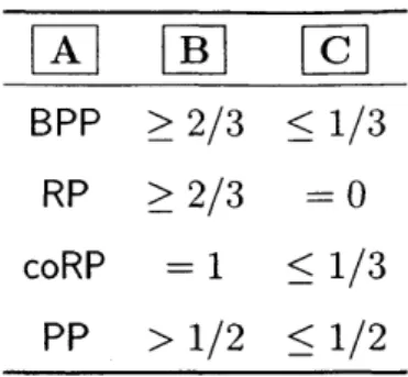
2.2 Definitions of BPP, RP, coRP and PP, obtained by replacing the place-holders A, B and C in Template 14 with those in the table. . . . . . 57
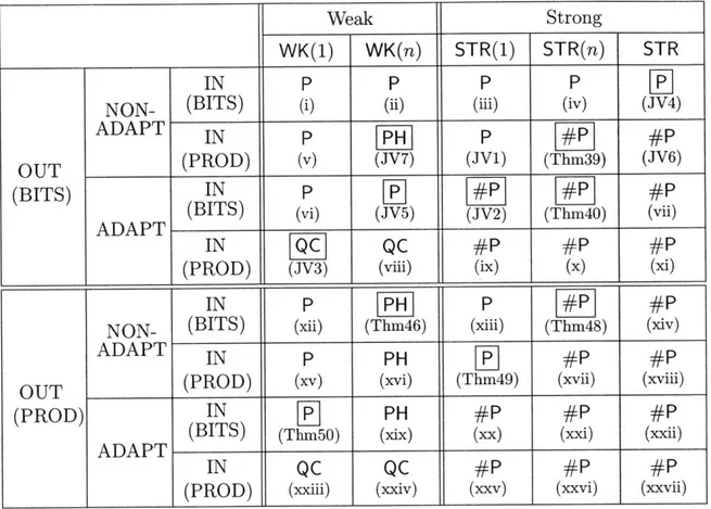
3.1 Classification of the classical simulation complexities of families of Clifford circuits with different ingredients. P stands for efficiently classically simula-ble. #P stands for #P-hard. QC stands for QC-hard and PH stands for "if efficiently classically simulable, then the polynomial hierarchy collapses". The proofs of JV 1-7 can be found in [143]. Theorems 39-50 are about cases not found in [143] and are the main results of this chapter. (i)-(xxvii) are results that follow immediately from these theorems by using the rules in Chapter 3.5.1. The 11 cases with boxed symbols are the core theorems, from which all other cases can be deduced using rules which we describe in Chapter 3.5.1. These include all the main theorems JV 1-7 and Theorems
39-50, except JV1 and JV6, which turn out to be special cases of Theorem
49 and Theorem 39 respectively. . . . . 87
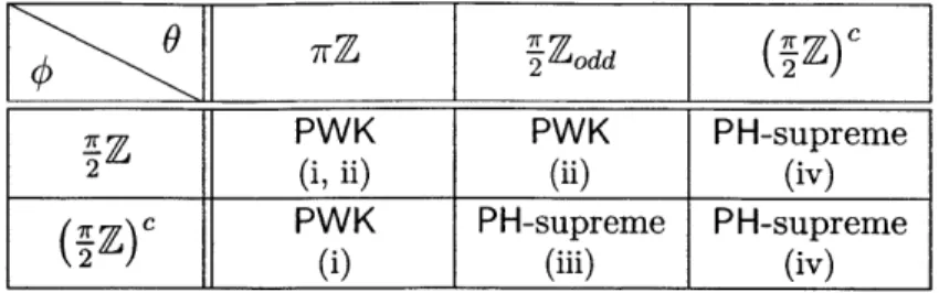
4.1 Complete complexity classification of U-CCCs (where U = Rz(O)R2(O))
with respect to weak simulation, as we vary # and 6. The roman numer-als in parentheses indicate the parts of Lemma 57 that are relevant to the corresponding box. All U-CCCs are either in PWK (i.e. can be efficiently simulated in the weak sense) or PH-supreme (i.e. cannot be simulated effi-ciently in the weak sense, unless the polynomial hierarchy collapses.)
. . . . . . . . . . . .. . . . . ..118
7.1 Hardness of computing Z1/2k(2,
f),
where k > 0 or k > 1, and f is apolynomial function with coefficients in Z and domain Z'. Here, 'periodic' means that
f satisfies the periodicity condition (7.3), and 'aperiodic' means
thatf does not necessarily satisfy it. The label FP means that
Zl/2k(d,f)
can be computed in classical polynomial time, and #P-hard means that there is no efficient classical algorithm to compute ZI/2k(d,f),
unless the widely-believed conjecture FP f #P is false. . . . . 203A. 1 Number of elements in the n-qubit Clifford group IC,/U(1) and the
group of n-qubit operators generated by H, S, CZ, for n = 1, 2,...,6.
The cardinalities of these groups are related by lCn = IC,/U(1)1 =
11(H, S, CZ)nI. The sequence I(H, S, CZ)"I is recorded as sequence A003956 in the On-Line Encyclopedia of Integer Sequences (OEIS)
List of Publications
This thesis is based on the following publications and preprints:
1. Dax Enshan Koh, "Further extensions of Clifford circuits and their
classi-cal simulation complexities," Quantum Inf. Comput. 17, 0262-0282 (2017). arXiv:1512.07892. ECCC TR16-004.
2. Dax Enshan Koh, Mark D. Penney, and Robert W. Spekkens, "Computing quopit Clifford circuit amplitudes by the sum-over-paths technique," Quantum Inf. Comput. 17, 1081-1095 (2017). arXiv:1702.03316.
3. Dax Enshan Koh, Murphy Yuezhen Niu, and Theodore J. Yoder, "Quantum
simulation from the bottom up: the case of rebits," J. Phys. A: Math. Theor.
51, 195302 (2018). arXiv:1708.09355.
4. Adam Bouland, Joseph F. Fitzsimons, and Dax Enshan Koh, "Complexity Clas-sification of Conjugated Clifford Circuits." In: 33rd Computational Complex-ity Conference (CCC 2018), R. A. Servedio, ed., vol. 102 of Leibniz Interna-tional Proceedings in Informatics (LIPIcs), Dagstuhl, Germany, pp. 21:1-21:25, Schloss Dagstuhl-Leibniz-Zentrum fuer Informatik (2018). arXiv:1709.01805.
5. Alexander M. Dalzell, Aram W. Harrow, Dax Enshan Koh, and Rolando L. La
Placa, "How many qubits are needed for quantum computational supremacy?"
arXiv:1805.05224 (2018).
6. Kaifeng Bu and Dax Enshan Koh, "Classical simulation of quantum circuits by
Other publications and preprints that I contributed to during my PhD:
1. Zi-Wen Liu, Christopher Perry, Yechao Zhu, Dax Enshan Koh, and Scott
Aaron-son, "Doubly infinite separation of quantum information and communication," Phys. Rev. A 93, 012347 (2016). arXiv:1507.03546. ECCC TR16-016.
2. Mark D. Penney, Dax Enshan Koh, and Robert W. Spekkens, "Quantum circuit dynamics via path integrals: Is there a classical action for discrete-time paths?" New J. Phys. 19, 073006 (2017). arXiv:1604.07452.
3. Jacob D. Biamonte, Mauro E. S. Morales, and Dax Enshan Koh, "Quantum
Supremacy Lower Bounds by Entanglement Scaling." arXiv:1808.00460 (2018). 4. Kaifeng Bu and Dax Enshan Koh, "Efficient classical simulation of Clifford
Chapter 1
Introduction
1.1
Motivation
Quantum computers, which were first proposed in the 1980s by Manin [164], Feynman [102], and others, promise to offer significant computational benefits compared to to-day's classical computers. This promise has been driven by the discovery of quantum algorithms designed to be run on quantum computers, which can potentially solve certain problems much faster than the best classical algorithms possible. A famous example of such a quantum algorithm is due to Shor [205,207], whose eponymous al-gorithm can solve the factoring problem exponentially faster than the fastest classical algorithms we know today. Since Shor's discovery, several other quantum algorithms have been discovered [171]. For a comprehensive catalog of quantum algorithms, we refer the reader to the Quantum Algorithm Zoo [141], which at the time of writing contains about 60 quantum algorithms.
While significant progress has been made in the field of quantum algorithms, fast quantum algorithms alone are obviously not sufficient to provide convincing evidence that quantum computers would offer benefits compared to their classical counterparts. Two additional ingredients are needed. The first ingredient is experimental: we need to build quantum computers that are capable of running these quantum algorithms; otherwise, any advantage that these quantum algorithms possess cannot be actualized. The second ingredient is theoretical: we need to prove that the quantum algorithms
we design indeed provide a speedup (or offer some other advantage) over all possible classical algorithms for the same problem. While considerable progress has been made in developing these experimental and theoretical ingredients, the challenges faced remain large and attempts to address them continue to be active areas of research.
On the experimental front, one of the central challenges is that building a quantum computer is difficult. On the one hand, in order to use a quantum system as a quantum computer, we need to isolate it from the outside world. This is because quantum systems that are not perfectly isolated from the environment undergo decoherence and lose information to the environment [20,140]. On the other hand, we need to be able to control the quantum system from the outside to allow inputs to be fed into the computer, and be able to read out the results of the measurements. This trade-off between the above requirements presents opposing design challenges to building quantum computers [189].
On the theoretical front, one of the main challenges is that proofs of compu-tational hardness are notoriously difficult to establish-consider, for example, the long-standing P NP problem [4, 70]. We do not have a theoretical proof yet of
any quantum algorithm that can outperform the best classical algorithm for a given task, in the standard paradigm of polynomial-versus-exponential running time, in a computational complexity setting. For example, even though Shor's algorithm out-performs all known classical factoring algorithms, there is no provable guarantee that future yet-to-be-discovered classical factoring algorithms will not be able to match the performance of Shor's algorithm. More generally, the question of whether the complexity classes BPP (the class of problems that can be efficiently solved with a classical randomized algorithm) and BQP (the class of problems that can be efficiently solved with a quantum algorithm) are equal remains open. Proving that these two classes are not equal would be a momentous breakthrough, not only because it would prove that quantum computers are exponentially more powerful than classical ones, but also because it would resolve major unsolved problems in classical computational complexity theory; for example, it would prove the long-standing conjecture that
While a complete solution to the above experimental and theoretical challenges has yet to be found, progress has been made towards addressing them. On the exper-imental front, after years of research and development in fabrication and materials, the first quantum computers that might be able to outperform state-of-the-art clas-sical computers are now in the pipeline. For example, Google announced last year that it had built Bristlecone, a 72-qubit quantum computer based on superconduct-ing circuits [144]. We are now entersuperconduct-ing a pivotal era in quantum technology, which has been dubbed the Noisy Intermediate-Scale Quantum (NISQ) era [189]. Here, "noisy" emphasizes that experimentalists will likely have only imperfect control over the qubits in the quantum computer, and "intermediate-scale" refers to the size of near-term quantum computers, which are likely to be able to handle only between 50
and a few hundred qubits.
On the theoretical front, even though a proof of an unconditional separation be-tween BPP and BQP remains out of reach, it has been possible to prove quantum-classical separations under additional conditions or assumptions. Popular approaches include proving separations in the black box model, or proving separations between restricted quantum computers and restricted classical computers. An example of a result using the former approach is an oracle separation1 between BQP and BPP [29]. An example of a result using the latter approach is a separation between constant-depth quantum circuits and constant-constant-depth classical circuits [43]. A third popular approach is to prove separations based on plausible complexity assumptions. Results of this type typically involve choosing a widely-believed conjecture C and a task T for which we can prove the following: (i) T can be performed efficiently on a quantum computer, (ii) If T can also be performed efficiently on a classical computer, then C is false. In other words, the plausibility of C gives evidence that quantum computers outperform classical computers. Examples of such results include theorems showing that quantum computers are able to efficiently perform sampling tasks that classi-cal computers cannot, under the assumption that the polynomial hierarchy does not
'More recent results have generalized this to an oracle separation between BQP and MA [226], and an oracle separation between BQP and PH [193].
collapse [5, 48,97].
In light of the above experimental and theoretical advances, a question that has been frequently asked is: when can we expect to observe an empirical demonstration of a quantum advantage that is strongly supported by plausible theoretical assumptions? Performing such a demonstration would be a critical milestone in the development of quantum computers and the first step towards useful quantum computation. It would show what has come to be called 'quantum supremacy' [188] (or alternatively, 'quantum computational supremacy' [123]), a term which has recently come into vogue to describe such a demonstration of a quantum advantage, whose goal is to overturn the Extended Church-Turing Thesis [184, 238] as confidently as possible. Due to the recent developments of near-term quantum devices, there are expectations that quantum supremacy could be achieved in the next few years.
The potential imminence of quantum supremacy has sparked interest in under-standing which quantum computational models are both (i) potentially realizable in the near term and (ii) capable of solving classically-hard problems. Models satis-fying (i) are likely to not be capable of arbitrary universal quantum computation, but instead be limited by restrictions of some kind. We shall use the term restricted
models of quantum computation to refer to quantum computers that have limited
access to certain resources. Some examples of restricted quantum computing models include extended Clifford circuits [143,148], boson sampling circuits [5] and instan-taneous quantum polynomial time (IQP) circuits [48]. Because these models are not likely to require the full power of quantum computation, they are potentially easier to implement in the laboratory and are therefore conceivably good candidates for implementation in the near term. The remaining question, then, is whether these various restricted models also satisfy (ii), i.e. can they solve problems which are hard for classical computers? If not, can we show that these models can be efficiently simulated on a classical computer? Studying the classical simulation complexities of these restricted models-i.e. how hard it is to classically simulate these models-is one of the central questions we will address in this thesis.
models is useful not just in helping us to understand which models might be useful candidates for demonstrating quantum supremacy; it also yields useful insights on the relationship between quantum and classical computational power and helps us understand the origin of quantum speedup (if it exists), the reason why quantum supremacy could exist in the first place. To see this, suppose that we start with a restricted model that is efficiently classically simulable. If adding certain ingredients to the restricted model creates a new model that is hard to simulate classically, then we could regard those ingredients as an essential 'resource' for quantum computational power. In this thesis, we will see several examples of how adding ingredients to a restricted model of quantum computation changes its classical simulation complexity. In the preceding paragraphs, we gave an overview of some of the main challenges and advances in the field of quantum computation, and motivated some of the broad questions that this thesis addresses. In the next section, we will elaborate on some of these questions, and summarize the main results and contributions of this thesis.
1.2
Organization and summary of results
This thesis is organized as follows. In Chapter 2, we introduce some of the ba-sic definitions, notation and tools used in quantum computation and computational complexity theory. We describe various restricted models of quantum computation, and summarize some of their properties. An example of a restricted model we will discuss is the class of Clifford circuits, which has important applications in many subfields of quantum computation. An important result about Clifford circuits is the Gottesman-Knill Theorem, which states that Clifford circuits can be efficiently simulated by a classical computer [111].
In Chapter 3, we consider various modifications of Clifford circuits and study how the classical simulation complexities of the circuits change as the ingredients in the circuits are modified. Our results reveal a delicate relationship between the ingredients of the circuits and their classical simulability. In particular, we identify several instances where modest changes to the ingredients of the circuits lead to large
changes in their classical simulation complexities. These results shed some light on the relationship between quantum and classical computational power, and help to identify resources needed for a quantum computational speedup. This chapter is based on [148].
In Chapter 4, we introduce the class of conjugated Clifford circuits, which are a restricted model of quantum computation. These are circuits that can be constructed from Clifford circuits by conjugating each gate in the Clifford circuit by some fixed single-qubit unitary operator. We show that this conjugation breaks the Gottesman-Knill algorithm for simulating Clifford circuits, and that such circuits can give rise to sampling tasks which cannot be efficiently performed to constant multiplicative error on a classical computer, assuming a plausible complexity-theoretic conjecture. Furthermore, by making use of a stronger conjecture, we extend this hardness result to allow for the more realistic model of constant additive error. This work can be seen as progress towards classifying the computational power of all restricted quantum gate sets. This chapter, based on [36], is joint work with Adam Bouland and Joseph F. Fitzsimons.
In Chapter 5, we turn our focus to other restricted models of quantum computa-tion, such as instantaneous quantum polynomial time circuits (IQP) [48], depth-one quantum adiabatic optimization algorithm (QAOA) circuits [97] and boson sampling circuits [5]. These restricted models have been proposed as potential candidates for a quantum supremacy demonstration, but one question that has been debated is how many qubits we need in these circuits before such a demonstration can occur. Previously, all the existing bounds ruling out classical simulation algorithms have been asymptotic in nature, and have been too coarse-grained to provide a number-of-qubits estimate for quantum supremacy. In this chapter, we refine existing hardness arguments and perform a number-of-qubits calculation by imposing a fine-grained complexity conjecture. We conclude that IQP circuits with 180 qubits, QAOA cir-cuits with 360 qubits and boson sampling circir-cuits with 90 photons are large enough for the task of producing samples from their output distributions up to constant mul-tiplicative error to be intractable on current technology. This chapter, based on [76],
is joint work with Alexander M. Dalzell, Aram W. Harrow and Rolando L. La Placa. In Chapter 6, we consider higher-dimensional analogues of (qubit) Clifford circuits, namely p-level Clifford circuits. Here, we take p to be an odd prime, and defer the case of general p to Chapter 7. Such p-level Clifford circuits are called quopit Clifford
circuits. We explore the connection between quopit Clifford circuits and Feynman's
sum-over-paths technique. In particular, we show that the sum-over-paths technique allows the amplitudes of arbitrary quopit Clifford circuits to be written as a product of Weil sums with quadratic polynomials, which can be computed efficiently. This gives an alternative proof of the Gottesman-Knill Theorem for p-level systems, and is an application of the circuit-polynomial correspondence which relates quantum circuits to low-degree polynomials [172]. This chapter, based on [150], is joint work with Mark D. Penney and Robert W. Spekkens.
In Chapter 7, we generalize the results in Chapter 6 to arbitrary d-level Clifford circuits (called qudit Clifford circuits), where d > 2 is an arbitrary integer, by relat-ing the amplitudes of these circuits to a class of exponential sums, called periodic, quadratic, multivariate half Gauss sums. Furthermore, we show that these exponen-tial sums become #P-hard to compute when we omit either the periodic or quadratic condition. This gives a new complexity dichotomy theorem, and highlights the role of periodicity in classical simulation. This chapter, based on [53], is joint work with Kaifeng Bu.
In Chapter 8, we study the task of using a rebit quantum computer (i.e. one that uses only real amplitudes) to simulate a qubit quantum computer (i.e. one that uses complex amplitudes). While it was known since the 1990s that such a simulation can be carried out efficiently [29], an interesting observation that had been noticed previously [170] but had not been explored much is that a rebit computer is able to efficiently simulate not just unitary, but also non-unitary (in fact, nonlinear) operators on the qubit computer. In this chapter, we give the first complete characterization of the qubit operators that can be simulated using this approach, by proving that they belong to a subgroup of the R-linear operators, called the R-unitary operators. One important application of our results, which ties to the theme of this thesis, is in
studying which nonlinear operations on quantum circuits can be efficiently simulated on a classical computer. In particular, we define a class of operators, called the R-Clifford operators, and show that circuits composed of these operators can be efficiently classically simulated. The set of R-Clifford operators is the union of the Clifford group with some nonlinear operators, and hence, our result enlarges the scope of the Gottesman-Knill Theorem by extending the efficient classical simulation algorithm to allow for the simulation of nonlinear operations as well. This chapter, based on [149], is joint work with Murphy Yuezhen Niu and Theodore J. Yoder.
Chapter 2
Preliminaries
2.1
Notational guide
In this section, we state some of the notational conventions that we will use throughout this thesis. The sets of complex, real and natural numbers are denoted by C, R
and N = {0, 1, 2, . .} respectively. The set of integers is denoted by Z and the set
of positive integers is denoted by Z+ = {1, 2, .. .}. For primes p, we write F, =
{
0, 1, . .,p - 1} to denote the prime field of order p. For integers n, we write Z" ={0,
1,.. . , n - 1} to denote the ring of integers modulo n. We denote the imaginaryunit i = -1 and Euler's number e = 2.718... in roman font. The symmetric group
of degree n is denoted by S,. For groups A and B, we write A a B to mean that A is isomorphic to B.
The Hermitian conjugate of a matrix A is written as At, its transpose is written as AT, and its trace is written as tr(A). The commutator and anticommutator of
matrices A and B are written as [A, B] = [ A, B] _ = AB-B A and { A, B} = [A, B]+ =
AB + BA respectively. The symbol 0 denotes the Kronecker product. The n-fold
Kronecker product A 0 ... 0 A is abbreviated as A®n. The Kronecker delta function
is denoted by 5g. We use the symbol I to denote the identity matrix; the size of I should be inferred from context. The set of d x d matrices is denoted by L(d). The group of d x d unitary matrices is denoted by U(d), and the group of d x d unitary matrices with determinant 1 is denoted by SU(d).
The complex conjugation operator is denoted by K. When K acts on vectors or linear operators, we assume that it acts on them with respect to the computational basis. For a scalar, vector or matrix A, we sometimes write K(A) = A. The real and
imaginary parts of a scalar, vector or matrix A are defined in terms of K: the real part of A is given by RA = I(A + K(A)) and the imaginary part of A is given by
QA = (A - K(A)). Hence we could write I = R
+i
and K = R - iQ. We say thatA is real if RA = A, and that A is imaginary if A = -iA.
For operators A, B, we write A - B if there exists 0 E R such that A = e'0B. Note that ~ defines an equivalence relation on the set of operators.
2.2
Quantum
states, transformations and
measure-ments
We assume some familiarity with quantum computation, but will provide all the necessary definitions and results. We refer the reader to the textbooks [180,228] for additional background material.
In quantum mechanics, quantum states are described by density operators (i.e. positive semidefinite operators with unit trace) on a Hilbert space 71, the set of which we denote by D(R). Throughout this thesis, we will assume that 'h is finite-dimensional. When 7 = (Cd)on = Cd o. ..®C (where d > 2 and n > 1 are integers), we call the quantum state p an n-qudit state. Here, n is the number of qudits, and d is the number of levels of each qudit. Special names are given for qudits with certain values of d. When d = 2, qudits are referred to as qubits, and when d is an odd prime integer, qudits are referred to as quopits [92]. For most of this thesis (except Chapters
6 and 7), we will take d = 2.
A quantum state p is pure if it has rank one. Equivalently, p is pure if it is an
orthogonal projection onto a one-dimensional subspace, i.e. if p can be written as an outer product 1b)(01 for some column vector (called a ket) 1')
c
71 satisfyingbra-ket notation, which we will use throughout this thesis. A quantum state is mixed if
it is not pure.
Quantum transformations are described by completely positive and trace preserv-ing (CPTP) maps, also known as quantum channels. These are functions mapppreserv-ing density operators to density operators that can be written as E : p H->
>2
EipE4,where Ti EEi = I. The preceding expression is known as the Kraus representation
or operator-sum representation of the CPTP map [152, 180]. We say that a CPTP map is unitary if its Kraus representation has a single nonzero term. Equivalently, a unitary CPTP map is one that can be written as S : p H-> UpUt for some unitary
operator U.
Quantum measurements are described by sets of measurement operators {Mm}
satisfying the completeness relation
Z
2
MIMm = I. Here, the indices m label theoutcomes of the measurement. Given a state p and measurement operators {Mm}mEA, the probability of obtaining an outcome m E A when p is measured is determined
by Born's rule: pr(m) = tr(pM -Mm). If the outcome m occurs, the state after measurement is
MmPMtM tr(pMtMm)
A quantum measurement {Mm} is a projective measurement if the measurement op-erators Mm are Hermitian and MMm = 6imMm for all m and 1, where 61m denotes
the Kronecker delta. An example of a projective measurement is a computational
basis measurement on a single qubit, which is given by the measurement operators
{j0)(0j, 1)(11}. In this case, the probability of obtaining an outcome k E F2 when
p E D(C2) is measured is pr(k) = (klplk), and the post-measurement state is
Ik)(kI.
While the most general description of a quantum system S undergoing evolution and measurement involves density operators, CPTP maps and general measurements, one can show' that S can equivalently be described using only pure states, unitary1
To see this, we note that every mixed state can be viewed as being the reduced state of some pure state in a larger Hilbert space. Also, every CPTP map on a system A is equivalent to (i) adding an ancilla B in a well-defined state, (ii) performing a unitary on AB, and (iii) tracing out the system B [215]. Similarly, any general measurement on a system A is equivalent to (i) adding an ancilla B in a well-defined state, (ii) performing a unitary on AB, and (iii) performing a projective measurement on AB.
10) H
10) St
10) H S Y
Figure 2-1: Example of a quantum circuit, represented as a quantum circuit diagram. The sequence of gates in the circuit may be written as CY1 3CX1 2
CS 2CX1 2CS23CCZ 23H1H3. We write Gi to mean that the gate G acts on the
ith qubit.
transformations and projective measurements, if one treats S as being part of a larger system [180]. This process of going from density operators, CPTP maps and general measurements to pure states, unitary transformations and projective measurements, respectively, is referred to as "going to the Church of the larger Hilbert Space" [213]. In this church, the evolution laws become simpler. For example, states can be rep-resented using just kets
14')
E N, and unitary transformations can be written asIV) -+ U 1'), where U is a unitary operator on X. Given a state
4')
and a projective measurement{Mm},
Born's rule states that probability of obtaining an outcome m is pr(m) =11Mm
14) 112, and the post-measurement state is Mm 14)/IA/Im
IV)) 11. Since working with the Church of the larger Hilbert Space loses no generality, this is the perspective we will take for most of this thesis.2.3
Quantum circuits
Quantum circuits are a model of quantum computation represented by a sequence
of quantum gates and measurements acting on an n-qudit quantum state. Here, a
quantum gate is a unitary operation acting on a constant number of qudits (typically,
between 1 and 3 qudits). Quantum circuits may be represented graphically as
quan-tum circuit diagrams. An example of such a diagram is shown in Figure 2-1. For an
introduction to quantum circuits, we refer the reader to Chapter 4 of [180].
In a quantum circuit diagram, a wire or a register refers to the horizontal line denoting the passage of a qudit in time. The size of a circuit refers to the number of
gates in the circuit. The depth of a circuit is the number of time steps in a circuit, where each time step contains gates acting on disjoint qudits. For a gate G and an index i, we write Gi to mean that the gate G is applied to the ith qudit (see caption of Figure 2-1).
2.3.1
Examples of quantum gates
In this thesis, we will make repeated use of several common quantum gates. For convenience, we will list some of these gates here. Since most of the thesis deals with n-qubit systems, we will restrict our attention in this chapter to only gates acting on qubits, and defer any treatment of qudit gates, for d > 2, to Chapters 6 and 7.
Among the most commonly-used gates are the (single-qubit) Pauli matrices, de-fined as:
1 0 0 1 0 -i 1 0
1=C X = , Y = , Z = . (2.1)
0 1 (1 0 (i 0 (0 -1)
These operators are also sometimes denoted as o = I, a= or = X, a2 = a = Y
and -3 = or, = Z. Note that we have included the 2 x 2 identity operator in the
definition of the Pauli matrices. We will study the Pauli matrices and their n-qubit generalizations in more detail in Chapter 2.4.
The Pauli operators may be used to define the so-called operation operators: the
rotation operator about an axis t E
{x,
y, z} with angle 0 E [0, 27) isRt(0) = e-iOat/ 2 - cos(0/2)I - i sin(0/2)at. (2.2)
Note that the Pauli gates are a special case of the rotation operators: at = iRi(7r).
Other commonly-used single-qubit gates are the Hadamard gate H, the phase gate (also called the '-gate) S = vZ and the i-gate T = VS. The matrix representations
of these gates are I, -1/ 1 0) S =
0 i
T=( (0 (2.3) 0 e ix/4It can be shown that every single-qubit gate U can be written in terms of the rotation operators as follows:
U = elaRz(#)Rx(0)Rz(A), (2.4) where a, $, 0, A E [0, 27) [180]. For example,
H = iRz(7r/2)R,(7r/2)Rz(7/2),
S = eir/4Rz(7r/2), and T = eix/8Rz(7r/8).
So far, all the gates above are single-qubit gates. One way to construct multiple-qubit gates is to use the controlled operation: given a gate G, we define the
controlled-G gate to be
CG = 10)(01 _1+ I 1)(1 0 G. In a circuit diagram, the CG gate is drawn as
where the top register is called the control register, and the bottom one is called the
target register.
The above process can be applied iteratively. For example, the controlled-controlled
G gate is given by
CCG = C(CG) = (100)(001 + 01)(01| + 10)(101) ® I + 11)(11|
o
Gand is drawn as
H =_ I V- 1 I
G
More generally, we define, for k > 2, C(k)G = C(C(k-1)G), where C(')G = CG.
Examples of commonly-used 2-qubit controlled gates include the controlled-not gate CX and the controlled-phase gate CZ. These have matrix representations
1 0 CX= 0 0 0 1 0 0 0 0 0 1 0 1 0 0 Cz= 1 0 0 0 0 0 1 0 0 1 0 0 0 0 0 -1
and are drawn as follows:
CX: CZ:
Examples of commonly-used 2-qubit controlled gates are the Toffoli gate CCX and the controlled-controlled-phase gate CCZ. These are represented by 8 x 8 matrices and are drawn as follows:
CCX:
Other common multi-qubit gates are the swap gate
SWAP= 1 |xy)(yxl, x,yEF2
and the Fredkin gate C(SWAP).
2.3.2 Universality
In this subsection, we will discuss various notions of universality. The strongest sense of universality of a set of quantum gates (called a gate set) is the following:
Definition 1 ([12]). A gate set g is strictly universal if there exists a constant no - N such that for all integers n > no, the subgroup generated by 9 is dense in SU(2n).
Recall that SU(2n) is the group of n-qubit unitary matrices with determinant 1 (see Chapter 2.1). Note that Definition 1 does not place any requirements on the efficiency of generating all the unitaries in SU(2"). To do that, we need the
Solovay-Kitaev Theorem, which is a general technique for converting statements about density
to statements about efficiency:
Theorem 2. (Solovay-Kitaev Theorem [78]) Let g be a finite set of k-qubit gates that is closed under taking inverses. If g is strictly universal, then for all c > 0,
any k-qubit unitary U can be c-approximated by a finite sequence of gates from g, where the length of the sequence is O(log3.97(1/E)). Moreover, the computation of the
description of the sequence of gates approximating U can also be performed efficiently. Here, we say that a unitary V E-approximates a unitary U if
D(U, V) = IIU - VII = sup II(U - V)) 1 <,
11VII=1
where jj - denotes the operator norm.
An implication of the Solovay-Kitaev Theorem is that one can efficiently change between strictly universal gate sets. Two well-known examples of strictly universal gate sets are Kitaev's gate set [145] given by {CS, H} and the Clifford+T gate set given by {CZ, H, T}. More generally, one gets a universal gate set by appending any non-Clifford gate to the Clifford group (to be defined in section 2.5) [176,177].
A weaker notion of universality is given by computational universality, which is
Definition 3 ([12]). A gate set G is computationally universal if it can be used to
simulate to within e error any quantum circuit that uses n qubits and t gates from a strictly universal set, with only poly-logarithmic overhead in (n, t, 1/f).
While strict universality implies computational universality, the converse does not hold. For example, the gate set {Toffoli, H} is computationally universal [12,203] but not strictly universal. To see that it is not strictly universal, note that the Toffoli and Hadamard gates are both real matrices, and hence cannot generate a dense subgroup of SU(2"). To see that it is computationally universal, we use the fact that it can be used to simulate Kitaev's gate set using the rebit encoding (see Chapter 8 and Theorem 2 of [12] for more details).
2.4
Pauli group
2.4.1
Properties of the Pauli group
In this section, we define the Pauli group [180] and discuss its properties. Recall the definition of the single-qubit Pauli matrices in Eq. (2.1).
It is straightforward to verify that the non-identity Pauli matrices o-1, o2, Or3 satisfy
the following identities: for i E {1, 2, 3},
O-igj = 6ijI + i6ijkk, (2.5)
det(Oi) = -1, (2.6)
tr(a-) = 0. (2.7)
where Eijk is the Levi-Civita symbol, and Jij is the Kronecker delta function.
The set of n-qubit Pauli matrices Pn (for integers n > 1) is formed by taking n-fold tensor products of the single-qubit Pauli matrices:
P = {P1 i o Pn E U(2) i E ,X,YZ} fori 1, ... , n}, (2.8)
We now state a few properties that the n-qubit Pauli matrices satisfy. First, each of the Pauli matrices is both Hermitian and unitary, i.e. for all P E Pa,
Pt = P, PtP = . (2.9)
Second, the Pauli matrices form an orthogonal basis for the complex vector space of 2' x 2" matrices (with respect to the Hilbert-Schmidt inner product). More precisely, for all P, Q E P,
tr(PtQ) = tr(PQ) = 2 P=Q (2.10)
0, otherwise.
Thirdly, any pair of Pauli matrices either commute or anti-commute, i.e. for all
P,
Q
E Ps, exactly one the following holds:either [P,
Q]
= 0 or {P,Q}
= 0. (2.11)In the way it is defined above, the set Pn is not a group. For example, it is not closed under matrix multiplication: XY = iZ P1. To make it a group, we shall take the closure of the subset Pn in the unitary group U(2'). To this end, we define
the Pauli group P, to be the subgroup of U(2n) generated by the set Ps, i.e.
Tn = (Pa) = U : Uj E P. Vi}. (2.12)
By Eq. (2.5), multiplying Pauli matrices with other Pauli matrices only produces multiples of i. Hence, it follows that
Pn = {ikP: k E N, P E P. (2.13)
Now, for many applications, the global phase of the Pauli matrices is irrelevant,
and hence, the following extension of the Pauli group is useful: