HAL Id: cea-02400206
https://hal-cea.archives-ouvertes.fr/cea-02400206v2
Submitted on 5 Mar 2020HAL is a multi-disciplinary open access
archive for the deposit and dissemination of sci-entific research documents, whether they are pub-lished or not. The documents may come from teaching and research institutions in France or abroad, or from public or private research centers.
L’archive ouverte pluridisciplinaire HAL, est destinée au dépôt et à la diffusion de documents scientifiques de niveau recherche, publiés ou non, émanant des établissements d’enseignement et de recherche français ou étrangers, des laboratoires publics ou privés.
Validation of PIRAT a Novel Tool for Beam-Like
Structures Subject to Seismic Induced Misalignment of
Guiding Sleeves
M. Bonney, M. Zabiego
To cite this version:
M. Bonney, M. Zabiego. Validation of PIRAT a Novel Tool for Beam-Like Structures Subject to Seismic Induced Misalignment of Guiding Sleeves. ISMA2018 - International Conference on Noise and Vibration Engineering, Sep 2018, Louvain, Belgium. �cea-02400206v2�
Validation of PIRAT, a Novel Tool for Beam-Like Structures
Subject to Seismic Induced Misalignment of Guiding Sleeves
M.S. Bonney1, M. Zabi´ego1
1CEA Cadarache
CEA/DEN/CAD/DEC/SESC/LECIM 13108 St Paul lez Durance Cedex e-mail: matthew.bonney@cea.fr
Abstract
This paper is a comparison of analytical and numerical evaluations for a model system, which consists of a vertically suspended beam-like structure, guided by a pair of sleeves subjected to static or dynamic transverse displacements. The goal of these analyses is to evaluate and describe the mechanical behavior of such system during situations involving significant misalignment of the guiding sleeves, primarily caused by horizontal seismic vibrations. The analytical evaluation of the beam is performed using a solver in the novel tool PIRAT that incorporates the Bresse method to determine deflection shape and stress of the beam, where the numerical calibration uses a finite element solver called Cast3M. Both of these methods also investigate the evolving contact between the beam and its guiding sleeves (including a rigid lower sleeve and a semi-rigid upper sleeve) by an iterative algorithm to add additional contact zones / pressures to more realistically replicate the natural system. Illustrative computations are performed in order to verify that both methods are able to produce the same results / trends using a static deformation profile for the guiding sleeves. With the static models sufficiently validated and calibrated, the preliminary dynamic response of the system is presented. These are produced by replacing the static Bresse method with the dynamic Euler-Bernoulli equation of motion in the analytical framework. This is also compared to the dynamic capabilities of Cast3M, which relies on modal analysis, for validation. The work in this paper signifies the next step in developing a set of tools for considering dynamic responses to ensure the proper behavior of such systems during seismic activities through the use of analytical evaluations.
1
Introduction / Background
Because they ensure essential safety functions, Reactivity Control Systems (RCS) are critical components for any nuclear reactor. Seismic events, which require operational RCS, in order to achieve reactor shutdown with a high reliability, represent the most challenging situations for the RCS design. Indeed, the large structural deformations that an earthquake could induce have the potential of preventing the anti-reactivity insertion into the reactor core, necessary to stop the nuclear reaction,.
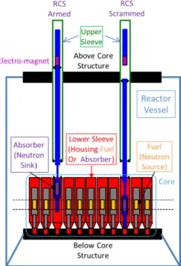
This topic applies to a large variety of reactor types: Pressurized Water Reactors (PWR) [1, 2], Boiling Water Reactors (BWR) [3] and Sodium-cooled Fast Reactors (SFR) [4, 5, 6, 7]. As illustrated in Figure 1, RCS designs, such as the CSR and the RBC systems, respectively described in [8] and [7], both instances for SFR-type reactors, are typically composed of:
• A Mobile Part (MP), which embeds the neutron absorbing material, retracted above the fissile core during reactor operation, and inserted into it during shutdown phases.
• Two static sleeves, which guide the MP during the insertion phase triggered by the reactor scram. The sleeves are respectively suspended underneath the Above Core Structure (ACS), for the Upper
Sleeve (US), and supported by the Below Core Structure (BCS), for the Lower Sleeve (LS), which is surrounded by neighboring fuel assemblies forming a densely packed lattice.
Figure 1: Example RCS Components Under seismic situations:
• The collective movements of the core assemblies, induced by the horizontal BCS excitation, lead to bending deformations of the LS. Because of the important stiffness provided by the close packing of core assemblies, the LS deformation constitutes a rigid boundary condition for the lower part of the MP.
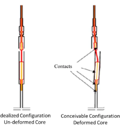
• The US also undergoes bending deformations, induced by the horizontal ACS excitation, albeit of lesser amplitude. These deformations constitute a semi-rigid boundary condition for the upper part of the MP, due to the finite stiffness of the US and absence of close packed structures surrounding it. As illustrated in Figure 2, the resulting misalignment between the LS and the US can generate multiple contacts with the MP, implying horizontal reaction forces that could be detrimental in two ways:
• Friction forces, resulting from these contacts, could counter-balance the gravitational force that drives the passive insertion of the MP into the reactor core, and thus delay reactor shutdown.
• Bending deformations and contact pressure, could induce various damages, such as excessive stress, relative to accepted design limits, and premature wear of the coated guide levels, where contacts are nominally expected to occur.
The French Atomic & Alternative Energy Commission (CEA) recently started a multi-year program to de-velop a set of simulation tools, and the associated experimental qualification tests, dedicated to RCS insertion reliability assessment. This work plan was initiated with a static tool, referred to as RC3, developed with the Cast3M Finite Element solver [9]. It is presently continued with the ongoing development and validation of a set of tools, based on analytic formulations and implemented with the Python programming language, within a toolbox called the Python Implementation for Reliability Assessment Tools (PIRAT) to cover:
Figure 2: Possible Contacting Surfaces
• Static studies: the Static Bresse Implementation tool (StaBI) is a finalized substitute for a finite element analysis, based on the Bresse formulation [10], designed for computing reaction forces (and resulting deformations, contact pressures, etc) induced by static displacements imposed by the sleeves.
• Dynamic studies: the Dynamic Euler-Bernoulli Implementation for Seismic Events tool (DEBSE), whose development is in progress, solves the dynamic Euler-Bernoulli equation, designed for produc-ing outputs similar to those of StaBI, but takproduc-ing into account their time evolution under some dynamic excitation relevant to seismic situations.
• Kinetic studies: the Step-by-step Insertion Kinetic Implementation tool (SIKI) will be developed to perform an iterative computation of the MP insertion, by relying on friction forces evaluated by means of the static/dynamic tool for each time step of the shutdown sequence, starting from scram, and until full insertion, including the final damping phase.
This paper discusses the progress and validation of the first two studies.
2
PIRAT
PIRAT uses Python as the script interpreter. Possible future development of the analysis performed by PIRAT, currently in discussion, could be to develop within the Cast3M framework. The current use of PIRAT is for an exploratory analysis that was only previouslly performed in [7] with issues that created a desire for analytical robustness. This desire was to allow a more flexible implementation for various geometries and desired outputs. The modular structure offered by PIRAT, in addition to the simple interface for numerical tools, are well adapted to the exploratory work considered. Within PIRAT, the full static solver and the preliminary work on the dynamic solver are presented in this section. Results from both of these solvers are compared against similar computations made with custom implementations of Cast3M to verify the accuracy, pending future comparison to experimental testing.
One of the unique characteristics of PIRAT, thanks to the Python implementation, is the ability to easily create new geometries and material properties. Geometry is inputted into PIRAT using an Excel spreadsheet containing the geometric properties and a material flag to be matched to user-defined properties. Adjusting the geometry, for example increasing the diameter of a section, is a simple change in the spreadsheet. With RC3, any geometric changes require a new model to be generated, meshed, and then analyzed. This is more time consuming since the intended use of PIRAT is for the initial design phases. During this phase, the geometry can vary over many iterations that can accumulate to a large amount of time for remodeling.
2.1 StaBI
For the first solver, a 1-to-1 replacement for RC3 is envisioned. The mathematics used in the StaBI solver are based on the Bresse formulations as presented in [10] and summarized as:
θ(z) = θ(z0) + ∫ z z0 Mf y(ζ) E(ζ)IGy(ζ)· dζ (1) ν(z) = ν(z0) + θ(z0)· (z − z0) + ∫ z z0 Mf y(ζ) E(ζ)IGy(ζ)· (z − ζ) · dζ, (2) where θ(x) is the angular displacement, ν(x) is the transverse displacement, Mf y(x) is the effective moment,
E(x) is the Young’s modulus, and IGy(x) is the area moment of inertia at location x. Since the system of
interest is a combination of multiple sections, the analysis is split into sections with both the transverse and angular displacement being continuous across each transition.
One of the major desired outputs of StaBI is the contact force values and locations between the MP and the sleeves (LS and US). Due to this, the effective bending moment is not known a priori. In order to calculate the force values, the superposition principle is used. At each location of possible contact, the response of the beam is computed for a unitary force. These responses are then collected into a matrix and used to solve for the forces via
Fk = [ ¯V (zk)]−1· [∆(zk)], (3)
with [∆(zk)] being the collection of displacements caused by the sleeves and [ ¯V (zk)] is the collection of
responses at each contact location due to a unitary force at each contact zk. Then these forces are used
to determine the final deflection of the MP and can be post-processed in order to get relevant data such as friction magnitude and bending stress in the beam.
The current implementation of StaBI has several assumptions; some are based on the Bresse theory and other are based solely on current implementations. The first assumption is that the beam is cantilevered at one end. Due to previous testing using RC3, this assumption is not expected to have a large effect on the results as compared to being pinned at the end. Past RC3 computations indicate that there is no large effect on the force locations and magnitudes due to the boundary condition at the top of the MP. Secondly, the force due to contact is assumed to be a point force that does not cause any surface deformation. This is to allow a simple determination of the applied forces due to the contact. Another implementation assumption is that for each section in the model is treated as a homogeneous and uniform cylinder. This creates the opportunity to avoid numerical integration; For a single point force, the effective moment within the beam can be known and then integrated analytically. The simplification comes in Equations 1 and 2 where the integrals are determined external to Python and the resultant is programmed in, reducing computational time and complexity in the program. There is a version of StaBI that utilizes numerical integration. However, there is a very large increase in computational time for the systems tested. For example, one evaluation using specific parameters using the analytical integration would take StaBI approximately one minute, and the same parameters but using a numerical integrator that is built into Python takes approximately 17 minutes on a fairly standard desktop computer. If only a single analysis is performed, this is still acceptable, but this might be constraining if StaBI is used for a kinetic evaluation that assumes quasi-static state at each time step via SIKI.
The last major assumption, which creates the most challenge, is how StaBI detects contact. This is done differently from the method used in RC3, which assigns a constraint on the stiffness matrix in order to account for contact. StaBI is a solver that does not require a mesh in order to determine the deflection of the MP, which RC3 requires. However, in order to determine if there is contact, a conforming mesh is assigned to all parts of the system. The current algorithm sweeps through that mesh and determines if the outer radius of the MP is in contact or past contact with the inner radius of the sleeves. Then StaBI assigns the point with the largest discrepancy as another contact point, and the algorithm is looped until there are no additional contact points. One major caveat found during testing is that enforcing a displacement very close to the actual sleeve
location will result in the algorithm detecting contact very close to previously determined locations, since each force is treated as a point force. This creates force values that are very large and nonphysical. In order to alleviate this issue, a clearance adjustment factor is used. This makes it such that there is a very small gap between the MP and the sleeve. Doing this generally produces larger force values, but allows for a more robust analysis. For the majority of the work performed in this paper, an adjustment factor of 80% of the clearance is applied. This is selected as an all-around value for the systems tested to produce reasonable results with no numerically determined parasitic contact.
2.1.1 Pseudo-code
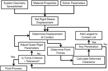
While there are many detailed steps in StaBI, the general work flow is broken-up into four major parts: 1) Setup and Geometry, 2) Quasi-Rigid Convergence, 3) Contact Determination, and 4) Post-Processing. These are the steps currently implemented into the static solver and are similar steps to those that are expected to be implemented into the dynamic solver as well. Step 1 is specific to each system tested. This includes: generating the geometry, setting material properties, determining convergence criteria, setting the sleeve locations, and determining the step size for the contact determination. These all are different depending on the system being investigated and what the user desires. Step 2 is a large loop that contains step 3 within it. If a subsystem (US for example) is determined to be quasi-rigid, then iterations on the displacement of that subsystem must be performed to create a quasi-static equilibrium state of the system. Currently, this is done by comparing the calculated force value on the MP and the force value on the quasi-rigid subsystem at the same location. Step 3 loops through adding contact locations until there is no additional contacts found. Once step 2 is converged, then the post-processing of the data can occur in step 4. This would output values such as: bending stress, total friction in the system, and Hertzian contact pressure. A more detailed step flow chart is presented in Figure 3.
Figure 3: Flow Chart of StaBI for Guided Systems with Both Rigid and Quasi-Rigid Sleeves
2.2 Preliminary DEBSE
One of the main goals of the PIRAT tool is to perform the analysis in the dynamic domain to ensure the insertion reliability during a seismic event. Initially, the expansion of PIRAT to handle dynamic situations is to replace the Bresse’s equations of motion with the dynamic Euler-Bernoulli beam equations of motion. This increases the dimension of the system by introducing a dependency of time. Current use of one dimension in space is a simplification for the current work that can be expanded in the future to account for any drop velocity. The governing differential equation of motion becomes:
∂2 ∂x2(EI(x) ∂2w(x, t) ∂x2 ) + ρA(x) ∂2w(x, t) ∂t2 = q(x, t), (4)
where w(x, t) is the transverse displacement of the beam, EI(x) is the structural rigidity, ρA(x) is the linear mass density, and q(x, t) is the externally applied distributed load. One thing to note is that this formulation does not account for axial stretching. As will be discussed in the comparison of DEBSE to Cast3M, this stretching might be an important factor for select modes. For the majority of the analysis in this paper, it is assumed that all driving loads are either internal to the system or are applied as a time-dependent boundary conditions. The implementation of these boundary conditions are similar to the method used in [11]. Simply, the displacement of the beam is a combination of the free-vibration and the time-dependent boundary conditions. One example of how this can be written is:
w(x, t) = ϕ0(t)δ(x) + ϕL(t)δ(x− L) + u(x, t) (5)
where ϕx(t) is the time dependent boundary condition at x, δ(x) is the Dirac delta function, and u(x, t) is
the free-vibration of the beam subject to elementary boundary conditions such as: pinned, clamped, and free. With the knowledge that future work will include free-vibration, the preliminary dynamic analysis is a veri-fication of the dynamic properties of the example system, in particular the MP subsystem. The free-vibration analysis being used in DEBSE is currently based on modal decomposition. This allows for a separation of time and space in the governing equations of motion and can be written as:
u(x, t) =∑
n
ψn(x)qn(t), (6)
where ψn(x) are the deflection shapes, also called mode shapes, and qn(t) is the time dependent contribution
of mode n [11]. While this summation is countably infinite, it is typically truncated based on frequency via the natural frequencies. Using this modal decomposition allows for the partial differential equation in Equation 4 to become a summation of independent ordinary differential equations.
This system of interest contains some interesting aspects that require some special considerations. The major interesting aspect is the geometric discontinuities across different sections of the MP. Each section of the MP is modeled as a homogeneous, uniform cylinder with the difference between sections occur instantaneously, providing no derivative at that point of the beam. The cylinder model is a current simplification to allow for a more simple evaluation. There are analytical representations of mode shapes for functionally variant cross-sections [12, 13, 14] that will be included as this tool is further developed. This is mainly an issue with the first term in Equation 4 that looks at how the structural rigidity changes along the beam. In order to account for this step change, each section is thought up as a homogeneous beam with specified boundary conditions, similarly to the method used in [15]. The external boundary conditions are still enforced, but at the internal boundaries, mode shape continuity is enforced. This can be expressed as:
ψn,i(Li) = ψn,i+1(0) (7a)
∂ψn,i ∂x (Li) = ∂ψn,i+1 ∂x (0) (7b) EIi ∂2ψn,i ∂x2 (Li) = EIi+1 ∂2ψn,i+1 ∂x2 (0) (7c) EIi ∂3ψn,i ∂x3 (Li) = EIi+1 ∂3ψn,i+1 ∂x3 (0), (7d)
with Li being the length and ψn,ibeing the mode shape of section i for mode n. Using this formulation, it
is assumed that each section has a local coordinate system and the modal deflection at any location can be determined by:
ψn(x) = ψn,i(x− x0i) if x∈ [x0i, xf i], (8)
where x0iis the starting location and xf iis the ending location of section i in the global coordinate system.
For the validation of DEBSE, Cast3M is used to provide natural frequencies and mode shapes for the MP system. These are chosen in order to test the basic uses for the dynamic solver. Both natural frequencies and mode shapes are not dependent on user-input. Other dynamic data, such as frequency response functions and time history, require the analyst to decide some damping factor and time-dependent boundary conditions in order to evaluate. Since this can be chosen to be the same for Cast3M and DEBSE, any differences found in these two are primarily due to the differences in the mode shapes and frequencies.
Applying the modal decomposition to Equation 4, the space component of this equation becomes: ∂4ψn,i(x)
∂x4 = β 4
n,iψn,i(x), (9)
where βn,iis an unknown coefficient that is related to the natural frequency of the mode n and the material
properties of section i. The general solution to this differential condition is:
ψn,i(x) = a1,n,isin(βn,ix) + a2,n,isinh(βn,ix) + a3,n,icos(βn,ix) + a4,n,icosh(βn,ix), (10)
with ak,n,ibeing unknown coefficients for the mode shapes. These coefficients are determined based on the
constraints of the system, which can be written as: Ex0 D0 G .. . an,i .. . = [0] (11) or [B][an] = [0], (12)
where Ex is the external boundary condition for x = 0 and D is the external boundary condition at x = L applied to the mode shapes, G is the continuity conditions given in Equation 7, and anare the collection of
mode shape coefficients with an,i= [a1,n,i, a2,n,i, a3,n,i, a4,n,i]T.
The constraint matrix [B] is a function of the coefficient β that is a function of frequency. When the frequency is set to a natural frequency, the constraint matrix is rank deficient, meaning that the determinate is equal to zero [16]. In order to determine the natural frequency in DEBSE, a Newton-Raphson method is used on the determinate of the constraint matrix. For the initial points of the Newton-Raphson method, the natural frequency of a uniform beam containing the mean properties of the MP subject to the external boundary conditions is used. Since a uniform beam with elementary boundary conditions contains a known analytical solution, that value is used. This makes the assumption that this mean natural frequency is relatively close to the true natural frequency. In order to ensure this, a redundancy check is performed on the natural frequencies to ensure that the same mode is not considered multiple times. Additionally, the natural frequencies found in Cast3M are also inputted as initial points to determine the natural frequencies before the redundancy check. It was found during testing, that using an uniform beam with average material properties would occasionally skip a mode of vibration. Alternate initial starting points for the Newton-Raphson method are being investigated, such as an interactive input showing the frequency response function to ensure that each peak is selected and evaluated. The mode shapes are determined at each natural frequency by setting one component to a specified value since the constraint matrix is rank deficient.
Once these are determined in DEBSE, they can be compared to the results from Cast3M. The error on the natural frequencies is calculated by a percent difference once the desired mode in the model is selected. In
order to select which DEBSE mode corresponds to the Cast3M mode, a comparison between the mode shapes is required. For this analysis, the modal assurance criterion (MAC) is used. The MAC can be determined by:
M ACij =
(ψTi ψj)2
(ψTi ψi)(ψjTψj)
, (13)
where i and j are mode numbers. The MAC calculation is performed for each mode generated by DEBSE and by Cast3M. This MAC value has a range of [0, 1] with a MAC value of 0 implying that there is no correlation between the modes and a value of 1 implying that there is a perfect correlation between the modes. An important note to make is that the MAC values do not prove orthogonality, they just imply correlation. This is similar to the saying “Correlation does not ensure dependency” from the statistics field. Using a method like this will allow a quantitative proof of the corresponding mode shapes. This is used to filter out motion that is not described by a method, in this report the axially coupled modes of Cast3M, and show if there is any issue with the convergence of the Newton-Raphson approach to determine the natural frequencies.
3
Example System
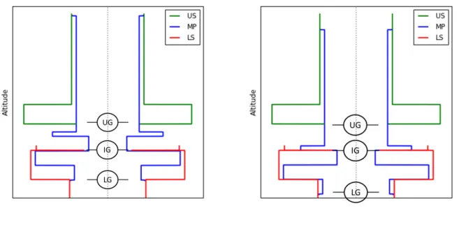
In order to test PIRAT, a simplified but realistic RCS system is used. The requirement for the type of system is a beam like object that is guided by sleeves, such as the one pictured in Figure 4. This is taken as a similar system to the one analyized in [5, 6, 7]. There are some differences in these systems and the dimensions are not given. An estimation of the length of the beam and comparative dimensions was performed, resulting in the example system used in this work. In order to represent the sleeves, a polynomial is used for the LS and the US is treated as quasi-rigid. Some features, such as the dash-pot, are removed for simplification since previous testing showed no significant changes due to these additional complexities.
(a) Zero Stroke (b) Full Stroke
Figure 4: Geometric Configuration of the Example System
This system has a maximum stroke around 1000mm, meaning that the MP can move vertically by that amount. To test this range, stroke values from 0 to 1000mm in increments of 10% the maximum stroke are simulated using StaBI. There are three main points of reference that correspond to expected guide regions shown in Figure 4. The first is the bottom section of the MP, thus causing the contact location to vary in
the global coordinate system. If the global reference frame is considered, the Lower Guide (LG) produces a moving contact, which could add some difficulties to the dynamic analysis if the MP is allowed to drop. The second area is the guide region at the top of the LS, call the Intermediate Guide (IG). This area has a larger clearance compared to the other guide regions, but is expected to produce the largest contact force due to the large imposed displacements. The final expected contact location is the Upper Guide (UG). This is located at the bottom of the US and has the smallest clearance. The UG is also the location used for the quasi-rigid convergence loop.
4
Static Misalignment
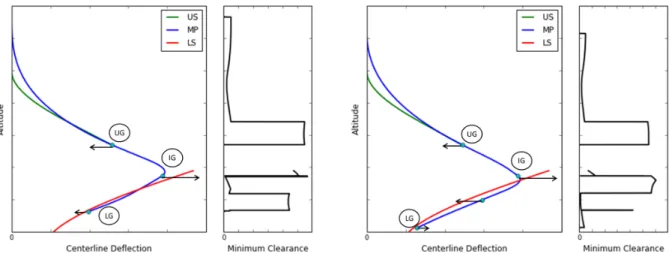
For this static solver, both StaBI and RC3 produced the same contact points for stroke values up to 800mm. In the cases with stroke values greater than 800mm, StaBI detected a parasitic contact between the LG and the IG. The first result to report is the deformation shape of the MP in Figure 5a. This figure shows the center-line deflection of the three subsystems, contact locations (as cyan dots), and the minimum clearance of the MP at each altitude point for the case of a stroke value of 0mm. This shows that there is contact at each of the guide areas that contain a reduced clearance resulting in a total of three nominal contacts. One interesting aspect of Figure 5a is the near parasitic contact within the US. Figure 5b shows the same data for when there is a full stroke. Some interesting things to note are the parasitic contact between the LG and IG and the change in sign for the contact force of the LG.
(a) Zero Stroke (b) Full Stroke
Figure 5: Example Deformation Shape of Example System with Vectors Representing Relative Force Mag-nitude and Direction
These deflections are compared to the results from RC3 using the same displacement for the quasi-rigid US, which is scaled to the displacement at the UG, and can be seen in Figure 6a. In Figure 6, the values for the detected contacts are also presented. These include both using a tolerance adjustment factor of 80% and 90% to show the increase in accuracy. One thing to note, the RC3 simulations are re-performed for each adjustment factor. This is due to each case having a slightly different US profile due to the deflection at the UG.
There is some small differences between RC3 and StaBI shown in Figure 6a. First, for the areas that are bounded by the sleeves, StaBI reports less deflection than RC3 and the opposite of that when the MP is not bounded by the sleeves (between the IG and UG). Besides that small shift, there is a noticeable discrepancy near the LG. The cause of this is unknown, since there is a tight tolerance at the LG level. One possibility is the discrepancy between StaBI and RC3 on the force magnitude. For the LG on this particular example, StaBI
(a) Stroke Value of 0 mm (b) Stroke Value of 700 mm
Figure 6: Comparison of Deflected Shape of Example System
detected a force of 240N while RC3 detected a force of 220N . This is one of the largest differences found between the two methods but is still within 10%. Another possibility is based on the contact algorithm. The contact algorithm used in RC3 sweeps through the mesh on the sleeves and finds the closest mesh point of the MP within tolerance. There is a possibility that for this stroke value, the algorithm did not evaluate a mesh point on the LG, but only to another section of the MP. One thing to note is that for a stroke value of 0mm, StaBI and RC3 has the worst agreement among the cases where the same contact zones are determined. To show a closer agreement, a stroke value of 700mm is shown in Figure 6b. This shows that there is almost no difference between StaBI and RC3 except a very small shift that was also noted in Figure 6a, but with a smaller magnitude of difference.
Qualitatively, the benchmark between StaBI and RC3 produces satisfactory results. By looking at the per-centage difference between the magnitude of the contact forces, a similar conclusion can be determined. For the cases where StaBI and RC3 produced the same contact zones, there was an average percent difference of 5.6% with a maximum difference of 9.9%. This level of accuracy is sufficient to say that when the contact algorithms detect the same locations, either StaBI or RC3 will give a good result.
It is an important note that these results used a tolerance adjustment factor of 0.80, meaning that 80% of the clearance is enforced for the contacts. If this factor is increased to 90%, the accuracy increases. For this system, the average percent difference is 1.5% with a maximum of 5.0% in magnitude. One interesting effect of this increase is that the forces from StaBI are not always higher in magnitude compared to RC3. This shows that there is not a guaranteed conservative estimate on the contact forces as originally thought. When the adjustment factor is increased to 95%, StaBI detects parasitic contact within the same zones as other previously determined contact locations. In particular, StaBI usually detects a second contact at the LG causing the forces at the LG to increase substantially, on the order of 100N to 20, 000N . There is still future work in the determination of the tolerance adjustment factor and the contact algorithm in general. This can only be done with either a known benchmark (simplified system tested by various methods) or some experimental validation.
5
Preliminary Dynamic Analysis
In order to test the accuracy of the DEBSE solver, six different configurations are tested for the MP using a combination of free (F), clamped (C), and pinned (P) boundary conditions applied to the top of the MP and
the LG. These same configurations were also used in Cast3M in order to verify the natural frequencies and mode shapes. The algorithm used in Cast3M for modal analysis requires one of two inputs, a set number of modes or a range of frequencies. For this comparison, the frequencies of interest are those less than 100Hz. This was chosen since the seismic frequencies are expected to be in the low range. The MP has between 10 and 13 elastic natural frequencies within this range depending on the boundary conditions.
The first results for validation purposes is the comparison of mode shapes. This is done by applying the MAC formula in Equation 13 to the modes generated by DEBSE and the modes generated by Cast3M. The results from these calculations can be seen in Figure 7 for the six combinations of boundary conditions. As a note of nomenclature, the first word in the sub-caption refers to the boundary condition at the bottom of the MP, the LG, and the second word refers to the condition at the top. For the majority of the modes, there is an almost one-to-one relationship between the DEBSE modes and the Cast3M modes. In a typical analysis, a MAC value greater than 0.90 would be considered the same mode.
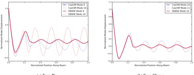
For the majority of the modes, the MAC value is around 0.99 for the corresponding mode and values less than 0.10 for the non-corresponding modes with the exception of the Free-Pin and Free-Clamped boundary conditions. In the Free-Pin configuration, there is no Cast3M mode for the tenth elastic mode discovered in DEBSE. Additionally, the tenth mode in Cast3M is very similar to the ninth mode from DEBSE producing a MAC value of 0.63. These four modes are shown in Figure 8a with the blue curves being from Cast3M and the red curves being from DEBSE. The first thing to note is that Mode 9 for both Cast3M and DEBSE overlap nearly perfectly and are indistinguishable from each other on this plot. Mode 10 for each produce similar shapes, but with a phase shift and different amplitudes. The true cause of this is unknown, but it is expected to be due to in part by the stepped-beam properties. With drastic changes in the geometry and material properties, there is a possibility of local stretching that is characterized in Cast3M that is undetectable by DEBSE in the current implementation. DEBSE uses the small deformation version of the Euler-Bernoulli beam equation. Alternate formulations are possible that can account for axial stretching, but it not currently implemented. Further investigation is being performed to determine the exact cause of this discrepancy. A similar case can be seen for the Free-Clamped boundary conditions. For this, there is no missing DEBSE mode, but there is a strong coupling between Cast3M mode 10 and 11. The MAC value for DEBSE mode 10 and Cast3M mode 11 is 0.835. This is a very large MAC value for separate modes. To further investigate, these modes shapes are plotted in Figure 8b. Cast3M and DEBSE mode 10 are almost identical with mode 11 from Cast3M matching the curve but with different amplitudes further along the beam. The cause of this is also unknown, but might be due to the local stretching that was previously discussed for the Free-Pin boundary condition.
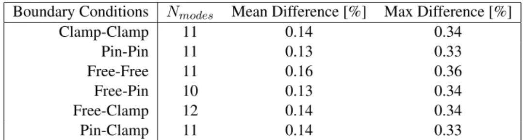
The other main validation is the difference in natural frequencies between the two methods. This is computed as a percentage difference of the corresponding modes that contained MAC values larger than 0.90. The results from this comparison can be seen in Table 1. For the modes that matched well, there is very good agreement in the natural frequencies, resulting in a maximum percent difference of 0.36%. This shows that for a given bending mode, DEBSE is able to correctly identify the natural frequency and mode shape.
Boundary Conditions Nmodes Mean Difference [%] Max Difference [%]
Clamp-Clamp 11 0.14 0.34 Pin-Pin 11 0.13 0.33 Free-Free 11 0.16 0.36 Free-Pin 10 0.13 0.34 Free-Clamp 12 0.14 0.34 Pin-Clamp 11 0.14 0.33
1 2 3 4 5 6 7 8 9 10 11 Cast3M Modes 1 2 3 4 5 6 7 8 9 10 11 D EBS E M od es MAC 0.1 0.2 0.3 0.4 0.5 0.6 0.7 0.8 0.9 (a) Pin-Pin 1 2 3 4 5 6 7 8 9 10 11 Cast3M Modes 1 2 3 4 5 6 7 8 9 10 11 D EBS E M od es MAC 0.1 0.2 0.3 0.4 0.5 0.6 0.7 0.8 0.9 (b) Free-Free 1 2 3 4 5 6 7 8 9 10 11 Cast3M Modes 1 2 3 4 5 6 7 8 9 10 11 D EBS E M od es MAC 0.1 0.2 0.3 0.4 0.5 0.6 0.7 0.8 0.9 1.0 (c) Clamp-Clamp 1 2 3 4 5 6 7 8 9 10 11 Cast3M Modes 1 2 3 4 5 6 7 8 9 10 11 D EBS E M od es MAC 0.1 0.2 0.3 0.4 0.5 0.6 0.7 0.8 0.9 (d) Free-Pin 1 2 3 4 5 6 7 8 9 10 11 12 13 Cast3M Modes 1 2 3 4 5 6 7 8 9 10 11 12 D EBS E M od es MAC 0.1 0.2 0.3 0.4 0.5 0.6 0.7 0.8 0.9 (e) Free-Clamp 1 2 3 4 5 6 7 8 9 10 11 Cast3M Modes 1 2 3 4 5 6 7 8 9 10 11 D EBS E M od es MAC 0.1 0.2 0.3 0.4 0.5 0.6 0.7 0.8 0.9 1.0 (f) Pin-Clamp
0.0 0.2 0.4 0.6 0.8 1.0
Normalized Position Along Beam
−0.5 0.0 0.5 1.0 No rm ali ze d M od al Disp lac em en t Cast3M Mode 9 Cast3M Mode 10 DEBSE Mode 9 DEBSE Mode 10 (a) Free-Pin 0.0 0.2 0.4 0.6 0.8 1.0
Normalized Position Along Beam
−0.4 −0.2 0.0 0.2 0.4 0.6 0.8 1.0 1.2 No rm ali ze d M od al Disp lac em en t Cast3M Mode 10 Cast3M Mode 11 DEBSE Mode 10 (b) Free-Clamp
Figure 8: Normalized Mode Shapes for Select Boundary Conditions
6
Remarks/Future Work
The static solver, StaBI, is shown to produce similar results to RC3 when the contact algorithms produce the same contact locations. This is the major part of the future work for this solver. The contact algorithm of adding an additional contact for each iteration with no ability to remove a contact is the portion of the solver that requires the most investigation. It is currently unknown how this algorithm will be changed, but it is difficult to determine which algorithm is a better match to the real system without any experimental data to compare to. Gathering of this experimental data is currently being discussed and planned. This data is expected to be gathered at either the CARNAC facility in Cadarache [17] or at the TAMARIS facility in Saclay [18].
The next step for using the static solver would be to introduce the SIKI tool using the StaBI solver. This system is expected to drop in case of a seismic event. So in order to get some information about this insertion, a kinetic analysis is expected to be performed. This entails using an explicit ”time-marching” algorithm with each time step being treated as quasi-static. The analysis would not require much changes to the solver, but might require some optimization in order to allow for performing the analysis within a reasonable time. While the natural frequencies and mode shapes are not the desired end result for the dynamic expansion, they do provide a useful foundation to show that the solver can handle the simple calculations. There is a possible issue when it comes to computational time for each simulation. Since the natural frequencies are determined by taking the determinate of the constraint matrix, as the matrix increases in size, the required time to determine each natural frequency increase. This matrix increases in size as more sections are introduced since there are four additional coefficients and four continuity equations that are added to the system. While this is not an issue for just looking at the MP, this might become more of an issue when contact is added. One possible method to introduce contact is to replace the location of contact with a moving Pin boundary condition. Using this method, along with modal decomposition, would require an initial determination of frequencies and an additional determination for each addition and removal of contact locations. Currently for the MP, it takes roughly ten minutes to compute the first fifteen natural frequencies while checking for duplicates. It also takes approximately ten minutes to calculate the mode shapes for the MP with 1206 node points. One expected future work is to better optimize these procedures or find an alternative approach to determine the time history of the system. A possible alternative would be to apply the contact as constraints on the system. This would allow for a single modal characteristics evaluation and provides extra equations that might allow for the determination of the contact force required.
func-tion of time. This includes: contact determinafunc-tion, force calculafunc-tion at contact locafunc-tions, contact removal, modeling contact, and moving contact. One interesting aspect about performing this dynamic analysis is that this type of analysis has not previously been performed at CEA. Previous iterations used a quasi-static approach to simulations and then used experimental systems to ensure dynamic capabilities for qualification. Using this dynamic simulations will be able to replicate the dynamic experiments at a fraction of the cost, and allow for additional information to be determined providing more information to the design engineers. While a dynamic experiment will still be required for qualification, there is less chance of geometric changes due to failure resulting in requiring additional experimentation with a new geometry. Using this PIRAT tool will allow for engineers to produce a safer system at an expectantly lower cost.
7
Conclusions
PIRAT is a novel tool that allows the calculation of contact location and forces using an analytical approach. The static solver uses the Bresse’s formulations that allow for the determination of the displacement of a system due to a force and also allows for an inverse solution in order to determine the force magnitudes due to constrained displacements. This tool is used on an example prototype system and is compared to previous work done using finite elements in Cast3M called RC3. These two methods show very good agreement for the majority of cases. This agreement did not occur when the different contact algorithms produced different contact locations. Without experimental validation data, it is unsure of which algorithm is more realistic to the physical system, thus experimental testing is currently being planned.
The final desire for this PIRAT tool is to perform the same analysis in a dynamic sense. While this is a complicated expansion, some preliminary work has been performed for the dynamic solver. This work is comprised of a modal analysis of the Mobile Part with no contact with the Lower or Upper Sleeve. The results presented are the natural frequencies and the mode shapes of the step-changed Mobile Part beam. These results are compared to a similar analysis performed in Cast3M using the built-in eigen solvers. This compares the shape and natural frequencies for the modes less than 100Hz. DEBSE was able to produce nearly identical results for the natural frequencies and mode shapes except when there was possibly axially stretched modes found in Cast3M, which uses 2D finite elements compared to 1D equations of motion for DEBSE. For modes that had a MAC value larger than 0.90, the difference in the natural frequency was less than 0.4%.
This StaBI tool has proven to be accurate for the static analysis compared to the work previously performed using finite elements in a custom implementation in Cast3M. While there are differences in the contact algo-rithms, these tools provide very similar results for most cases tested. The differences between the algorithms and the physical system are not yet known, but are in planning. Since the desire of analysis is to predict if there is a failure during a seismic event, preliminary steps are performed in creating a dynamic solver within PIRAT. Initially, this work compares the natural frequencies and mode shapes of DEBSE and those produced by finite elements in Cast3M. DEBSE shows to be extremely accurate while being much easier to make design changes compared to Cast3M due to the implementation. The PIRAT tool is able to take beam-like structures that are bounded by guiding sleeves and determine the contact force and deflection caused primarily by the seismic induced misalignment.
References
[1] K. Fujita, Y. Shinohara, K. Nanbu, T. Nakatogawa, and T. Nomura. Scram characteristics of control rods of pressurized water reactor under seismic conditions. JSME international journal, 30(267):1450– 1457, 1987.
[2] B Collard. Rod cluster control assembly drop kinetics with seismic excitation. In Proceedings of the 11th international conference on nuclear engineering ICONE 11, Tokyo, Japan, April 2003. ICONE-36419.
[3] Y Watanabe and Y Motora. Analysis of cr scrammability characteristics on the condition of the forced vibration of fuel assemblies. In Transactions of the 7. international conference on structural mechanics in reactor technology. Vol. F, 1983.
[4] A. Morrone, A.N. Nahavandi, and W.G. Brussalis. Scram and nonlinear reactor system seismic analysis for a liquid metal fast reactor. Nuclear Engineering and Design, 38(3):555 – 566, 1976.
[5] D. Brochard and P. Buland. Seismic qualification of SPX1 shutdown systems - tests and calculations. In Proceedings of the ICONE-11 Conference, Bologna, Italy, October 1987.
[6] M.N. Sundaran, R. Vijayashree, S. Raghupathy, and P. Puthiyavinayagam. Experimental seismic quali-fication of diverse safety rod and its drive mechanism of prototype fast breeder reactor. In Proceedings of the FR17 Conference, Yekaterinburg, Russia.
[7] M. Zabi´ego, D. Lorenzo, T. Helfer, and E. Guillemin. Insertion reliability studies for the RBC-type control rods in ASTRID. In Proceedings of FR17 Conference, Yekaterinburg, Russia, June 2017. Paper IAEA-NC-254-120.
[8] V. R. Babu, R. Veerasamy, S. Patri, S. I. S. Raj, S.C.S.P. K. Krovvidi, S.K. Dash, C. Meikandamurthy, K.K. Rajan, P. Puthiyavinayagam, P. Chellapandi, et al. Testing and qualification of control & safety rod and its drive mechanism of fast breeder reactor. Nuclear Engineering and Design, 240(7):1728–1738, 2010.
[9] CAST3M. Cast3M is a research fem environment; its development is sponsored by the French Atomic and Alternative Energy Commission. http://www-cast3m.cea.fr.
[10] J. Courbon. Th´eorie des poutres. Techniques de l’ing´enieur, (C2010), 1980. (In French).
[11] P. F. Gou and K. K. Panahi. Analytical solution for beam with time-dependent boundary conditions versus response spectrum. In Proceedings of the 9thInternational Conference on Nuclear Engineering, Nice, France, April 2001.
[12] S. Y. Lee and S. M. Lin. Dynamic analysis of nonuniform beams with time-dependent elastic boundary conditions. Journal of applied mechanics, 63(2):474–478, 1996.
[13] D. W. Chen and J. S. Wu. The exact solutions for the natural frequencies and mode shapes of non-uniform beams with multiple spring–mass systems. Journal of Sound and Vibration, 255(2):299–322, 2002.
[14] Y. Huang and X. F. Li. A new approach for free vibration of axially functionally graded beams with non-uniform cross-section. Journal of sound and vibration, 329(11):2291–2303, 2010.
[15] M. A. Koplow, A. Bhattacharyya, and B. P. Mann. Closed form solutions for the dynamic response of Euler–Bernoulli beams with step changes in cross section. Journal of Sound and Vibration, 295(1-2):214–225, 2006.
[16] M. Avcar. Free vibration analysis of beams considering different geometric characteristics and bound-ary conditions. International Journal of Mechanics and Applications, 4(3):94–100, 2014.
[17] T. Catterou, V. Blanc, G. Ricciardi, S. Bourgeois, and B. Cochelin. Numerical strategy for dynamic simulations of impacts on SFR fuel pins and experimental validation. Journal of Nuclear Engineering and Design. In Submission.