HAL Id: halshs-00155709
https://halshs.archives-ouvertes.fr/halshs-00155709
Submitted on 19 Jun 2007HAL is a multi-disciplinary open access
archive for the deposit and dissemination of sci-entific research documents, whether they are pub-lished or not. The documents may come from teaching and research institutions in France or abroad, or from public or private research centers.
L’archive ouverte pluridisciplinaire HAL, est destinée au dépôt et à la diffusion de documents scientifiques de niveau recherche, publiés ou non, émanant des établissements d’enseignement et de recherche français ou étrangers, des laboratoires publics ou privés.
and Comparative Dynamics in Competitiive Markets
Gaël Giraud
To cite this version:
Gaël Giraud. The Limit-Price Dynamics - Uniqueness, Computability and Comparative Dynamics in Competitiive Markets. 2007. �halshs-00155709�
Centre d’Economie de la Sorbonne
Maison des Sciences Économiques, 106-112 boulevard de L'Hôpital, 75647 Paris Cedex 13
http://ces.univ-paris1.fr/cesdp/CES-docs.htm
ISSN : 1955-611X
The Limit-Price Dynamics — Uniqueness, Computability and Comparative Dynamics in Competitive Markets
Gaël GIRAUD 2007.20
Uniqueness, Computability, and Comparative Dynamics in
Competitive Markets
Ga¨el Giraud1), 2)∗
1) Paris School of economics, CNRS 2) Universit´e Paris-1 Panth´eon-Sorbonne
[email protected] April 30, 2007
Abstract.— In this paper, a continuous-time price-quantity trading process is defined for exchange economies with differentiable characteristics. The dynamics is based on boundedly rational agents exchanging limit-price orders to a central clearing house, which rations infinitesimal trades according to Mertens (2003) double auction. Existence of continuous trade and price curves holds under weak conditions, and in particular even if there is no long-run competitive equilibrium. Every such curve converges towards a Pareto point, and every Paretian allocation is a locally stable rest-point. Generically, given initial conditions, the trade and price curve is piecewise unique, smooth, and computable, hence enables to effec-tively perform comparative dynamics. Finally, in the 2 × 2 case, the vector field induced by the limit-price dynamics is real-analytic.
Keywords: Non-tˆatonnement, Price-quantity dynamics, Limit-price mechanism, My-opia, Computable General Equilibrium.
R´esum´e.— On d´efinit un processus d’´echanges en prix et en quantit´es et en temps continue, pour des ´economies diff´erentiables. La dynamique est fond´ee sur la rationalit´e limit´ee d’agents myopes qui adressent des ordres de prix-limites qu’ils adressent `a une agence de clearing centrale, laquelle rationne les ´echanges infinit´esimaux en fonction de l’ench`ere double de Mertens (2003). L’existence de courbes de prix et d’´echanges est v´erifi´ee sous de faibles conditions, en partic-ulier en l’absence d’´equilibre concurrentiel de long-terme. Toute courbe d’´echange converge vers un optimum de Pareto, et inversement tout optimum est un point stationnaire localement stable de la dynamique G´en´eriquement, `a conditions ini-tiales donn´ees, la courbe d’´echanges et de prix est unique par morceaux, lisse et calculable, ouvrant la possibilit´e d’une dynamique comparative effective. Enfin, dans le cas 2 × 2, le champ de vecteurs associ´e `a la dynamique est r´eel-analytique. Mots-Clefs: Non-tˆatonnement, dynamique en prix et en quantit´es, m´ecanisme de prix-limite, myopie, ´equilibre g´en´eral calculable.
JEL Classification. C02, C61, C62, C63, D46.
∗I wish to thank C´eline Rochon, Dimitrios Tsomocos, Prof. Jean-Marc Bonnisseau, Bernard Cornet and John Geanakoplos, as well as participants to seminars at Paris-1, Strasbourg-1, Bielefeld, Venice, Mumbay for useful comments. Errors are the sole responsability of the author.
1
Introduction
In this paper, we investigate a continuous-time price-quantity process for pure-exchange Arrow-Debreu economies with a continuum of traders and finitely many commodities. As such, this paper takes place within the litterature devoted to the “non-tˆatonnement” ap-proach1 Real trades are supposed to take place across time, so that, if we allow a passage of time, and several such, the initial endowment point becomes rapidly lost in the shuffle. Therefore, by contrast with price adjustment processes, the basic notion of steady state can no longer be provided, in general, by the concept of Walras equilibrium inherited from static General Equilibrium Theory (GET hereafter). Instead, it is replaced by that of price equi-librium, i.e., of a Pareto-efficient state sustained by some price equilibrium vector that turns it into a no-trade competitive equilibrium. As a consequence, since Pareto points are not locally unique, the uniqueness of trajectories becomes a crucial matter. And there, a new difficulty must be faced: Indeed, it is easy to show that, given fixed initial conditions, any continuous ordinary differential equation admits either a globally unique solution trajectory or infinitely many such solutions (see Appendix 6.1). In other words, the comfortable middle ground obtained within the static framework, where the set of static equilibria is shown to be generically finite, cannot have any counterpart in non-tˆatonnement dynamics. It is there-fore not a surprise if all the non-tˆatonnement processes we are aware of exhibit some kind of strong indeterminacy. To take but two examples, Schecter (1977) proved that, for every initial condition, every point in the contract curve is a rest-point of some solution to Smale’s (1976) price-adjustment process; a similar accessibility result was proven by Bottazzi (1994) for Champsaur & Cornet (1990)’s refinement of Smale’s process. In either case, one can make no prediction as to where on the optimal set a sequence of trades beginning at some initial endowment ω will end, except that it will end at a point that is (weakly) preferred to ω by every agent.
In this paper, we propose a variant of Smale’s (1976) and Champsaur & Cornet’s (1990) price-quantity adjustment processes that aims at solving the problems just outlined. Traders are boundedly rational, so that they do not aim to instantaneously maximize their long-run utility function (or the utility of their own clients if they are, say, middlemen acting for a clientele). Rather, they try to move their portfolio in the direction inducing the steepest increase of their (current) utility. To put our formalism yet another way: at every instant of time t, agents play in a (linear) marginal economy, where they exchange infinitesimally small amounts of commodities so as to maximize their short-term, marginal (linear) utility function. The economic rationale for such a myopic behavior is not new: On the one hand, it makes sense to assume that, on the very short-run, people behave as if they were risk-neutral. On the other hand, even chess International Grandmasters do not calculate more than four or five moves ahead, and it has been argued that, under quite reasonable circumstances, seeing further into the future does not mean seeing better.2 As for the micro-structure of
infinitesi-mal trades, it mimics that of financial markets: Traders anonymously send limit price orders to a central clearing house. Hence, they even need not know with whom they are trading. A rationing function — namely Mertens’ (2003) limit-price mechanism — instantaneously matches demand and supply. Once markets operated at time t, new bids and offers are made at t + dt, which automatically replace those just sent. The main results are as follows:
1) Existence of solution trajectories is guaranteed under fairly weak assumptions — in particular without strict monotonicity or boundary conditions on utilities, or else without any survival restriction on initial endowments. We exhibit examples where static Walras equilibria fail to exist, and yet our dynamics admits solution paths. Moreover, every solution path admits some price-equilibrium as cluster-point. Conversely, price equilibrium is locally stable3 for our dynamics. This leaves open the possibility that a solution trajectory circles
infinitely many times around a price equilibrium.
1See Hahn (1971), Jordan (1986) and Herings (1995) for early surveys. 2See, e.g., Gray & Geanakoplos (1991) and the literature therein.
3Local stability means that every solution curve that does not start too far away from a given rest point
2) Our non-tˆatonnement process works with myopic (but rational) traders who need only know the local shape of their indifference manifolds, and publicly observe prices at each point in time. On the other hand, at variance with, e.g., Kumar & Shubik (2002), the rules of the game to which consumers take part are independent from the characteristics of its players.
3) For a generic choice of utilities and initial endowments, we get the (global) uniqueness of the solution path to the corresponding Cauchy’s problem within a certain time interval [0, ε) (ε > 0). Moreover, the restriction to that time interval [0, ε) of every such solution path is smooth, and depends smoothly upon initial conditions. Put differently, the feasible set admits a partition into an open and dense subset of “regular” economies (for which the vector field of our dynamics is real-analytic) and a finite union of low-dimensional, smooth, critical submanifolds (with empty interior). When the trajectory of trades happens to cross non-transervally such a critical submanifold — and only under such exceptional circumstances — smoothness and/or uniqueness of the trade and price curve may fail. On the other hand, for every economy involving two households and two goods, the vector field associated to our dynamics is real-analytic on the whole interior of the feasible set.
4) Every trajectory can be effectively computed, which is a must for dynamic comparative purposes. We do not address this last issue in its full scope in the present paper, but content ourselves with fully characterizing all the portrait phases of our dynamics in the Edgeworth box of 2 × 2 economies. In particular, we show that the vector field is real-analytic. A companion article will offer the general algorithm and provide experimental evidence for the
N × L case.
The paper proceeds as follows. The next section details the basic assumptions maintained throughout, and introduce the notion of marginal economy. Section 3 defines the limit-price exchange process. The basic existence, convergence, uniqueness, regularity and stability results are proven in section 4. Section 5 deals with the peculiar 2 × 2 case. The last section provides an interpretation of the game-theoretic micro-structure underlying the whole dynamics, and concludes. An Appendix provides some additional material of technical nature.
2
The model
In this section, we first lay out the basic assumptions that we will maintain throughout, and start constructing the limit price exchange process.
2.1 The large long-run economy
Let us consider a pure exchange Arrow-Debreu economy E :=¡X, u, ω¢with C ≥ 1 commodi-ties, and populated by a continuum of consumers. For simplicity, we take ¡[0, 1], B([0, 1], λ¢ to be the measured space of traders, where B denotes the Borel tribe, and λ the restriction of the Lebesgue measure to the real interval [0, 1]. Each household i ∈ [0, 1] is characterized by her ¿consumption set Xi = RC+, her initial endowment ωi ∈ Xi and her utility function
ui : Xi → R. The endowment map ω : [0, 1] → RC is assumed to be integrable, and there
is no loss of generality in postulating that every commodity is present in the economy, i.e.,
ω := R[0,1]ωidλ(i) >> 0. We assume that there are only finitely many types of utilities:
the map i 7→ ui is a simple function ui =
PH
h=1uh1{Ah}(i), where for all h, Ah ∈ B([0, 1]),
Ah∩ Ah0 = ∅ if h 6= h0 and ∪hAh = [0, 1]. Thus, from the point of view of preferences, the
economy admits only N ≥ 1 types of agents.
An allocation is a measurable map x : [0, 1] → RC belonging to the feasible set τ :
τ := n x ∈ L1¡[0, 1], RC+¢ : Z [0,1] xidλ(i) = ω o .
An allocation x is individually rational whenever ui(xi) ≥ ui(ωi) a.e. i. We denote by
τ∗ ⊂ τ the subset of feasible and individually rational allocations, by ˆX :=©x ∈ RC
+ : x ≤ ω
the set of individually feasible bundles, and by ˆXh := {x ∈ ˆX : uh(x) ≥ uh(ωh)} ⊂ ˆXh the
projection on Xh of the subset of individually rational and feasible allocations. Throughout the paper, a long-run economy E will be assumed to verify:
Assumption (C). For every type h, (i) the restriction uh| ˆX
h(·) of uh(·) to the subset ˆXhis C
1, quasi-concave, weakly
in-creasing and admits no critical point (i.e., the utility gradient verifies ∇uh| ˆX
h(·) >
0).
(ii) For every allocation x ∈ τ∗ and commodity c, there exists some type h such
that ∂uh
∂xc(xh) > 0.
(iii) Let ˇXh denote the intersection, ∂RC+∩ ˆXh, of the boundary ∂RC+ with the
subset of individually feasible bundles of household h. For each xh∈ ˇXh, ∇uh(xh)·
xh > 0.
Assumptions (i) and (ii) are fairly standard. (iii) implies that no household admits sati-ation points on the boundary of its long-run consumption set intersected with its subset of feasible and individually rational bundles. The dynamics will be homogeneous with respect to prices, which are therefore normalized into the closed unit simplex ΣC
+:= © p ∈ RC +| P kpk= 1ª. 2.2 Marginal economies
The first building block of our dynamics is the marginal economy — or, equivalently, “short-term” or even “tangent economy” — which will be attached to each allocation x(t) ∈ τ . For technical reasons (cf. Remark 2.3.2 below), it will be convenient to consider the more general setting of large, linear economies L with a continuum of preferences. In L, trades are computed as net trades. Hence, every trader’s i consumption set is the shifted cone
−e(i) + RC
+, where e(i) plays the role of a short-sale bound for agent i. Trader’s i linear
utility is given by xi 7→ bi· xi. Finally, her initial endowment vector is 0.
Definition 2.2.1. A linear economy L = ¡I, I, µ, b, e¢ is defined by a positive, bounded measure space (I, I, µ) of traders, and measurable functions b, e : I → RC
+, e being integrable.
We can now introduce:
Definition 2.2.2. The marginal economy Tx(t)E is a linear economy, defined,
in state x(t) ∈ τ , by: Tx(t)E := ³ [0, 1], B([0, 1]), λ, g, x ´ where
i) For every agent i, her consumption set is the shifted non-negative orthant −xi(t) + RC+, with xi(t) playing the role of an (endogenous)
lower constraint on (infinitesimal) short sales;
ii) ∀h, gh(x(t)) := |∇∇xxuuhh(x(xhh(t))(t))| (normalized gradient) represents her
Observe that, in a marginal economy, trades are net. Hence, feasibility of infinitesimal trades means:
Z
[0,1]
˙xi(t)dλ(i) = 0.
Consequently, at least when there only finitely many types h of current endowments (i.e., when x is a simple function), and for x in the interior, ˚τ , the set of feasible infinitesimal
trades belongs to the tangent space of τ at x:4
Txτ := n ˙x ∈¡RC¢N | X h ˙xh = 0 o .
3
Infinitesimal trades
At each time t ≥ 0, candidates for infinitesimal trades and prices ( ˙x(t), p(t)) = ( ˙xi(t))i∈[0,1], p(t))
will be marginal outcomes induced by the local interaction of traders in the marginal economy
Tx(t)E. This outcome will provide the direction in which the state of the underlying economy E starting from x(t) will move at time t in the configuration space τ . Since, it will be taken
as fixed, and for notational convenience, we drop the time parameter t in this subsection. A preliminary step for defining a short-term outcome is to start with an intermediary solution concept, interesting in its own right, namely that of a pseudo-outcome.5 At a pseudo-outcome, only commodities with non-zero prices and only agents with non-zero marginal utilities trade. All agents who have a non-zero initial short-sale bound for at least one commodity with non-zero price maximize their marginal utility subject to their (infinitesimal) budget constraint. Finally, for a commodity to have a zero pseudo-outcome price, it must be the case that all agents whose short-sale lower bound has a positive value (according to this very pseudo-outcome price) have a zero marginal utility for this good. Formally, we get:
Definition 3.1. (Mertens (2003)) A pseudo-outcome of TxE is a price system
p ∈ RC
+\ {0} and a feasible infinitesimal trade ˙x ∈ L1([0, 1], −x + RC+) verifying:
(i) For every agent i, p · gi = 0 implies ˙xi= 0.
(ii) For every i, ˙xi maximizes gi· ˙x subject to the (infinitesimal) budget
con-straints:
p · ˙x ≤ 0, ˙x ≥ −xi and ¡pc= 0 ⇒ ˙xc= 0¢. (1) (iii) For every commodity c, pc = 0 implies that, for λ-a.e. i,
¡ p · xi > 0 ⇒ gc i(xi) = 0 ¢ .
P (TxE) will denote the set of pseudo-outcome prices, and for all p ∈ P (TxE), Xp(TxE)
the corresponding set of pseudo-outcome allocations. Needless to say, pseudo-outcomes bear a strong relationship with static Walras equilibria. Subsection 6.2 of the Appendix pro-vides some hints about this relationship. However, the following example already shows that pseudo-outcomes have a strong advantage over competitive equilibria: they exist even when the marginal economy TxE fails to verify the usual survival assumption:
Example 3.1. Take a marginal economy with two types of households, and C = 2,
g1 = x1 = (1, 0), g2 = (0, 1), e2 = (2, 3). This economy admits no Walras equilibrium, but the unique pseudo-outcome is no-trade together with the price vector p∗ = (0, 1).
4See the Appendix for the tangent space of the submanifold with corners τ .
5We prefer this terminology to the term “pseudo-equilibrium” used (with the same definition) by Mertens
(2003) in order a) to stress that it is not the result of any equilibrating coordination among market players, but it is rather part of the construction of a rationing function; b) to avoid any overlaps with the meaning usually given to this word in (static) incomplete markets GET.
3.1 Short-term outcomes
Unfortunately, pseudo-outcome do not quite suffice to provide a convenient solution concept for marginal economies. Indeed, linear economies may well exhibit a continuum of pseudo-outcomes6. In order to circumvent the problem, Mertens’ (2003) idea consists in adapting the rule used in many “real” market places in order to execute several orders placed at the same limit-price. The proportional rule will provide us with the desired uniqueness. (Its interpretation will become clearer once we introduce the game-theoretic framework underlying the micro-structure of marginal trades.) Let us denote by r(gi, `, k) := g
` i
gk
i the marginal rate
of substitution of agent i between commodities ` and k (with the convention g0 := 0). The competitive demand set of i at price p is:
δpi := n
` ∈ NC | p`≤ r(gi, `, k)pk, for every commodity k
o
.
With this notation in hand, we can now define:
Definition 3.1.1. (Mertens (2003)) A pseudo-outcome is proportional if for every pair of commodities c, c0 with non-zero prices, there exists a non-negative
number mcc0 such that:
a) mcc0 + mc0c> 0;
b) mc1c2mc2c3mc3c4 = mc1c3mc3c2mc2c1 (consistency);
c) all agents i with non-zero marginal utility and with δi
p 3 {c, c0} receive c and
c0 in quantities proportional to m
cc0 and mc0c.
The two following examples illustrate the proportional rule at work.
Example 3.1.1. There are two commodities, x and y. The marginal economy is defined by g1 = g2 = (1, 1), e1 = (2, 1), e2 = (1, 3). P (L) = {(1, 1)}. The weights are: mxy = 3 and
myx = 4, and the proportional pseudo-outcome is: x∗1 = (97,127), x∗2 = (127 ,167).
re r
x∗
Fig 3.2.1. The proportional rule.
Example 3.1.2. e1= (1, 2) = g2, e2 = b1 = (2, 1). In this peculiar situation, the unique
proportional pseudo-outcome coincides with the unique Walras equilibrium ˙x∗ = (x∗ 1, x∗2) =
6This should not come as a surprise: Dubey (1982) suggested, within the set-up of price-quantity strategic
¡
(3, 0), (0, 3)¢. The proportional rule does not need to be put into practice because condition c) of Def. 3.2.1. is not satisfied.
We are now ready to define the short-term outcome of a marginal economy TxE — hence
the vector field of our dynamics.
Definition 3.1.2. (Mertens (2003)) (i) A short-term outcome of TxE is
de-fined by the following algorithm: Pick any proportional pseudo-outcome, settle the corresponding trades. Next, consider the linear sub-economy L0 obtained by
restricting TxE to the commodities that had zero price. Pick again a proportional
pseudo-outcome of this sub-economy, and settle the corresponding trades. Repear the procedure until the algorithm ends.
(ii) If “proportional” is dropped from the preceding definition, we get only a quasi-outcome.
Let Π¡TxE
¢
denote the set of short-term prices of the marginal economy TxE, and for
each π ∈ Π¡TxE ¢ , let Xπ ¡ TxE ¢
be the corresponding short-term allocation. Uniqueness of the short-term price is not always guaranteed, as shown by the following example:
Example 3.1.3. g1 = e1 = (1, 0); g2 = e2 = (0, 1). The set of short-term prices is R2++,
while the unique short-term outcome is no-trade.
But this is actually the exception, and uniqueness is the rule, as shown by the next result. In order to understand under which (exceptional) circumstances, non-uniqueness may be met, let us define as splitting procedure the operation that consists in in associating to a marginal economy TxE an auxiliary, linear economy ˇTxE obtained as follows: Each household
i of TxE is splitted into C fictitious agents (ic)c=1,...,C, each of them being characterized by:
¡
gic, eic) := (gi, (0, ..., 0, eci, 0, ..., 0)
¢
,
where ec
i stands in the cth position. Thus, in ˇTxE, every fictitious agent ic can sell only one
type of good, namely commodity c.7 Every trade ˙x in T
xE induces a trade in ˇTxE, that we
still denote ˙x (no confusion should occur).
Let us call strict a trade in ˇTxE that does not take some commodity from one (fictitious)
agent in order to give it to another in exchange for something to which the donor attributes zero marginal utility. Formally,8 a feasible trade ˙x in T
xE is strict if, for every ic, either
˙xic ≥ 0 or gic· ( ˙xci + eic) > 0. An inspection of Example 3.1.2 above reveals that no-trade is
Pareto-efficient with respect to strict trades. In other words, in this marginal economy, the unique way to Pareto-improve the status quo would consist in performing non-strict trades. Let us denote by ΘTxE the set of such allocations in TxE that turn out to be Pareto-efficient
when efficiency is checked only with strict trades.
Theorem 3.1.1 (Mertens (2003, Thm 6 of section VIII)) Under (C), Every
marginal economy TxE admits a unique short-term allocation (i.e., ∪π∈Π¡T
xE¢Xπ
¡
TxE
¢
is a singleton), while Π(TxE) is a cone. Except when 0 ∈ ΘTxE, Π(TxE) reduces
to a singleton.
This means that our dynamics can be defined by a vector field in the allocation space, and, in the price space, by a cone field that reduces to a vector field except on states x∗ ∈ τ∗
for which the attached marginal economy Tx∗E is such that 0 ∈ ΘT x∗E.
7See section 6 infra for a game-theoretic interpretation and rationale for the splitting procedure.
8This is Definition 11 in Mertens (2003) recast in our framework, and augmented according to Remark (2)
3.2 Trade and price trajectories
We are now ready to define trade and price trajectories of the long-run economy. A trajectory of the long-run economy E is a map φ : [a, b) ⊂ R → τ × ΣC
+, where
φ(t) = (x(t), p(t)) is the state of the economy E at time t ∈ [a, b). A trajectory decomposes
itself into a trade curve x : [a, b) → τ , and a price curve p : [a, b) → ΣC
+.9 A trade curve
φ : [a, b) → τ is admissible provided
(a) it involves only trades that are individually rational, i.e., dtdui(xi(t)) = ∇ui(xi(t))·
˙xi(t) ≥ 0, a.e. i and all t ∈ [a, b), with at least one strict inequality for a non-negligible subset of agents i and all t;
(b) x(·) never leaves τ .10
A solution to the limit-price exchange dynamics can now be defined as:
Definition 3.2.1 A limit-price trajectory is a “solution” of the following differential inclusion equation:
x(0) = ω, and
˙x(t) = Xπ¡Tx(t)E¢, for some π ∈ Π¡Tx(t)E¢, (2)
p(t) ∈ Π¡Tx(t)E. (3) Each trader’s behavior in a marginal economy only depends upon her normalized utility gradient, which can be geometrically viewed as the normal unit vector to her indifference submanifold. As a consequence, the whole limit-price exchange dynamics is ordinal. In the preceding definition, however, we left unspecified what we mean by a “solution”. We now turn to this point. Unfortunately, the vector field x 7→ Xπ¡Tx(t)E¢turns out to be discontinuous in general. Indeed, even in the 2×2 case, and even if x(t) converges toward some Pareto-efficient allocation, one may have a “jump” in the short-term allocation associated to the limit, due to the use of the proportional rule.
Example 3.2.1. (Mertens (2003)) g1 = (1, 1), e1 = (ε, 1), g2 = (1, ε), e2 = (1, 1). For
ε > 0, the final utility levels induced by the unique short-term outcome are g∗ε
1 = 2 and g∗ε 2 = 1 + ε. s e s x∗ Fig. 3.4.1. Discontinuity of Xπ
9In Smale (1976) the term “trade curve” designates every path in the feasible set along which every agent’s
utility increases in a non-degenerate manner. Here, we use this term in a broader sense, but it will turn out that all our trade curves are “trade curves” in Smale’s narrow sense.
10More precisely, if, at x(a) ∈ ∂τ , τ is locally described by ρβ(x(a)) = 0, β = 1, ..., k (cf. (17) in the
At the limit as ε → 0, however, the short-term outcome at the limit induces g∗0
1 = g2∗0= 0,
hence is not the limit of short-term outcomes of Figure 3.4.1, even in terms of utility levels. As a consequence, we need to use a well-suited concept of solution trajectory. Consider a differential inclusion
˙x(t) ∈ f (x(t)), (4)
where f : Rm⊂→ Rm is a measurable cone field.
Definition 3.2.2. (Filippov (1988))
A Filippov solution of (4), is an absolutely cointinuous trajectory φ : [a, b) → such that, for a.e. t ∈ [a, b),
˙φ(t) ∈ Ff(φ(t)) := ∩ε>0∩A∈N co
©
y | d(y, f (φ(t))) < ε, y /∈ Aª, (5) where N stands for the family of (Lebesgue) negligible subsets of Rm.
In words, a path φ is a solution of (4) if it is absolutely continuous and if, for almost all
t ∈ [a, b), and for arbitrary ε > 0, the vector dtdφ(t) belongs to the smallest convex closed set
containing all the values of the sets f (y), when y ranges over almost all of the ε-neighborhoods of x, i.e., the entire neighborhood except possibly for a set of Lebesgue measure zero. See the Appendix in order to grasp some intuition about how Filippov’s solution concept works. We can now complete our definition of strategy-proof trade curves by replacing the unspecified word “solution” with Filippov solution in Definition 3.3.2. above.
4
Convergence, uniqueness and regularity
4.1 Existence
Our first task is to prove that limit-price trajectories do exist.
Theorem 4.1.1.— Under (C)(i)-(ii), for every initial endowment ω ∈ τ , and
every T > 0, the family of limit-price trajectories Fω of E is a non-empty,
com-pact, connected, acyclic subset of C0¡[0, T ], τ¢. The correspondence ω 7→ Fω is
upper semi-continuous.
Proof. We first reduce every marginal economy TxE to a finite-dimensional one, prove
existence in this finite-dimensional setting, and then show that there was no loss of generality in the “reduction”.
For this purpose, given TxE, consider the auxiliary linear, finite-dimensional economy
populated with N agents h, each of them having uh: Xh → R as utility and xh:=
Z
Ah
xidλ(i) ∈ RC+
as current endowment. As a consequence, the short-sale constraint of every agent of type h is given by −xh. Let us call it the tangent economy associated to x ∈ τ , and denote it by TxE.
From now on, we consider the dynamics obtained by replacing every marginal economy by its corresponding finite-dimensional tangent economy. Given a tangent economy L ∈ ¡RCN
+
¢2 , its short-term outcome can be described by means of a finite number of polynomial equalities and/or inequalities (equivalently, by a first-order formula over the real field R). Thus, it follows from Tarski-Seidenberg theorem (cf. Bochnak et alii (1998)), that the correspondence
ϕ is semi-algebraic. Consequently, it is Borel-measurable. Existence of Filippov solutions
to (2) therefore boils down to that of an absolutely continuous solution to the differential inclusion (5).
But the set-valued map Fϕis easily seen to be upper semi-continuous, non-empty-,
convex-, and compact-valuedconvex-, and locally bounded. In particularconvex-, local boundedness comes from the fact that, ϕ(s(t)) being feasible in TxE, it is uniformly bounded. Observe, indeed, that,
for every x ∈ τ , τTxE is some compact, finite-dimensional set independent of x. On the
other hand, the graph of Fϕ is the closure of the graph of the set-valued map ϕ(s(·)), and is therefore closed. Upper semi-continuity then follows, e.g., Filippov (1988, Lemmata 14 and 15 p. 66). Thus, the Theorem will be a consequence of a classical existence result for differential inclusions, e.g., in Aubin & Cellina (1984 chap. 2) provided we can show that there was no loss in replacing every marginal economy by its corresponding tangent one.
Indeed, the necessary and sufficient first-order conditions of linear programming ensures that the Walrasian demand at price p of each individual i in TxE is given by:
di(x, p) :=
©
˙x ∈ Argmax gi(xi) · ˙y s.t. p · ˙y ≤ p · 0 and ˙y ≥ −xi
ª = con p · xi
pc
1c∀c ∈ δip
o
where 1c := (0, ..., 1, ...0) ∈ RC+ with 1 standing in the cth position. Now, given the unique short-term outcome ( ˙x, p) =¡( ˙xh)h, p
¢
of TxE, consider the allocation in the short-run
econ-omy TxE defined by:
˙xi := p · xp · xi h
˙xh (6)
for every i of type h. It is easy to verify that¡( ˙xi)i, p
¢
is a short-term outcome of the short-run economy TxE. By uniqueness of the short-term outcome for every linear economy (Theorem
3.2.1 supra), (6) is but the short-term outcome of TxE. Clearly, the map i 7→ ˙xi is Borel, so that we can repeat the whole argument stated above after having replaced the tangent economy TxE by its infinite-dimensional counterpart TxE. Hence, the theorem.
¤ The following example illustrates the fact that limit-price trajectories exist even when static Walras equilibria fail to exist.
Example 4.1.1. There are two commodities x, y in E, two types of households both in preferences and endowments h = 1, 2, with u1(x, y) = x, u2(x, y) = y, ω1 = (1, 0), while
ω2 = (2, 3).
r
ω
Fig. 4.1.1 Existence of solutions, non-existence of Walras equilibria
The long-run economy E is already linear, and hence coincides with TωE (and with TxE for
every x ∈ τ∗). Moreover, E admits no Walras equilibrium, and T
ωE admits a unique
short-term outcome, which is no-trade. Thus, E admits a unique limit-price trajectory, which is degenerate and reduces to the initial point {ω}. The set of short-term prices is then R2
The next major theoretical question that should now be answered is wheter limit-price trajectories converge towards Pareto-optimal allocations. The last example shows that this is not the case, in general, unless one slightly modifies the concept of Pareto-optimality. It turns out that the restriction to strict infinitesimal trades suffice to restore the convergence of limit-price trajectories towards “efficient” final allocations.
4.2 Strict infinitesimally optimal allocations
In example 4.1.1., the unique Pareto trade (in the mere sense) that could be implemented in the marginal economy TωE is ˙x∗ = ((3, 0), (0, 3)). Implementing this outcome (resp. any
feasible trade that Pareto-dominates the no-trade outcome, i.e., any point on the segment [e, ˙x∗]) would require to take 2 units (resp. a positive amount) of commodity x from the
splitted agent whose short-sale bound is (2, 0) and marginal utility (0, 1)11, and to give them
to the agent with characteristics bi = ei = (1, 0). But this would induce a zero final utility
to the donor, hence cannot be part of a strict trade. Thus, among the subset of strict trades, no-trade (that is, the unique pseudo-outcome of this economy) is indeed Pareto-optimal. It is not difficult to see, in addition, that it belongs to the core of this 4-agent economy.
This later property is actually general (Mertens (2003, Prop. 14)). For our purposes, it suffices to put on the record that the unique (µ-a.e. sense) profile of utility levels (gi· ˙xi)i∈I
induced by pseudo-outcomes ( ˙xi)i in a linear economy L belongs to the core of L, when the core is computed with strict trades. Therefore the unique short-term outcome of a linear economy is Pareto-optimal when optimality is checked with respect to strict trades. Let ΘL denote the set of Pareto-optimal trades with respect to strict trades. When do mere Pareto-efficiency and Pareto-efficiency in strict trades coincide ? Even when ei >> 0 for
every “agent” i or even if L is weakly irreducible, Pareto-optimality in terms of strict trades does not imply mere Pareto-optimality, as shown by the next example:
Example 4.2.1 g1 = (0, 0), g2= e1 = e2 = (1, 1). Here, e ∈ ΘLbut is not Pareto-optimal.
However, if gi· ei > 0 for a.e. i, then every individually rational trade in τL is strict since
every such trade verifies gi· ˙xi > 0, so that ΘL coincides with the set of infinitesimal trades
that are Pareto-optimal in L.
Returning, now, to the long-run economy E, a point x ∈ τ is infinitesimally optimal if no admissible trade curve passes through x without stopping at x. Let θ ⊂ τ be the (closed) subset of infinitesimally optimal allocations,12and θ its relative interior. An admissible trade curve φ : [a, b) → τ is strictly admissible whenever φ0(a) is a strict trade in T
φ(a)E. We
denote by Θ ⊃ θ (resp. Θ∗ ⊃ θ∗) the set of feasible (resp. feasible and individually rational)
points x ∈ τ such that no strictly admissible trajectory passes through x. We call it the set of strict infinitesimally optimal allocations. Obviously, when E is linear (say, equal to L), Θ coincides with ΘL. In the next Lemma, given here for the sake of completeness, no boundary condition is imposed.
Lemma 4.2.1— Under (C)(i) and if every uh is strictly quasi-concave on Xh
(h = 1, ..., N ), θ coincides with the set of (global) Pareto optima. If, in addi-tion, (C)(iii) is in force, Θ∗ coincides with the set of individually rational Pareto
optima.
Proof. That θ ⊂ Θ is obvious. Conversely, let y ∈ Θ, y ∈ τ with ui(yi) ≥ ui(xi)
almost everywhere, the inequality being strict for a non-null subset J ⊂ I. Let [x, y] denote the straight line segment joining x and y in the convex set τ . This segment determines line segments [xi, yi] ⊂ RC+, for every i. After having permuted, if necessary, the indices
11Remember that strictness of trades is checked on the splitted economy (as defined in Def. ??). Here, the
splitted economy admits 4 agents.
of the players, suppose y1 6= x1. Since u1(y1) ≥ u1(x1), it follows from the strict
quasi-concavity that, if z1 belongs to the relative interior of [x1, y1], then u1(z1) > u1(x1). Let z be a point in [x, y] with first coordinate z1. The quasi-concavity of preferences implies that
uh(zi) ≥ uh(xi) for a.e. i of type h, and for every type h. Consider the path φ : [0, c) → τ
defined by φ(t) = (1 − t)x + tz, to get a contradiction.
If, in addition, preferences of household h are strictly monotone on ˇXh, then every trade
in τ∗ will be strict. Hence, Θ∗ ⊂ θ. The conclusion then follows from the first part of the
Lemma.
¤ Having depicted the “landscape” of “interesting” allocations in τ , we are now ready to focus on convergence of limit-price trajectories towards such allocations.
4.3 Convergence
Usually, some kind of interiority of endowments or some boundary condition or some strict monotonicity of preferences is assumed in order to prove convergence of non-tˆatonnement processes towards efficient states. Here, none of these restrictions will be made. However, in order to prove that trade curves converge towards allocations in Θ, we do need a weak additional assumption, which we call “dynamic weak irreducibility”.13 To understand this
assumption, consider the following linear economy:
Example 4.3.1. There are C = 2 commodities, and 2 types of agents both in preferences and endowments, g1 = (1, 1), g2 = (1, 0), e1= (0, 2), e2= (3, 1).
re = X
Fig. 4.2.1. X /∈ θ
Here, the unique pseudo-outcome of this economy involves no-trade, while every point on the top horizontal segment {x ∈ τ : x22 = 0} is Pareto-optimal. However, no-trade is Pareto-optimal in strict trades.
A linear economy L = ¡I, I, µ, b, e¢ is “weakly reducible” if there exists a partition
A ∪ B = NC such that for a.e. “agent” i, either biβ = 0 ∀β ∈ B, or eiα = 0 ∀α ∈ A, and there
exists some triple (i0, β, α) with eiβ0 > 0, biβ0 = 0 and biα0 > 0. The linear economy of Example
4.2.1 above is weakly reducible. Prop. 17(b) in Mertens (2003) implies that the set of linear economies that are weakly irreducible is a Gδ-dense subset of the space of linear economies, so
weakly reducible ones are indeed very exceptional. However, this does not impy that generic long-run economies will exhibit limit-price trajectories that almost never meet any weakly reducible marginal economy. Thus, we find it simpler to assume:
13The link between “dynamic weak irreducibility” and classical irreducibility, known in static general
Assumption (I) E is dynamically weakly irreducible, that is, for every
x ∈ τ∗, the short-term economy T
xE is weakly irreducible.
Needless to say, as soon as initial endowments are interior and long-run preferences verify the standard boundary condition, dynamics weak irreducibility is met. But the latter is of course much weaker than the former.
Lemma 4.3.1.— (1) Under (C)(i)-(ii) and (I), and for fixed x ∈ τ∗, the three following statements are equivalent:
(a) x ∈ Θ∗ ; (b) 0 ∈ Fϕ(TxE) ;
(c) gh(xh) · ˙xh= 0, all h, ˙x ∈ Fϕ(TxE) and p ∈ Π(TxE).
(2) If, in addition, (C)(iii) holds, one can replace Θ∗ with θ∗ in a).
Proof. (1) a) ⇒ b). Under (I), the quasi-outcome correspondence X is upper semi-continuous
over the Euclidean space of linear economies L (Mertens (2003, Lemma III.6(b))), when the space of allocations is equipped with the σ(L1, L∞) weak topology. However, since all tangent
economies are finite-dimensional, the space of equivalence classes where X takes its values reduces to the Euclidean space ¡RC+¢N, and the weak topology reduces to the Euclidean one. On the other hand, according to the definition of Filippov’s solution, every vector in
Fϕ
¡ TxE
¢
is either a short-term outcome of TxE or a limit of short-term outcomes, hence of
quasi-outcomes, of sequences of tangent economies TxnE, with xn→ x. Consequently, every
vector in Fϕ
¡ TxE
¢
is a quasi-outcome of TxE.
According to Mertens (2003, Prop. III 14), since the measure space of players is non-atomic, the short-term utility level induced by every Pareto-optimal allocation (wrt strict allocations) of TxE is unique (a.e. sense, on the space of traders). Therefore, if x ∈ Θ, then
no-trade is Pareto-optimal in strict allocations in TxE. Hence, every Pareto-optimal point
in TxE, when computed with strict allocations, must induce a zero final utility level. Since
every quasi-outcome is Pareto-optimal wrt strict allocations, x ∈ Θ implies
0 ∈ Fϕ(TxE). (7)
But the quasi-outcomes of TxE andTxE coincide. Hence, (7) implies b).
b) ⇒ (c) follows from (i) and the fact that, for each h, gh(xh) · 0 ≥ gh(xh) · ˙xh.
(c) ⇒ (a). If the zero utility level is Pareto-optimal in strict allocations in TxE, this
exactly means that x ∈ Θ.
(2) follows from Lemma 3.1.1. However, we give here a direct proof of c) ⇒ a). One needs to check that (c) implies the first order conditions of Lemma 3.1.2. Let ( ˙x, p) be a short-term outcome of TxE. From the duality theorem, one gets, for every h:
0 = gh(xh) · ˙xh = −gh(xh) · xh+ p · xh max© g k h(xh) pk | k ∈ {1, ..., C} ª . Consequently, pk≥ h p · x h gh(xh) · xh i ghk(xh)
for every h and k such that gh(xh)·xh > 0. But, as preferences are strictly monotone whenever xh lies on the boundary ∂Xh, this latter condition is verified. It remains to check that the above inequalities are in fact equalities for each commodity k such that xk
i > 0. Suppose the
contrary for some pair (h, k), multiply each inequality by xk
h, and sum over h in order to get
¤ The feasible set τ being compact, so is its image (written with a small abuse of notation)
U = (u1, ..., uN)(τ ) ⊂ RN. A Pareto level u∗ = (u∗1, ..., u∗N) ∈ U is a point belonging to
the upper boundary of U , i.e., such that u >> u∗ ⇒ u /∈ U . We denote by U∗ ⊂ U the
image u(Θ∗). Clearly, U∗ contains the Pareto and individually rational levels. The following
property (given here for the sake of completeness14) simplifies the study of convergence in
the utility space.
Lemma 4.3.2.— Under (C), for each h, there exists a real number ah such that, after composition with a suitable smoothly strictly concave strictly increasing func-tion ch, the image of τ∗ by the utility ch◦ uh is included in (−∞, ah).
Proof. Since uh(ωh) > uh(0), we can consider a connected open set Xh containing ˆXh and
bounded away from {0}. The image uh¡X¢is an interval (α, β) ⊂ R. Indeed, if β > +∞, it does not belong to the image of uh. Assume, on the contrary, that there exists some xh with
uh(xh) = β. Then, uh(xh+ ε1) > vh(xh) = β for any ε > 0 and with 1 = (1, ..., 1) ∈ RC++.
A contradiction. Therefore, if β is finite, we take ah := β. Similarly, α, must be finite finite because α > uh(0), and does not belong to the image of uh. Suppose, indeed, that uh(yh) = α
with yh ∈ Xh. Then, for ε > 0 sufficiently small, uh(yh− ε1) < uh(yh) with yh− ε1 ∈ Xh. A
contradiction.
If β = +∞, pick some ah > 0 and consider the function ch: (α, +∞) → (−∞, ah) defined
by:
ch(t) = ah(t − 2|α|)t − α .
If β is finite, take αh = β. If ah > 0, take
ch = 2ah(t − (α +β2)) t − α . If ah < 0, take ch = ah(β − α) t − α .
If ah = 0, then the function t 7→ t−βt−α does the job.
¤ A feasible allocation x is a limit-point of a curve ϕ : [a, b) → τ if there exists a sequence (tn) tending to +∞ such that ϕ(tn) → x. Let Ω(ϕ) denote the subset of limit-points of a
curve ϕ.
Theorem 4.3.1.— Under (C)(i)-(ii) and (I),
a) every limit-price trade curve ϕ is such that Ω(ϕ) 6= ∅ and Ω(ϕ) ⊂ Θ∗.
More-over, Ω(ϕ) is connected and closed. Conversely, every point in Θ is a locally stable rest-point of the limit-price dynamics.
b) The traders’ utilities converge along every limit-price trade curve towards U∗.
c) If, in addition, (C)-(iii) holds and one utility uh is strictly quasi-concave on
the projection of Θ∗ over X
h, then every trade curve converges towards some
individually rational Pareto optimum in θ.
14This property belongs to the “folklore” of the profession, some manuscripts by Balasko have circulated
Proof. a) Consider the function V : τ∗ → R by:
V(x) =X
i
uh(xh). For every trade curve, one has for a.e. t > 0:
d
dtV(x(t)) =
X
h
∇uh(xh(t)) · ˙xh.
Consequently, from Lemma 4.2.1, V(x) = 0 ⇐⇒ x ∈ Θ∗, otherwise, V(x) < 0. From
Champsaur, Dr`eze & Henry (1977), one deduces that every limit-point x∗ of a solution of our dynamics belongs to Θ∗. That every solution admits at least one limit-point follows from
the compactness of τ∗.
Connectedness and closedness of Ω(ϕ) are then general properties of bounded Filippov curves (cf. Filippov (1988, pp. 129-130)).
Conversely, every point x in Θ is such that 0 ∈ Fϕ
¡
TxE
¢
, hence is a rest point of the dynamics. Finally, take x ∈ Θ, and some neighborhood V of x in τ . Since V is continuous, let v > 0 be the maximum of V over the frontier V \ V◦. Consider, now, the subset U := {y ∈
τ | V(y) = 2vª∩ V . Clearly, U is included in V , contains x, and if a solution starts in U , it
cannot escape from U . Hence, x is locally stable.
b) Let us transform each utility function uh into some auxiliary function ˆuh in a way that preserves the underlying preference order ºh⊂ Xh× Xh of each player h, as well as the
monotonicity, continuity and convexity of this order. For further use, we also do it in a way that guarantees that, whenever uh verifies assumption (D) (resp. is finitely subanalytic), so does ˆuh.
Next, according to Lemma 4.2.2, up to a smooth, strictly concave and ordinal transforma-tion of utilities, each ˆuh can be assumed, with no loss of generality, to take values in (−∞, ah).
But since τ∗ is compact, ˆu
h( ˆXh) is some compact subset of (−∞, ah), say [ˆuh(ωh), bh]. Each
ˆ
uh being increasing along every trade curve, it must converge. Since limit-points of a trade curve belong to Θ∗, (uh)h converges towards U∗.
d) now follows from Lemma 3.1.1.
¤ Remark 4.3.1. The last theorem says that, as a whole, Θ is globally asymptotically stable. However, due to the fact that Pareto allocations are not isolated, no x ∈ Θ can be locally asymptotically stable.15 As already remarked by de Michelis (2000), however, such a
lack of local asymptotic stability, though highly non-generic in the landscape of dynamical systems, is probably specific to economic systems as opposed to, say, Anosov or Morse-Smale flows arising from physics. On the other hand, the limit-price dynamics cannot be structurally stable in the sense of Smale : Indeed, in the 2 × 2 case (where, as we shall see, the LPP vector field turns out to be smooth), it would follow from Peixoto (1959) that structural stability implies that all rest points are hyperbolic and isolated. Again, this last drawback is not peculiar to the limit-price dynamics dynamics, but is inherent to the non-tˆatonnement approach as such.
Let us denote by ˆθ∗h := {xh ∈ ˆXh : ∃x−h ∈ L1
¡
[0, 1] \ [Nh;h+1N )¢ | (xh, x−h) ∈ τ∗ ∩ θ}
the subset of bundles of player h that are feasible, individually rational and compatible with some Pareto-optimal allocation.
Next, let us recall Smale’s (1976b) E(xchange) axiom (rephrased in our set-up): (a) ∀t, (x(t)) is type-symmetric ;
(b) p(t) · ˙xh(t) = p(t) · xh(t), each t ∈ [a, b) and h = 1, ..., N .
(c) ∀h, and every t ≥ 0, if ˙xh(t) 6= 0, then ˙xh(t) · gh(xh(t)) > 0.
15A rest point x is locally asymptotically stable if, whenever the dynamical system starts not too far away
(d) If there exists a feasible allocation z that is a non-trivial solution of the following system of equations:
P
hzh= 0
p(t) · zh = 0 h = 1, ..., N.
zh· gh(xh(t)) > 0, if zh 6= 0 h = 1, ..., N
then ˙xh(t) 6= 0 for some h.
Definition 4.3.1. (Smale (1976))
A trajectory (x(·), p(·)) is complete if (x(t), p(t)) converges to (x0, p0) and no non-trivial
trajectory satisfying Axiom E can start from (x0, p0).
The following is an immediate consequence of Theorem 4.2.1.
Corollary 4.3.1.— Under (C)(i)-(ii) and (I), every limit-price trade curve is
complete, and verifies Smale’s E axiom in strict allocations. If, in addition, (iii) holds, “strict” can be dropped from the preceding sentence.
Example 4.3.2.??????????? One may wonder whether there exist economies with some Walras equilibrium that Pareto-dominates the rest point(s) of its strategy-proof trajectorie(s). Suppose, indeed, that u1(x, y) = x, u2(x, y) = 0, ω1 = (0, 2) and ω2 = (3, 1). Every feasible
allocation x such that (x1, y1) ∈ [0, 3] × {0} is a Walras equilibrium, while the unique Pareto-optimal Walras equilibrium is x∗ = ¡(3, 0), (0, 3)¢. On the other hand, the unique trade
curve where all the players tell the truth (i.e., truthfully mimic their short-term supply correspondences by sending the appropriate limit-price orders) remains stuck at the initial point ω. The reason for this is that, in our game-theoretic interpretation of the linear economy
TωE(= E), trader 2 refuses to trade. Although the unique rest-point of our dynamics turns out
to be Pareto-dominated by most Walras equilibria in this economy, we feel that it provides a more convincing and sensible solution than the Walrasian one : what is, indeed, the economic
rationale for agent 2 (whose utility is independent of trades) to take active part to the market
? Notice, by the way, that the constant curve {ω} is not the unique strategy-proof trade curve of E, since misrepresenting her short-term preferences is harmless for player 2 ((C)(ii) is not fulfilled).
4.4 Uniqueness, smoothness and stability
The next theorem is the more surprising result of this paper. It shows that, generically, for almost every starting point, limit-price trajectories are unique up to a certain time, depend smoothly upon initial conditions, and that the convergence towards a rest-point is piecewise exponential. For this purpose, we need some preliminary material. The next assumption is standard. Notice, however, that it involves no boundary condition.
Assumption (D).
For every h, the restriction of uh to ˆXh is C2, strictly differentiably monotonic
(i.e., ∇uh| ˆX
h >> 0), and strictly differentiably concave (i.e., the restriction of its
Hessian Huh over the supporting hyperplane ∇u⊥h is positive definite). Moreover,
ωh > 0.
Lemma 4.4.1.— Under (D), and if E is finite-dimensional, for every stratum S,
Proof. According to Lemma 3.1.1 and Theorem 3.2.1, it suffices to show that, for every
stratum S, the subset θ∗ ∪ S is of dimension strictly less than dimS. If S has an empty
intersection with τ∗, this is trivial. Suppose therefore that S ∩ τ∗ 6= ∅. Since u
h(ωh) > uh(0)
(because preferences are strictly monotone and ωh > 0 for each h), for every h, a point in
θ∗, being individually rational, must be such that every household h helds a positive amount
of at least one commodity. Hence, the dimension of S is at least equal to the number N of agents.
We now say that S is not an isolated community stratum iff there is no non-trivial partition of NN such that agents that are partitioned into different classes have no common
commodity at x ∈ S. In other words, S is an isolated community stratum provided there exists a non-trivial partition of NC into C1 and C2, and a partition of NC into B1 and B2,
such that if x ∈ S and either (h ∈ C1 and c ∈ B2) or (h ∈ A2 and c ∈ B1), then xch = 0.16
More generally, the communities of S are defined as follows. Let ∼ be an equivalence relation on NN defined by h ∼ i iff there is a sequence of positive integers h = i1, i2, ..., is = i, each
ik≤ N , and a corresponding sequence of positive integers c1, ..., cs−1, each ck≤ C, such that,
for k = 1, ..., s − 1, we have xck
ik and x
ck
ik+1 both positive from some (hence all) x ∈ S. The
communities of S are the equivalence classes of NN under ∼.
Then, Proposition 2.9 in Schecter (1977) says the following under (D): Let S be a stratum of τ with n communities (1 ≤ n ≤ N ).17 The subset θ ∩ S is contained in a submanifold with corners of dimension less than N − n < N ≤ dimS. Consequently, T ⊂ θ∗ verifies the
condition stated in the Lemma.
¤ A long-run economy E is said to be finitely-subanalytic if the mapping ω : [0, 1] → RC is so,18 and if each utility u
h is so (h = 1, ..., N ). We shall prove below that finitely-subanalytic
economies are dense within the family of long-run economies verifying (D). Our next result says that, if E is finitely-subanalytic, then the vector field associated to our dynamics is smooth on an open and dense subset of the feasible set. Thanks to the Cauchy-Lipschitz theory of smooth differential equations, this implies that, when restricted to this generic subset, the Cauchy problem induced by our dynamics admits a (globally) unique solution path.19
Notice that Bonnisseau et alii (2001) proved that, generically in the space of finite-dimensional linear economies, the Walras correspondence reduces to a smooth map.20 If
x ∈ τ is such that TxE belongs to this generic subclass of linear economies, then the
re-striction of our vector field to a sufficiently small neighborhood of {x} is smooth. Indeed, it follows from Proposition 6.2.1 in Appendix 6.2 that, under (D), the unique Walras equilib-rium associated to TxE must coincide with the short-term outcome. If x does not belong to
the “right” subclass, then using the local controllability of utility gradients (see, e.g., Lemma 12.8 in Magill & Quinzii (1998)) one can presumably locally perturb E in such a way that
TyE becomes “nice” (admits a unique Walras equilibrium that varies smoothly with respect
to underlying parameters). However, being local in essence, this kind of argument does not enable to have a global picture of the smoothness of our dynamics. This is why the argument given in the next Theorem is completely different from the one just sketched.
We denote by V : τ × RC → T τ × S+C the cone field associating to each state x the set of infinitesimal trades, and (normalized) prices ( ˙x, p) induced by our dynamics. Remember that its restriction to τ \ θ is a vector field.
Theorem 4.4.1.— For any finitely subanalytic economy E verifying (D), the
feasible set τ can be partitioned as:
16See Smale (1974a) and Schecter (1977).
17If n = 1, S is not an isolated community stratum. 18See the Appendix for a definition.
19Of course, here, uniqueness obtains after relative prices have been normalized. In Giraud & Tsomocos
(2004), money is introduced, and uniqueness obtains both in real and nominal terms.
τ = R ∪ C
where both R and C are finitely subanalytic subsets, the latter being closed, of dimension strictly less than CN − C =dimR, and containing θ. Moreover, the restriction of V to the (open and dense) subset R is a real-analytic, hence smooth, vector field. Finally, the restriction of the Lyapounov function introduced in the proof of Theorem 4.2.1 can be chosen to satisfy for every trade curve x(·): ∀ω = x(0) ∈ τ and ∀t ≥ 0 | x(t) ∈ R,
V(x(t)) = e−tV(x(0)).
Proof. Since we can eliminate subsets of measure zero (i.e., in N ) from the configuration
space without modifying the Filippov dynamics, on each stratum S of τ , we can safely replace the set of short-run prices associated to points in T ⊂ θ∗ with an arbitrary measurable selection of the short-run price correspondence. This is possible since the correspondence of short-run prices is semi-algebraic, hence Borel measurable, hence admits a measurable selection, while T is negligible in the stratum in which it lives, thanks to Lemma 3.4.1. Let us therefore replace our LPP dynamics by the one induced by any vector field obtained after this modification on T . We obtain a full-blown (discontinuous) vector field (and not just a cone field). Recall also that, if this vector field happens to be continuous (a fortiori smooth), then Filippov solutions coincide with standard ones.
Since E is finitely subanalytic, so are TxE and TxE. Moreover, if f : A ⊂ Rn → Rm
is finitely subanalytic and differentiable, so is its differential. (It suffices to express the differential as a limit of variation rates, and to apply Tarski-Seidenberg theorems.) Thus, the map x 7→ TxE is itself finitely-subanalytic. But the set-valued map that associates to
each tangent economy its set of short-run outcomes is finitely-subanalytic as well. Thus, along a trade curve φ, every tangent (hence, short-run) economy crossed by φ is finitely-subanalytic. Consequently, so is the set-valued map V . As just recalled, its restriction to
τ \ θ is a point-valued map. Thus (cf. Coste (2000, Lemma 6.8, p. 71)), there exists an
open, finitely subanalytic subset R of τ \ θ such that V|R is real-analytic (hence C∞) and
dim(τ \ R) <dimτ = CN − C. Obviously, R is dense in τ . It suffices to define C := τ \ R. Finally, since every short-run outcome ˙x in TxE belongs to τTxE, ˙x points along τ for every
x ∈ ∂τ (see the Appendix for a definition). Thus, the vector field associated to our dynamics
points along its configuration space. It then follows from Schecter (1977, Lemma 3.3.) that, whenever the vector field is C1, smooth integral curves of this vector field exist for all future time as long as the vector field remains smooth.
The result on the exponential convergence is now a consequence from the fact that, according to Theorem 4.2.1., the set Θ is asymptotically stable, according to the present Theorem, the restriction of every trade curve to R is smooth, and from Bhatia & Szeg¨o
(1970, V.2.12). ¤
The set C of critical economies being finitely subanalytic, it is the finite, disjoint union of smooth submanifolds, all of them of dimension less than CN − C. The picture that can be derived from the previous theorem is therefore the following: τ can be partitioned into finitely many open, disjoint subsets, separated by smooth submanifolds Ck, such that the
union of these open subsets (=R) is dense in the feasible set, and the restriction of our vector field to each open subset is smooth. Notice that, under (D), the boundary ∂τ need not be entirely made of critical submanifolds. One can relax assumption (D) and replace it by (C) in the last Theorem, but then the negligible subset of τ that needs to be modified in order to get a well-defined vector field must contain the whole boundary ∂τ .
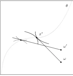
In order to have a closer look at what happens near a critical submanifold Ck, consider a trade curve x(·) crossing a C1 hypersurface S at some point x at time, say, T . Let the interior of the feasible set τ∗ be separated by S into domains G−and G+. The partial derivatives ∂ϕ
∂xk,
and ϕ+(x) be the limiting values of the function f at the point x ∈ S, from the domains G−
and G+ respectively. Let
h(x) := ϕ+(x) − ϕ−(x),
be the discontinuity vector at x of our vector field. Finally, let ϕ−N, ϕ+N, hN be the (orthogonal) projections of the vectors ϕ−, ϕ+, h onto the normal line to S directed from G− to G+ at
the point x. Within the domains G− and G+, right and left uniqueness of solution to (2)
holds true (Cauchy-Lipschitz theorem). All we therefore need is to study what happens in a neighborhood of the hypersurface S. The following Proposition summarizes the various situations we may encounter:
Proposition 4.4.1.— (Filippov21) If S is C2 and the function h(x) = f+(x) −
f−(x) is C1 at each point x ∈ S, if, moreover, at least one of the inequalities
fN−> 0 or fN+ < 0 (possibly different inequalities for different x) holds, the right uniqueness for (2) occurs for a < t < b in G.
A nice aspect of finitely subanalytic economies is that the set of economies for which our dynamics can be exactly simulated is certainly included in this family.22
How large is the class of finitely subanalytic economies ? If the space of initial endowments is taken to be the space of continuous maps ω : [0, 1] → τ , equipped with the uniform convergence, then density of finitely subanalytic endowment maps follows from the Stone-Weierstraß theorem. Regarding preferences, we take ω >> 0 as fixed, and equip the space of preferences restricted to τ and verifying (D) with the C2 topology.23
Proposition 4.4.2. Given ω >> 0, the set of preferences representable by a
finitely subanalytic utility is dense in the space of C2 utilities satisfying (D).
Proof. This follows from the standard proof showing that smooth preferences are dense
in the space of C2 utilities (see, e.g., Mas-Colell (1985, Prop. 2.8.1. p. 90)) by keeping track
of the fact that every object involved in the construction of the approximating sequence of smooth preferences must be finitely subanalytic. For this, one simply needs to observe that: (i) for any integer n > 0, a C∞-density function ξn: R`→ R with support containing the
origin and radius ≤ 1n can be constructed so as to be finitely subanalytic;
(ii) If v, ξn: R`→ R are finitely subanalytic, so is the restriction of the convolution
u0n(x) := Z
R
v(x − z)ξn(z)dz
to the compact τ . (Notice that the support of z in the integral is bounded.)
¤ The next examples illustrate the fact that (global) uniqueness of the strategy-proof trade curves obtains even though the set of Walras equilibria of the underlying economy may exhibit a strong indeterminacy.
Example 4.3.1. This time, suppose that u1(x, y) = u2(x, y) = x + y, ω1 = (2, 1), ω2 =
(1, 3). E is linear, and admits a continuum of Walras equilibrium allocations, all of them being Pareto-optimal. However, as we already saw, it admits a unique short-term price
P (L) = {(1, 1)}, and a unique short-term outcome: x∗
1 = (97,127 ), x∗2 = (127,167 ). The unique
21See Filippov (1968), Lemma 2 and Corollary 1 (p. 107), Corollary 2 and Lemma 3 (p. 108) and Theorem
2 (p. 110).
22This is also the family of economies to which the use of finite elements will lead, in order, say, to
ap-proximate weak solutions of our trajectories in the sense of the Ritz method (see, e.g., Zeidler (1991, p. 141).
23That is, the topology of uniform convergence over the compact τ of each uiand its derivatives up to order