HAL Id: cea-02567625
https://hal-cea.archives-ouvertes.fr/cea-02567625
Submitted on 7 May 2020
HAL is a multi-disciplinary open access
archive for the deposit and dissemination of
sci-entific research documents, whether they are
pub-lished or not. The documents may come from
teaching and research institutions in France or
abroad, or from public or private research centers.
L’archive ouverte pluridisciplinaire HAL, est
destinée au dépôt et à la diffusion de documents
scientifiques de niveau recherche, publiés ou non,
émanant des établissements d’enseignement et de
recherche français ou étrangers, des laboratoires
publics ou privés.
High-resolution, 3D radiative transfer modelling
Sam Verstocken, Angelos Nersesian, Maarten Baes, Sébastien Viaene, Simone
Bianchi, Viviana Casasola, Christopher J. R. Clark, Jonathan I. Davies, Ilse
de Looze, Pieter de Vis, et al.
To cite this version:
Sam Verstocken, Angelos Nersesian, Maarten Baes, Sébastien Viaene, Simone Bianchi, et al..
High-resolution, 3D radiative transfer modelling: II. The early-type spiral galaxy M 81. Astronomy and
As-trophysics - A&A, EDP Sciences, 2020, 637, pp.A24. �10.1051/0004-6361/201935770�. �cea-02567625�
A&A 637, A24 (2020) https://doi.org/10.1051/0004-6361/201935770 c ESO 2020
Astronomy
&
Astrophysics
High-resolution, 3D radiative transfer modelling
II. The early-type spiral galaxy M 81
Sam Verstocken
1, Angelos Nersesian
1,2,3, Maarten Baes
1, Sébastien Viaene
1,4, Simone Bianchi
5, Viviana Casasola
6,5,
Christopher J. R. Clark
7, Jonathan I. Davies
8, Ilse De Looze
1,9, Pieter De Vis
8, Wouter Dobbels
1, Frédéric Galliano
10,
Anthony P. Jones
11, Suzanne C. Madden
10, Aleksandr V. Mosenkov
12,13, Ana Trˇcka
1, and Emmanuel M. Xilouris
21 Sterrenkundig Observatorium, Universiteit Gent, Krijgslaan 281 S9 9000 Gent, Belgium
e-mail: [email protected]
2 National Observatory of Athens, Institute for Astronomy, Astrophysics, Space Applications and Remote Sensing,
Ioannou Metaxa and Vasileos Pavlou, 15236 Athens, Greece
3 Department of Astrophysics, Astronomy & Mechanics, Faculty of Physics, University of Athens,
Panepistimiopolis 15784, Zografos, Athens, Greece
4 Centre for Astrophysics Research, University of Hertfordshire, College Lane, Hatfield AL10 9AB, UK
5 INAF – Osservatorio Astrofisico di Arcetri, Largo E. Fermi 5, 50125 Firenze, Italy
6 INAF – Istituto di Radioastronomia, Via P. Gobetti 101, 4019 Bologna, Italy
7 Space Telescope Science Institute, 3700 San Martin Drive, Baltimore, MD 21218, USA
8 School of Physics and Astronomy, Cardiff University, Queen’s Buildings, The Parade, Cardiff CF24 3AA, UK
9 Department of Physics and Astronomy, University College London, Gower Street, London WC1E 6BT, UK
10 AIM, CEA, CNRS, Université Paris-Saclay, Université Paris Diderot, Sorbonne Paris Cité, 91191 Gif-sur-Yvette, France
11 Institut d’Astrophysique Spatiale, CNRS, Université Paris-Sud, Université Paris-Saclay, Bât. 121, 91405 Orsay Cedex, France
12 Central Astronomical Observatory of RAS, Pulkovskoye Chaussee 65/1, 196140 St. Petersburg, Russia
13 St. Petersburg State University, Universitetskij Pr. 28, 198504 St. Petersburg, Stary Peterhof, Russia
Received 25 April 2019/ Accepted 7 April 2020
ABSTRACT
Context.Interstellar dust absorbs stellar light very efficiently, thus shaping the energy output of galaxies. Studying the impact of different stellar populations on the dust heating continues to be a challenge because it requires decoupling the relative geometry of stars and dust and also involves complex processes such as scattering and non-local dust heating.
Aims.We aim to constrain the relative distribution of dust and stellar populations in the spiral galaxy M 81 and create a realistic model of the radiation field that adequately describes the observations. By investigating the dust-starlight interaction on local scales, we want to quantify the contribution of young and old stellar populations to the dust heating. We aim to standardise the setup and model selection of such inverse radiative transfer simulations so these can be used for comparable modelling of other nearby galaxies. Methods.We present a semi-automated radiative transfer modelling pipeline that implements necessary steps such as the geometric model construction and the normalisation of the components through an optimisation routine. We used the Monte Carlo radiative transfer code SKIRT to calculate a self-consistent, panchromatic model of the interstellar radiation field. By looking at different stellar populations independently, we were able to quantify to what extent different stellar age populations contribute to the heating of dust. Our method takes into account the effects of non-local heating.
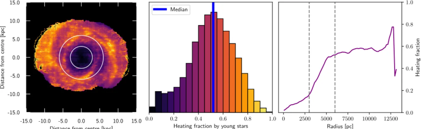
Results.We obtained a realistic 3D radiative transfer model of the face-on galaxy M 81. We find that only 50.2% of the dust heating
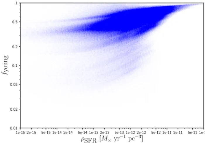
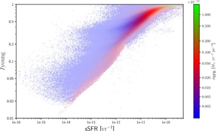
can be attributed to young stellar populations (.100 Myr). We confirm that there is a tight correlation between the specific star
formation rate and the heating fraction by young stellar populations, both in sky projections and in 3D, which is also found for radiative transfer models of M 31 and M 51.
Conclusions.We conclude that old stellar populations can be a major contributor to the heating of dust. In M 81, old stellar populations are the dominant heating agent in the central regions, contributing to half of the absorbed radiation. Regions of higher star formation do not correspond to the highest dust temperatures. On the contrary, it is the dominant bulge which is most efficient in heating the dust. The approach we present here can immediately be applied to other galaxies. It does contain a number of caveats, which we discuss in detail.
Key words. radiative transfer – dust, extinction – galaxies: individual: M 81 – galaxies: ISM – infrared: ISM
1. Introduction
Interstellar dust reprocesses optical and UV photons into infrared (IR) and submillimetre (submm) radiation. The line-of-sight extinction and reddening effects of dust in optical and UV wavebands in the Milky Way and other galaxies have provided us with crucial insights regarding the nature of absorption and scattering processes, as well as the dust grain
composition (Draine & Li 2007; Calzetti et al. 2000). On the other hand, observations at mid-infrared (MIR), far-infrared (FIR) and submm wavelengths have provided constraints on dust density, temperature, emissivity, and the correlation between the presence of dust and star formation. Since the advent of missions such as Spitzer (Werner et al. 2004) and Herschel (Pilbratt et al. 2010), it has become possible to study interstellar dust in hun-dreds of nearby galaxies on resolved scales. This has allowed the
relative properties for different regions of such galaxies in differ-ent environmdiffer-ents to be quantified. For a recdiffer-ent review on the interstellar dust properties in nearby galaxies, seeGalliano et al.
(2018).
Studies based on these data have shown that the diffuse, old stellar population in galaxies can play a significant role in the heating of interstellar dust (Hinz et al. 2004;Bendo et al. 2010,
2012,2015), whereas star formation can be attributed to most of the dust emission at shorter wavelengths, at, for example, 24 µm (Calzetti et al. 2005,2007;Prescott et al. 2007;Kennicutt et al. 2007, 2009; Zhu et al. 2008).Lu et al. (2014) find that, in the case of M 81, even at 8 µm and 24 µm, the old stars are respon-sible for 67% and 48% of the dust emission in the respective bands.
Nersesian et al. (2019) have investigated the dust-starlight interplay in 814 DustPedia1 galaxies across all Hubble stages
using the spectral energy distribution (SED) fitting code CIGALE (Boquien et al. 2019). They found that the relative con-tribution of young stellar populations (6200 Myr) to the dust heating is monotonically increasing with Hubble Stage, provid-ing – on average – only 10% of the absorbed energy in early-type galaxies up to 60% in the later type galaxies.
Using the global SED of a galaxy, however, only permits an average picture of the dust heating mechanisms within the galaxy. Therefore, the correlation between star formation and IR emission is stronger in certain regions of a galaxy, which is underestimated by the global fraction of heating by young stars as indicated by the global SED model. Moreover, global SED models assume dust absorbs light from either stellar population independent of their relative spatial distribution. Differences in heating fraction between galaxies, therefore, are the direct result of the relative amount of young and old stars required to explain the UV-NIR part of the galaxy spectrum and how these intrinsic stellar spectra vary as a function of position over the galaxies.
To take into account the geometry of stellar and dust com-ponents, SED fitting tools can also be used on resolved scales by fitting the spectrum on a pixel-by-pixel basis. This requires a panchromatic dataset defined on a uniform coordinate grid. These methods have proven useful for studying local varia-tions in star formation, dust density, dust characteristics, etc. (Galliano et al. 2011; Gordon et al. 2014; Viaene et al. 2014;
Decleir et al. 2019). However, SED fitting still has its limita-tions in this context, as each pixel is treated independently. This approach neglects the fact that depending on the inclination, the line-of-sight probes different regions in the galaxy, which poten-tially bear different stellar and dust properties. More importantly, enforcing a local energy balance does not take into account the propagation of radiation over lengths greater than the physical scale of the pixels. This non-local character of dust heating might be important (Smith & Hayward 2015;Boquien et al. 2015). 3D radiative transfer analyses have demonstrated the non-locality of dust heating in the Sombrero galaxy (De Looze et al. 2012a) and the Andromeda galaxy (Viaene et al. 2017). In both galaxies, the radiation from the old stellar populations in the bulge has proven to propagate far outwards and contribute to the heating out to large distances.
To include these non-local dust heating effects, we require a self-consistent 3D model of the galaxy that fully incorporates the effects of scattering, absorption, and dust emission. Upon
1 DustPedia (Davies et al. 2017;Clark et al. 2018) is multi-wavelength
survey of galaxies in the Local Universe. The DustPedia sample consists of 875 nearby galaxies (recessional velocities of <3000 km s−1) with
Herscheldetection and angular sizes of D25> 10.
bearing the cumulative effect of these physical processes, the photons must be propagated back into the line-of-sight to make a proper comparison to observed galaxies possible. Thus, a 3D panchromatic radiative transfer (RT) model is required to obtain a realistic description of the stellar and dust distribution (see
Steinacker et al. 2013for an overview of RT codes and descrip-tion of the techniques).
The procedure described above, where the 3D stellar and dust compositions are simultaneously constrained by fitting the emergent radiation field to observed data of a galaxy, is referred to as inverse 3D radiative transfer or 3D radiative transfer modelling. Up to now, most attempts at RT model entire galaxies focused on edge-on spiral galaxies and typically adopt axial symmetry (e.g.Xilouris et al. 1999; Bianchi 2008;
Baes et al. 2010; Popescu et al. 2011; Schechtman-Rook et al. 2012;De Looze et al. 2012b,a;Mosenkov et al. 2016,2018). In their RT study of M 51,De Looze et al.(2014) introduced novel techniques for the modelling of well-resolved face-on galaxies, and effectively marked the onset of full 3D radiative transfer modelling. The main advantage of using face-on galaxies is that the filamentary and spiral features observed in the disc can be directly used for the geometric model construction, whereas for edge-on galaxies only 2D axially symmetric, smooth discs can be assumed. The use of these heterogeneously mixed geome-tries, along with the inclusion of multiple UV components, allow for a much more realistic analysis of the interaction between stel-lar radiation and the interstelstel-lar matter, which reduces the dust energy balance problem (Saftly et al. 2015).
This work is a continuation and extension of the analysis car-ried out byDe Looze et al.(2014) and it is also aimed at setting up a strategy for a systematic radiative transfer modelling effort of a larger sample of nearby galaxies (e.g.Nersesian et al. 2020;
Viaene et al. 2020). Within the scope of DustPedia (Davies et al. 2017), with consistency and reproducibility in mind, we have bundled the modelling tools into a software package that is specifically aimed at convenient future use and designed in a way to make it capable of tackling a larger sample of face-on galaxies. In this work, we describe this modelling approach and apply it to the early-type spiral galaxy M 81 (c3031, Sab, Hubble stage= 2.4, D ≈ 3.7 Mpc, i ≈ 59 deg). M 81 is an interacting galaxy (e.g. Casasola et al. 2004), belonging to the M 81 group consisting of 34 members. The gas content of M 81 has been extensively studied (e.g. Combes et al. 1977;
Sakamoto et al. 2001; Casasola et al. 2007;Heiner et al. 2008;
Sánchez-Gallego et al. 2011) because of the strong density wave attributed to the tidal interaction with the companions of the M 81 group, especially M 82 and NGC 3077 (Kaufman et al. 1989).
This paper is structured as follows. In Sect.2, we describe how the multi-wavelength image data for M 81 were gathered and prepared for our model construction and verification. In Sect.3, we describe in detail our updated approach for the setup of a 3D radiative transfer model of face-on galaxies and show the specific properties of the model of M 81. The results of the M 81 modelling are described in Sect.4, which includes the verifica-tion of the model based on its SED and an investigaverifica-tion in the dust heating mechanisms. In Sect.5, we discuss the implications of our modelling results as well as the limitations and caveats in our modelling approach. Our conclusions are given in Sect.6.
2. Data collection and preparation
For M 81, imaging data are available from all of the seven tele-scopes that gather data as part of DustPedia (GALEX, SDSS,
2MASS, WISE, Spitzer, Herschel, and Planck). This gives us 35 images which are automatically retrieved from the DustPedia archive2by the modelling pipeline. For an overview of the pixel scales, FWHMs, and calibration uncertainties for the DustPedia images, seeClark et al.(2018). In addition to the images that are part of the sample, a continuum-subtracted Hα image is retrieved from NED3, based on the study byHoopes et al.(2001).
We removed stars from GALEX, SDSS, and Spitzer IRAC images with an automatic procedure developed as part of the modelling pipeline and also described briefly in Clark et al.
(2018). The procedure, in broad terms, consists of the follow-ing steps. First, the 2MASS All-Sky Catalog of Point Sources (Cutri et al. 2003) is queried for the coordinate range of the particular image. The catalogue data is accessed through the Vizier interface of the A
stroquery
package (Sipocz 2016), anA
stropy
affiliated package (Astropy Collaboration 2018). Foreach position in the catalogue, we looked for a local peak above a 3-sigma significance level. Non-detections mean that the par-ticular catalogue position is ignored. The local background is then subtracted from the neighbouring pixels of each remaining point source position and they are fitted to a 2D Gaussian pro-file. If that fitting is successful, a segmentation step is performed to detect saturation bleed, diffraction patterns, and ghosts typ-ically found around the brightest stars. The flagged pixels are then interpolated over by replacing them by a weighted aver-age of the neighbouring pixels that are not flagged and then they are complemented with random noise mimicking the variation in these pixels. A manual inspection is performed afterwards and the procedure is repeated with mistakenly identified point sources ignored or additional regions flagged for interpolation.
All images are corrected for background emission and sys-tematic offsets by estimating the large-scale variation of pixel values around the galaxy. We use the mesh-based background estimation tools from P
hotutils
(Bradley et al. 2018). In this method, the image is divided up into a grid of rectangular regions where the local background is estimated, then this grid is upsam-pled to the original pixel resolution. We have chosen square boxes with a side of six times the FWHM of the image. All pixels identified as belonging to the galaxy (as an elliptical region) are masked, as well as all pixels flagged during the source extrac-tion as being either a foreground star or a background galaxy. To estimate the sky and its standard deviation behind the galaxy, the maps resulting from the Photutils
upsampling method are interpolated within the central galaxy ellipse.Images affected by Milky Way attenuation must be cor-rected by a factor that depends on the filter response curve and a galactic extinction law (Cardelli et al. 1989). We calcu-late the attenuation in all wavebands <10 µm by convolving a Rλ
curve with RV = 3.1 with the corresponding filter transmission
curves obtained from the SVO Filter Profile Service4, and using
the I
rsa
Dust
tool of Astroquery
(querying the IRSA Dust Extinction Service5) to obtain the V-band attenuation AVfor the
galaxy position (Schlafly & Finkbeiner 2011). This step is also automated within the modelling pipeline.
For Spitzer and Herschel images, error maps are avail-able from the DustPedia archive, derived from their respective data reduction pipelines. To assert uniformity across our multi-wavelength dataset, however, we opt to generate the error maps independently with our modelling pipeline. In general, the error
2 http://dustpedia.astro.noa.gr
3 https://ned.ipac.caltech.edu
4 http://svo2.cab.inta-csic.es/svo/theory/fps/
5 https://irsa.ipac.caltech.edu/applications/DUST/
map for a certain band is a combination of three contributions: the calibration uncertainty, pixel-to-pixel noise estimated from the deviation from the smooth background, and Poisson noise. The pixel-to-pixel noise is the deviation of the pixel values from the assumed smooth background, which is produced during the sky subtraction step. The Poisson noise is taken into account for photon-counting instruments where the number of detected pho-tons in an individual pixel can be low. We create Poisson error maps for the GALEX and SDSS images. Creating these maps is not trivial, as the DustPedia GALEX and SDSS images are the result of a mosaicking of individual observations. In the case of GALEX, we have to take into account a variable exposure time for each observation. For SDSS, the observations (fields) have to be recalibrated from nanomaggy units into photon counts, taking into account the 2D polynomial sky that has been subtracted by the SDSS imaging pipeline and a different calibration factor per image column. The pixel noise and Poisson noise (where appli-cable) are added in quadrature with the calibration error map for each band. The relative calibration errors for each band are listed in Table 1 ofClark et al.(2018).
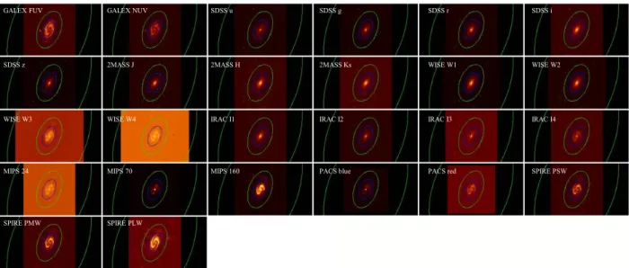
Global photometry is applied to each clipped image by sum-ming all pixels within a fixed elliptical aperture with semi-major and semi-minor axes of 72700. 7 and 42100. 2, respectively. An
overview of the different images with the apertures for the inte-grated flux determination and the annuli for the determination of the background is provided in Fig.1. We selected this aperture to exclude extended emission that is present in some images and the satellite dwarf galaxy Homberg IX that is most prominent in the UV bands. Corresponding uncertainties are also calculated by adding the calibration uncertainty and the mean variation from the background in quadrature. The resulting flux densities, listed in the table in the Appendix, differ only slightly from the Dust-Pedia photometry (on average, our fluxes are about 2% lower). The detection of M 81 in the Planck images is extremely faint compared to the Galactic cirrus, or even indistinguishable from it, which is why our HFI 100 GHz, HFI 143 GHz, and LFI fluxes are taken as the upper limits. The Planck images and fluxes are not used to construct the RT model and thus only serve the pur-pose of making visual comparisons.
3. Modelling approach
3.1. General outline
In this section, we present a general overview of our mod-elling strategy. We present a detailed description in Sect.3.2and Sect.3.3. We present our optimisation strategy in Sect.3.4.
The general modelling approach that we apply is the follow-ing. We construct a 3D model for the galaxy, consisting of sev-eral stellar components and a dust component. More specifically, we consider four different stellar components: a central bulge of old stars, an old stellar disc, a young non-ionising stellar disc, and a disc with an even younger stellar population (the young ionising disc). This standard model with three distinct stellar age categories is illustrated in Fig.2.
The geometrical distribution of each of the components is based on observed images of the galaxy at different wavelengths using a two-step procedure. The first step consists of combining different images to physical maps that characterise, for exam-ple, the distribution of dust or old stellar populations on the sky. The second step consists of de-projecting these 2D maps on the sky to a 3D distribution. Apart from the geometrical distribution, each stellar component is assigned an intrinsic SED, and a total luminosity that is either fixed or a free parameter in the model.
GALEX FUV GALEX NUV SDSS u SDSS g SDSS r SDSS i
SDSS z 2MASS J 2MASS H 2MASS Ks WISE W1 WISE W2
WISE W3 WISE W4 IRAC I1 IRAC I2 IRAC I3 IRAC I4
MIPS 24 MIPS 70 MIPS 160 PACS blue PACS red SPIRE PSW
SPIRE PMW SPIRE PLW
Fig. 1.Photometry thumbnail image grid for M 81. The blue ellipse in each image is the master ellipse used for the determination of the integrated
flux. The green ellipses mark the annulus used for the determination of the background.
old population
young non-ionising population
young ionising population
2D cut perpendicular to the disc
Fig. 2.Standard geometric model of spiral galaxies adopted in our
mod-els. The old stellar population consists of a disc and bulge component. The young stellar population is assumed to be restricted to the disc and consists of a non-ionising subpopulation with an age around 100 Myr, and an ionising subpopulation of stars with an age of 10 Myr. The young non-ionising population resides in a thinner disc compared to the old stars, and the young ionising population is even more compacted to the mid-plane of the galaxy. The dust distribution exhibits the same vertical extent as the young non-ionising stellar population.
Similarly, the optical properties of the dust component are spec-ified, and the total dust mass is a free parameter in the model.
For any choice of the three free parameters in the galaxy model, we can set up a 3D dust radiative transfer simulation that fully takes into account the emission by the different stellar populations, and the absorption, scattering and thermal emission by the dust. These simulations are performed with SKIRT, a general-purpose dust radiative transfer code based on the Monte Carlo technique (Baes et al. 2011;Camps & Baes 2015) that is publicly available6. The challenging 3D galaxy simulations we
run here are possible thanks to the large suite of input models (Baes & Camps 2015), the advanced grid structures (Saftly et al. 2013, 2014), the optimisation techniques (Steinacker et al. 2013;Baes et al. 2016), and the hybrid parallelisation strategies (Verstocken et al. 2017) implemented in SKIRT.
The result of each such simulation is a well-sampled 3D (x, y, λ) cube from which we extract the SED and a set of broad-band images of the galaxy. These images, from UV to submm wavelengths, can directly be compared to the observed images. The best fitting model is determined through a χ2 optimisa-tion procedure: using a two-step grid-based fitting approach,
6 http://www.skirt.ugent.be
we determine the free parameters of the model that reproduces the observed SED best. As soon as the best fitting model is determined, a wealth of possible information can be extracted. For example, additional images of the galaxy at arbitrary view-ing points and arbitrary wavelengths can be calculated, and the intrinsic properties of the interaction between starlight and dust can be studied in 3D.
In general, our modelling procedure largely follows the same approach asDe Looze et al.(2014) andViaene et al.(2017), but with some improvements and important differences. One major distinction is that we construct all the components in the model at their “native” resolution, in the sense that we no longer re-bin and convolve all input images to the same resolution before we use them to construct our stellar and dust components. Instead, we ensure that we match the resolution of each particular set of images that is used for a specific map and in this way we allow for the highest possible resolution for each particular compo-nent. Another difference is the computation of a pixel-by-pixel goodness-of-fit metric across all bands instead of solely using fluxes from the integrated SED.
Overall, we have taken special care to automate the entire procedure as much as possible. The different steps in the proce-dure, discussed in the following subsections, are implemented in Python and are publicly available as part of the Python Toolkit for SKIRT (PTS)7. This automation and open-science approach
has the obvious advantage that our results can immediately be reproduced or extended by other teams, along with the fact that the same approach can easily be applied to other galaxies. In the subsections below, we provide more details on the different modelling steps, complemented by aspects that are specific to the model of M 81.
3.2. The different components in the model 3.2.1. The stellar bulge
The stars and dust in a spiral galaxy are distributed in a flat-tened disc, with the exception of a central bulge that con-sists primarily of old stellar populations (e.g.Alton et al. 1998;
Bianchi 2007; Muñoz-Mateos et al. 2009; Hunt et al. 2015;
Casasola et al. 2017). The first step in the modelling procedure is therefore to set up a suitable model for the bulge. The old stellar population can be best seen in NIR wavebands, where the contri-bution from recently formed stars is usually limited, the contam-ination from dust emission is negligible, and internal extinction by the dust is also modest.
The Spitzer Survey of Stellar Structure in Galaxies (S4G:
Sheth et al. 2010;Salo et al. 2015) has provided a database of decompositions in Spitzer IRAC 3.6 and 4.5 µm bands for 2352 nearby galaxies. The bulges of the galaxies are usually mod-elled as flattened Sérsic models, and the decomposition param-eters can be retrieved from an ASCII table provided on the S4G
pipeline webpage8.
The 2D Sérsic surface brightness distribution is de-projected to a 3D intrinsic distribution under the assumption that the bulge has an oblate spheroidal distribution and the inclination of the bulge is the same as the inclination of the old stellar disc (we assume that all components have the same inclina-tion). The SKIRT code is equipped with a dedicated routine (SersicGeometry) that constructs a 3D spheroidal bulge model based on the characteristics of the Sérsic surface brightness dis-tribution and the inclination. The spatial density and cumula-tive mass distribution can be expressed analytically using special functions (Baes & Gentile 2011;Baes & van Hese 2011).
The setup of a stellar component is not complete until the intrinsic spectrum and the normalisation are defined. For the old stellar population in the bulge, we adopt a Bruzual & Charlot
(2003) spectral energy distribution with a fixed metallicity and an age of 8 Gyr. These numbers are similar to the values used byViaene et al.(2017) for the bulge of M 31, but they can obvi-ously be changed if this information is available for the particular galaxy to be modelled. The old stellar age of 8 Gyr is a middle ground between 5–13 Gyr, the common range for old stellar pop-ulations. In fact, the actual SEDs don’t change too much within this age range.Kong et al.(2000) find a super-solar metallicity of 0.03 for M 81 that is rather uniform across the galaxy, which is therefore the value we adopt for the stellar components of our M 81 model.
The total bulge luminosity is fixed by the total IRAC 3.6 µm flux density from the bulge as obtained from the best fitting S4G model, and this luminosity is assumed to be unaffected by inter-nal dust attenuation and thus can be directly used as the intrinsic normalisation of the bulge component.
For the specific case of M 81, the S4G team have found a
best-fitting Sérsic model for the bulge with a Sérsic index n = 3.56, an effective radius of 1.38 kpc, an axial ratio (flattening) of 0.654, and a position angle of 55 degrees (Salo et al. 2015). The IRAC 3.6 µm flux density of the bulge is 5.31 Jy, corresponding to a luminosity of
Lbulge, 3.6= 2.11 × 1035W µm−1. (1)
We use SKIRT to render an image of the bulge using the SersicGeometry and arbitrary normalisation to obtain a 2D image of the bulge component on the plane of the sky. This image is shown in the first panel of Fig.3.
3.2.2. The old stellar disc
A map of the old stellar population in the disc of the galaxy can be obtained by subtracting the bulge (as resulting from the decom-position) from the total observed image in the IRAC 3.6 µm band. With the technique introduced by De Looze et al. (2014) and
8 http://www.oulu.fi/astronomy/S4G_PIPELINE4/MAIN/
implemented in SKIRT’s ReadFitsGeometry, we can directly load this 2D map into SKIRT which converts it into a 3D disc component. De-projections such as these are generally degener-ate and require some assumptions to generdegener-ate a unique solution. We resolve the degeneracy by imposing that the old stellar disc has a perfectly exponential distribution in the vertical direction, with a fixed scale height (actually, we make the same assumption for all the disc components, with a separate scale height for each com-ponent) (Wainscoat et al. 1989,1990;van der Kruit & Freeman 2011). The method works by mapping each pixel in the image to a position in the mid-plane of the 3D model, implying a rota-tion over the posirota-tion angle and essentially a stretch of the image along the direction of the minor axis with a factor of cos i. The direct mapping from plane of the sky to plane of the galaxy makes the implicit assumption of an infinitely thin disc, but it is also a reasonable approximation for low inclination angles.Viaene et al.
(2017) have even achieved realistic de-projection results for M 31 with an inclination angle of 77.5◦. We base our estimated
incli-nation angle for M 81 on the apparent flattening of the disc found by the S4G decomposition, using the Hubble formula
(Hubble 1926): sin2i= 1 − q 2 1 − q2 0 · (2)
An important parameter is the exponential scale height of the disc. Various studies of edge-on disc galaxies have found quite strong correlations between the scale height of the stellar component and other properties, including the stellar disc scale length, total luminosity, and rotational velocity (e.g. de Grijs 1998; Kregel et al. 2002; Bianchi 2007; Courteau et al. 2007). We use the results obtained byDe Geyter et al.(2014) based on detailed radiative transfer modelling of 12 edge-on spiral galax-ies. They found a mean intrinsic flattening, that is, a ratio of scale length to scale height, of 8.26. This value is almost exactly the same as the value obtained byKregel et al.(2002) based on independent surface brightness model fitting of 34 edge-on spiral galaxies. Our strategy is thus to take the scale length as obtained from the S4G bulge-disc decomposition, and use that to compute
a value for the scale height of the old stellar disc.
Finally, we generally assume the same stellar population (an SSP of 8 Gyr and a fixed metallicity) as for the old population of the bulge and we fix the total luminosity based on the fitted disc luminosity from the S4G exponential disc fit. For the specific case of M 81, the old stellar disc map is shown in Fig.3. From S4G, we find a scale height of 332 pc and a total IRAC 3.6 µm
luminosity slightly higher than that of the bulge:
Ldisc, 3.6= 2.20 × 1035W µm−1. (3)
Using the intrinsic flattening q0 = 1/8.26 and an apparent
axis ratio of 0.543, formula (2) yields the inclination angle i = 57.8◦.
3.2.3. The young non-ionising stellar disc
Apart from old stellar populations, galaxies also contain recently formed stars. These stellar populations constitute a minor frac-tion of total stellar mass, but as they dominate the emission at blue and UV wavelengths, they play a crucial role in the heat-ing of the interstellar dust and, thus, in our RT models. Similar toDe Looze et al.(2014) andViaene et al.(2017), we separated the young stellar population into two subpopulations. The main subpopulation, which we denote as the young non-ionising pop-ulation, corresponds to stars that have formed about 100 Myr ago
55m 56m 57m +68◦540 +69◦000 060 120 180 Dec (J2000)
Old stellar bulge
55m
56m
57m
Old stellar disc
55m 56m 57m RA (J2000) Young non-ionising stellar disc 9h55 m 56m 57m Young ionising stellar disc 9h54 m 55m 56m 57m Dust disc
Fig. 3.2D view of the different model components, including a bulge and disc component for the old stellar population, discs of young
non-ionising and non-ionising stellar populations, and the disc of the dust distribution. The bulge image has been rendered with SKIRT by using the 3D bulge description and the appropriate instrument setup. The disc component maps have been produced with recipes directly using the observed multi-wavelength images, as detailed in the text. The different maps have different native resolutions based on the respective observations that were used to create these maps. These resolutions are 100.9 for the old stellar bulge and disc, 1100.2 for the young non-ionising stellar disc, 600.4 for
the young ionising stellar disc, and 1100.2 for the dust disc (see Table1). The removal of unphysical pixels due to different signal-to-noise in each
of the bands leads to a varying contour for the different components. and that have already left their birth clouds. The second subpop-ulation, which we denote as the young ionising popsubpop-ulation, cor-responds to stars formed within the last 10 Myr, which are there-fore assumed to be still embedded in their birth clouds, heating it by their hard ionising radiation. Splitting the young population into these two disc subcomponents allows for dust in clumpy regions, (perhaps) not picked up in attenuation from the diffuse stars, but still contributing emission due to the contained star-formation activity. In fact, this clumpy dust will be incorporated as a sub-grid feature, as discussed in Sect.3.2.4. Hence, this method guards against energy balance problems without neces-sarily imposing a fixed fraction of young stars to be ionising or introducing artificial clumping in the dust geometry.
The population of young stars that are no longer obscured by their birth clouds of gas and dust can be expected to dominate the emission in the FUV band and, to a lesser extent, the NUV band, although there may be a significant contribution from the older stellar population, certainly in the inner regions. Addition-ally, FUV radiation is very efficiently absorbed and scattered (attenuated) by dust and therefore the intrinsic luminosity of the young non-ionising stellar population is not directly related to the observed FUV flux density.
The first step in the construction of an intrinsic 3D model for the distribution of the young non-ionising stellar population con-sists of making a map of the intrinsic FUV emission. To create this map, we combine the observed FUV surface brightness map with an estimate of the FUV attenuation map. This attenuation map is set up using the prescriptions ofCortese et al.(2008), who have performed a regression of the FUV attenuation as a poly-nomial function of the logarithm of the total infrared (TIR) to FUV ratio, on spatially resolved scales. The coefficients of the polynomial are determined for different values of the specific star formation rate (sSFR). Following the prescriptions described in
Galametz et al.(2013), we determine a TIR emission map based on the MIPS 24 µm, the PACS 70 µm, and the PACS 160 µm images. SPIRE band images are not included in the creation of the TIR map because it would drastically degrade the resolution of the resulting map. Different UV-to-optical/NIR colours provide good
estimators of the sSFR on global or resolved scales. When avail-able, we prefer the FUV − r colour, as the r band image usually combines a high resolution with a high signal-to-noise. Based on this colour map, we create a sSFR map (which is smoothed by convolving it with a kernel with twice the FUV FWHM to elimi-nate noise), and this map is used in combination with the TIR and FUV maps to determine the FUV attenuation and intrinsic (unat-tenuated) FUV emission maps.
Subsequently, we correct this intrinsic FUV map for the contribution from old stars by subtracting a scaled version of the 3.6 µm image from this map. We determine the best scal-ing factor based on the assumption that the contribution from star formation in the bulge-dominated region is minimal. Hence, we define an elliptical region that corresponds to the bulge-dominated region of the galaxy and determine, for each scaling factor, the relative number of pixels that have a negative value in that region of the subtracted map. We take 10% as the upper limit of negative pixels that the corrected map can have so that the subtraction still makes physically sense (assuming 10% neg-ative values are largely due to noise). After the subtraction, a smoothing is applied to interpolate over the negative values. We refer, for instance, toLeroy et al.(2008),Rahman et al.(2011),
Cortese(2012),Ford et al. (2013),Casasola et al. (2017) for a similar analysis.
This intrinsic young non-ionising stellar population FUV map is de-projected to a 3D disc model using the ReadFitsGeometry routines in SKIRT, in the same way as discussed for the old stellar population map. Following
De Looze et al. (2014) we use the same scale height for this population as for the dust, that is, half of the scale height of the old stellar population (see Sect.3.2.5).
Finally, we assign an intrinsic spectral energy distribu-tion and a normalisadistribu-tion to this component. Again, we use a
Bruzual & Charlot(2003) SSP model, with the same metallic-ity as for the old stars, but now with an age of 100 Myr. The normalisation, that is, the total luminosity, is left as a free param-eter in the model. The resulting young non-ionising stellar disc of M 81 is shown in Fig.3.
Table 1. Summary of the maps used for the radiative transfer model and their properties, as well as the observed images that have used to produce each map.
Component Images used Pixel scale FW H M
[arcsec] [arcsec]
Old stellar disc IRAC 3.6µm 0.75 1.9
Young non-ionising disc GALEX FUV, IRAC 3.6 µm, SDSS r, MIPS 24 µm, PACS 70 µm, PACS 160 µm 4.0 11.2
Young ionising disc MIPS 24µm, IRAC 3.6 µm, Hα 2.03 6.43
Dust SDDS r, GALEX FUV, MIPS 24 µm, PACS 70 µm, PACS 160 µm 4.0 11.2
Notes. The image with the lowest resolution, thus determining the resolution of the map, is indicated in bold.
3.2.4. The young ionising stellar disc
The presence of very young, partially obscured stars can be traced by Hα emission, which unfortunately is again affected by attenuation. Using a sample of 33 nearby galaxies,Calzetti et al.
(2007) present a prescription to create an extinction-corrected Hα map, based on the observed Hα map and the MIPS 24 µm map,
SHα, corr= SHα+ 0.031 S24. (4)
We first correct the observed 24 µm image for a contribution from the old stellar population that may also emit at these wave-lengths, using a similar approach as discussed for the contribu-tion of old stars to the FUV emission. We use this corrected 24 µm image and the Hα image, convolved and re-binned to the same resolution, and use the equation above to obtain the map of the young ionising stellar component, shown in Fig.3. This map is again de-projected in the same way, with a scale height that is half the value of the scale height of the young non-ionising stellar population, that is, a quarter that of the old stellar disc (Viaene et al. 2017).
For the young ionising stellar population, we adopt the SED templates for obscured star formation from Groves et al.
(2008), based on 1D simulations of Starburst99 SSP models (Leitherer et al. 1999) and the photoionisation modelling code MAPPINGS III (Groves et al. 2004). The result of their mod-elling is a suite of templates defined on a five-dimensional grid of the metallicity of the gas (Z), the mean cluster mass (Mcl), the compactness of the clusters (C), the pressure of the
surrounding ISM (P0), and a fraction controlling the optical
depth of the gas and dust for the UV photons ( fPDR). The
nor-malisation of the templates scales with the star formation rate (SFR). We used the following parameters as our default values: Z = 0.03, Mcl = 105M , log C = 6, P0/k = 106cm3K, and
fPDR = 0.2. Similar values have been used by De Looze et al.
(2014) and Viaene et al.(2017) in their radiative transfer mod-elling of M 51 and M 31 and in other studies that used these MAPPINGS III SEDs as templates for star forming regions in galaxy-wide simulations (e.g.Camps et al. 2016;Trayford et al. 2017;Camps et al. 2018). All template SEDs are implemented in SKIRT for immediate use in combination with any kind of geom-etry. Finally, the normalisation of the young ionising stellar disc component, meaning the total luminosity, is a free parameter in the modelling.
3.2.5. The diffuse dust disc
The final component to be considered is the dust disc. A map of the dust surface mass density can be obtained directly from the FUV attenuation (De Looze et al. 2014). For M 81, the dust map, shown in Fig.3, shows some interesting features. Two clear
spiral arms are visible, coinciding with those found for the young stellar populations, yet the center of the galaxy is mostly devoid of dust. Such a depression of the dust surface density is found in many DustPedia galaxies (Mosenkov et al. 2019). A secondary spiral pattern is visible in the inner region, as already noted by
Connolly et al.(1972) andDevereux et al.(1997).
The dust map is de-projected by SKIRT to a 3D dust dis-tribution, assuming a dust scale height that is half that for the old stellar population. This value is driven by the results of detailed radiative transfer modelling of edge-on spiral galax-ies (Xilouris et al. 1999; Bianchi 2007; De Geyter et al. 2014;
Mosenkov et al. 2018).
For the dust composition, we use the THEMIS9 dust mix
appropriate for the diffuse ISM (Jones et al. 2017). The model is calibrated to reproduce the dust emission and extinction with a mixture of amorphous carbonaceous grains and silicate grains. The total dust mass, Mdust, which acts as the normalisation
con-stant for the dust distribution, is a free parameter of the model. Table 1 gives an overview of the different components in the RT model that are constructed based on a 2D map and de-projected. Their intrinsic resolutions, depending on the used observational images, are also listed in this table.
3.3. Set up of the SKIRT simulations
Based on the input maps and a minimum set of additional input parameters, our PTS pipeline creates the maps and 3D com-ponents necessary for the SKIRT radiative transfer modelling, and it also automatically generates the SKIRT parameter file (for details on and an example of a SKIRT parameter file, see
Camps & Baes 2015. Before a simulation can be run, a number of additional settings need to be chosen.
The spatial resolution of a SKIRT radiative transfer model is defined by the discretisation of the dust component in the so-called dust grid. The density and other dust properties are therefore constant within each unit of the grid (dust cell), and during the SKIRT simulation, all photon packages are propa-gated across this grid. The stellar emission is sampled on the input resolution of the stellar component maps. To accommo-date the complexity of the structure in the dust distribution and limit the required computing resources as much as possible, we use the built-in binary tree grid structure in SKIRT (Saftly et al. 2014), which constructs the grid in a hierarchical way by split-ting cells alternately along the three axis planes. The minimum and maximum subdivision levels are chosen to be 6 and 36, respectively, and we set the stopping criterion for individual cells to the point where they contain less than 5 × 10⁻⁷of the total dust mass (Saftly et al. 2013). This threshold is similar to val-ues used in the previous SKIRT simulations of spiral galaxies
(De Looze et al. 2014; Saftly et al. 2015; Camps et al. 2016,
2018;Viaene et al. 2017;Trayford et al. 2017).
For the specific case of M 81, the total extent of the dust grid is 26 kpc in the x and y direction, and 3.32 kpc in the vertical direction. The maximum level of 36 subdivisions corresponds to a maximum spatial resolution of 26 kpc/212 = 6.36 pc, or 0.36 arcsec at the distance of M 81. As a result of the mass fraction criterion, the subdivision was truncated after level 27, such that the effective resolution was 50.9 pc, or equivalently 2.84 arcsec. In total, SKIRT generated a dust grid with 2.9 lion cells; the leaves of a hierarchical tree consisting of 5.8 mil-lion individual nodes.
Another important aspect of any SKIRT simulation is the choice of the wavelength grid. SKIRT uses a fixed wavelength grid, in the sense that only photon packages with specific wave-lengths are used in the simulation. For the choice of the spe-cific wavelength grid in our modelling, several criteria are taken into account. On the one hand, the number of wavelengths needs to be restricted since the run time of a single simulation scales in a roughly linear fashion with the number of wavelengths. On the other hand, the different input stellar SEDs and the expected dust emission SEDs need to be properly covered, while sharp emission and absorption features need to be resolved, and the different broadband filters need to be properly sampled to allow for a proper convolution with the filter curves. A more detailed description of the wavelength grid construction is given in AppendixB. Balancing accuracy and computational feasibil-ity, we settle on 250 wavelength points distributed in a non-uniform way over the entire UV-mm wavelength range.
Finally, we simulate data cubes of the observed radiation. For the M 81 model, we choose the characteristics of the data cubes with a pixel scale of 4 arcsec or 71.6 pc, and a field of view of 17.9 × 31 kpc. This yields data cubes of 250 × 433 × 250 = 27.1 million individual pixels. The instrument is placed at the galaxy distance of 3.69 Mpc, with the inclination angle of 57.8◦ and position angle of 66.3◦also assumed for the de-projection.
3.4.χ2optimisation
The best-fitting values for the remaining free parameters in the RT model are determined through a χ2optimisation procedure.
In the setup described above, we have three free parameters: the dust mass Mdust, the FUV luminosity of the young non-ionising
stellar disc Lyni, FUV, and the FUV luminosity of the young
ionis-ing stellar disc Lyi, FUV. We note that the luminosity of the bulge
and the old stellar disc are not free parameters in the model because their normalisation is based on the 3.6 µm emission, which is relatively free of dust attenuation or contamination by young stellar populations. It is obviously possible to adapt this scheme and consider these luminosities as additional free param-eters, or to include other free parameters such as the galaxy incli-nation or the dust optical properties if that would be required or interesting for the specific galaxy or the scientific questions to be addressed.
Initial guesses for the free parameters are determined through SED fitting results from (Nersesian et al. 2019), per-formed with the CIGALE (Boquien et al. 2019). For most of the nearby galaxies within the DustPedia sample, CIGALE SED fitting has been performed, and the results are available on the DustPedia archive. For this purpose, the THEMIS dust model was introduced into CIGALE, a delayed and truncated SFH has been assumed (Ciesla et al. 2016), and for the SSPs the
Bruzual & Charlot(2003) spectra are used. Various parameters are derived from the best fitting stellar and dust population mix,
including the SFR, the stellar and dust mass, the FUV attenua-tion and the temperature of the dust. We convert this SFR into a spectral luminosity for the young ionising stellar component by generating theGroves et al.(2008) spectrum with the appropri-ate model parameters and scale it to the obtained star formation rate. Subsequently, we take the observed FUV luminosity, cor-rect it with the FUV attenuation value found by CIGALE, and subtract the found FUV luminosity of the young ionising popula-tion to get the intrinsic luminosity of the young non-ionising stel-lar component. Finally, the dust mass from CIGALE is directly used as our initial guess for the dust mass in the SKIRT mod-elling. For the case of M 81, the total dust mass according to this CIGALE fit and, hence, the initial guess for our SKIRT modelling, is:
Mdustinit = 9.61 × 10⁶M . (5)
The SFR obtained for M 81 is 0.351 M yr−1, and applying the
recipes as described above yield the following initial guesses for the FUV luminosities of the young ionising and non-ionising stellar discs:
Linityi, FUV= 1.59 × 1036W µm−1, (6) Linityni, FUV= 3.18 × 1036W µm−1. (7) We then need to optimise our model parameters going from the initial guess to a set that best represents the observations. As these fully-3D panchromatic Monte Carlo radiative transfer simulations are computationally demanding, it is important to limit the total number of simulations. Because we restrict the number of free parameters in our optimisation to only three, the problem at hand is still conveniently solvable with a brute-force parameter grid evaluation method. We follow a two-step approach where we first test the parameter space around our ini-tial guess with faster simulations and then refine the parameters with detailed simulations.
We determined the best fitting radiative transfer model parameters evaluating the χ2 metric. For the first, exploratory
grid, we compared the global fluxes of the model to the observed integrated SED of M 81: χ2=X X wX Fsim X − F obs X σobs X 2 , (8)
where FXsim, FobsX and σobsX are the global mock flux density, observed flux density, and observed error corresponding to band X, respectively. The differential weight factors wX were chosen
such that each wavelength regime has an equal importance (see alsoViaene et al. 2017). We defined six different regimes (ionis-ing, young, old, mix, aromatic, and thermal dust). Each of these regimes was chosen to reflect the presumed dominating contri-bution of a particular model component, and, thus, the regime where this component is most likely to be best constrained. We assigned an equal weight to each of the regimes since we wanted all model components to be equally well-constrained, and deter-mined the weight factor for the filters in a regime based on their count10.
10 We selected the filters from the GALEX, SDSS, Spitzer, WISE and
Herscheltelescopes, but we also avoided filters that are too close in
effective wavelength. In particular, we generally chose IRAC 3.6 µm
over WISE 3.4 µm, IRAC 4.5 µm over WISE 4.6 µm, and MIPS 24 µm over WISE 22 µm. This yields a set of 18 filters to be used for the fitting.
For the second, detailed grid, we compute the χ2 metric based on the pixel-by-pixel difference of observed versus mock images in each band:
χ2=X X X p wX µsim X (p) − µ obs X (p) σobs X (p) 2 . (9)
The first summation covers all filters X for which data are available, the second sum loops over all pixels p in the image corresponding to band X. The quantities µsim
X (p), µ obs X (p) and
σobs
X (p) are the mock surface density, observed surface density,
and observed error in pixel p of band X, respectively. Finally, wX is again a differential weight factor given to the band X,
as in Eq. (8). The choice for a local χ2 can be computation-ally demanding. Generating mock images with sufficiently high signal-to-noise in all pixels and in all bands requires for each model takes considerable computation time. The average CPU time in this phase of the M 81 modelling was 311 h for each simulation11. Depending on the level of detail and available resources, it is also possible to fall back to the global χ2in this
step. This was done for M 31, for example, which is more than seven times larger than M 81 (seeViaene et al. 2017). We note that this will become less of a problem as soon as the recently released new version of SKIRT (SKIRT 9:Camps & Baes 2020) has been fully validated. In this new version of the radiative transfer code, mock broadband images are directly generated as part of the simulation. Instead of producing large data cubes with many of small wavelength bins, the relevant photon packages of a particular band are captured directly and stored in a much smaller data cube of broadband images. This is a more time- and memory-efficient way of making mock images, which can subse-quently be used to minimise the χ2per pixel. The reduced χ2
val-ues are converted into probabilities as exp(−12χ2) and the proba-bilities of all models with a certain parameter value are summed to yield the probability of that particular parameter value.
The exploratory grid as a test of our initial guess is set as a coarse, yet broad grid in the (Mdust, Lyni, FUV, Lyi, FUV) parameter
space. We consider five grid points for the dust mass and for the FUV luminosity of the young non-ionising disc, both on a log-arithmic grid. Dust masses are generally reasonably well con-strained by SED fitting, so we chose a range for the dust mass parameter of just one order of magnitude around the initial value. The young non-ionising stellar disc FUV luminosity is harder to constrain, so we chose two orders of magnitude for this param-eter. Based on the analysis for M 31 (Viaene et al. 2017), we assume that the normalisation of the young ionising stellar disc is generally even harder to constrain, so we conservatively use a broader grid of seven points for this parameter, spanning three orders of magnitude around the initial guess. Still, the ranges are chosen with the idea that one can always expand them if borders are hit. In total, the first batch contains 175 radiative transfer simulations.
As indicated above, we sped up the evaluation in this step by reducing the output detail (the simulation’s internal 3D resolu-tion remains the same). For the simularesolu-tions in this exploratory grid, we generate a lower-resolution wavelength grid of just 115 wavelengths, abandoning the requirement of spectral convo-lution and thus only including the effective wavelength of each filter for a direct comparison to observation. We also do not cre-ate the full data cube for each simulation but let SKIRT crecre-ate a global simulated SED. In this step, we use 106photon packages
per wavelength, which is sufficient for generating SEDs. These
11 All simulations together consumed around 107 000 CPU hours.
adaptations provide almost an order of magnitude in speedup, but still 34 h of CPU time were required per simulation.
Based on the results of this initial grid of models, we create a finer grid centred around the expected values of the free parame-ters. This time we use seven grid points in each of the dimen-sions of the (Mdust, Lyni, FUV, Lyi, FUV) parameter space,
result-ing in 343 additional simulations. In these simulations, we use five times as many photon packages and employ the full high-resolution wavelength grid. We create a data cube for each sim-ulation and spectrally convolve this cube to create a mock image for each observed filter. We subsequently re-bin these images to the coordinate system of the corresponding observed image and clip them to the same field-of-view. We can thus evaluate the χ2measure on a per-pixel basis (Eq. (9)). This large
compu-tational effort is preferred over the minimisation of a global χ2 (Eq. (8)) because it also captures local variations between model and observation. The impact of using a global χ2is discussed in AppendixD.
3.5. Summary of the modelling steps
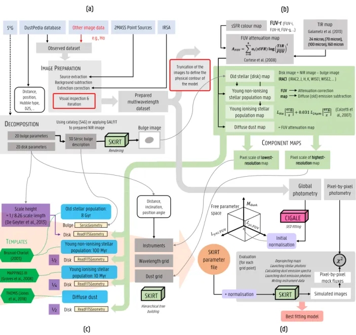
Figure4 summarises outlines the general 3D radiative transfer modelling approach we adopted and which will also apply for our future work. It shows the key steps that are involved in the modelling, such as the image preparation, the map making, the decomposition, and the fitting steps.
4. Results
4.1. Model selection and properties
The probability distributions from the 175 simulations of the first set of models for M 81 are shown in red in Fig.5. For the dust mass and the FUV luminosity of the young non-ionising stel-lar disc, the expected value is the initial guess value. For the FUV luminosity of the young ionising stellar disc, the grid point with the highest probability is 5.02 × 1035W/µm, one grid point below the initial guess value. This shows that models deviat-ing significantly from the initial guess values are punished by a higher global χ2. Following this test grid, we can be confident
of our setup and thus run the more detailed simulations of the more narrow, but better sampled, parameter grid. The resulting probability distributions are over-plotted in blue in Fig.5. Also indicated are the parameter values of the best fitting simulation (lowest local χ2). The most probable values (peak of the blue
distributions) of the parameters are:
Mdust = (1.28 ± 0.27) × 107M , (10)
Lyni, FUV= (4.24 ± 1.43) × 1036W µm−1, (11)
Lyi, FUV= (5.02 ± 4.78) × 1035W µm−1. (12)
The most likely radiative transfer model for M 81, i.e. the model with the lowest local χ2, has the following parameters:
Mdust = 1.28 × 10⁷M , (13)
Lyni, FUV= 3.18 × 1036W µm−1, (14)
Lyi, FUV= 1.59 × 1036W µm−1. (15)
The model with these parameter values is the one we adopted for the rest of the analysis.
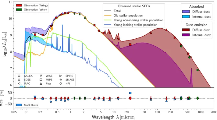
4.2. Spectral energy distribution
The simulated SED of the best fitting model is shown in Fig. 6, along with the observed photometry derived from the
Observed dataset
DECOMPOSITION
DustPedia database Other image data
S4G 2MASS Point Sources IRSA e.g., Hα
Using catalog (S4G) or applying GALFIT to prepared NIR image 2D bulge parameters 2D disk parameters Bulge image (a) SKIRT 3D Sérsic bulge description Rendering sSFR colour map
Old stellar (disk) map
Young ionising stellar population map Diffuse dust map
FUV-r(FUV-i, FUV-H, FUV-g, …)
Disk image = NIR image – bulge image IRAC1 (IRAC2, J, H, K, WISE1, WISE2, … )
= FUV attenuation map
24 micron, (70 micron), (100 micron), 160 micron Galametz et al. (2013) TIR map (Calzetti et al., 2007) FUV map Attenuation correction Diffuse (old) emission subtraction
Young non-ionising stellar population map
(b) COMPONENT MAPS Instruments Diffuse dust Scale height = 1 / 8.26 scale length (De Geyter et al., 2013)
½ Bruzual-Charlot (2003) MAPPINGS III (Groves et al., 2008) THEMIS (Jones et al., 2018) TEMPLATES Wavelength grid SersicGeometry ½ ¼
Old stellar population: 8 Gyr
Young non-ionising stellar population: 100 Myr
Young ionising stellar population: 10 Myr (c) Bulge ReadFITSGeometry Disk ReadFITSGeometry Disk ReadFITSGeometry Disk ReadFITSGeometry Disk
Pixel scale of highest-resolution map Pixel scale of
lowest-resolution map
Deprojecting maps Launching stellar photons Calculating dust emission spectra Launching dust emission photons
Writing instrument data
Free parameter space Evaluation (for each grid point) Pixel-by-pixel mock fluxes (d) SKIRT parameter file Hierarchical tree building Distance, inclination, position angle SKIRT
Best fitting model Prepared multiwavelength dataset SKIRT Dust grid SED fitting Global photometry Initial normalisation CIGALE
+ normalisation Simulated images
Source extraction Background subtraction
Extinction correction Visual inspection &
iteration IMAGEPREPARATION Distance, position, Hubble type, D25, … Truncation of the images to define the
physical contour of the model
Cortese et al. (2008)
FUV attenuation map
Pixel-by-pixel photometry
Fig. 4.Semi-automatic modelling approach, as implemented in the Python code PTS. Indicated in red are steps that require manual intervention.
At the top of the diagram, the different input sources are displayed. These include the DustPedia archive, but also other image data can be included in the modelling environment. The images are prepared uniformly by the pipeline, using the 2MASS point sources catalogue and IRSA service for dust extinction. If Spitzer 3.6 µm or 4.5 µm data is available, a 2D decomposition is retrieved from the S4G catalogue; or else custom decomposition
parameters can be specified. The prepared images are used to obtain a map of the different stellar and disc components based on well-established
prescriptions. What is crucial in the map-making process is the FUV attenuation map which, in turn, is based on an sSFR colour map (the preferential colour is indicated in bold, though other colours can be used depending on the availability and quality of the data) and a TIR map
(created by combining multiple MIR/FIR bands with a consideration of the resolution). The maps and 3D bulge description define the geometry
of the RT model, together with appropriate scale heights for each of the disc components. The RT model is further defined by a wavelength grid, an instrument setup, and a dust grid. Given this basic model, SKIRT is used to determine the best normalisations of stellar and dust components.
For more details, we refer to the main text in Sect.3. (a) Preparation and decomposition, (b) map making, (c) model construction, and (d) model
normalisation (fitting).
prepared images. The total model SED is represented by the black line starting from the left side of the spectrum, taken over by the red line where the dust emission adds to the stellar part of the model SED on the longer wavelength side of the panel. Overall, the simulation reproduces the observa-tions notably well. A direct comparison on a global scale is shown in the bottom panel of Fig. 6, where the reference is the observation (red points for the bands included in the fitting, green points for other observed fluxes). The mock fluxes (blue points) are derived from the simulated luminosity’s by spectrally
convolving them with the appropriate filter transmission curves and applying the same aperture photometry as we performed on the observations. Residual percentages are defined as (model– observation)/observation.
The most prominent deviation of the model from the obser-vation is seen for the MIPS 24 µm band (50%). This band lies close to the peak of the hot dust component related to the ionis-ing stellar populations. It seems that on a global scale, our model overestimates this contribution. It is important to note that mod-els with lower Lyi, FUV did not provide a better fit to the data.
2.0 5.0 10.0 20.0 Mdust [M ] (×106) No rmalised probabilit y best model 0.2 0.5 1.0 2.0 5.0 10.0 20.0 Lyni, FUV [W/µm] (×1036) 0.5 1.0 2.0 5.0 10.0 20.0 50.0 100.0 200.0 500.0 Lyi, FUV [W/µm] (×1035)
Fig. 5.Probability distributions of the RT models for the first batch (red) and the second batch of simulations (blue). From left to right: diffuse
dust mass, the FUV luminosity of the young non-ionising disc, and the FUV luminosity of the young ionising stellar disc. For the second run, the values of the overall best-fitting simulation are indicated by the vertical lines.
6 7 8 9 10 11
log
10λL
λ[L
]
GALEX SDSS IRAC WISE MIPS Pacs SPIRE 2MASS HFI Observation (fitting) Observation (other)Observed stellar SEDs
Total
Old stellar population
Young non-ionising stellar population Young ionising stellar population
Absorbed Diffuse dust Internal dust Dust emission Diffuse dust Internal dust 0.05 0.1 0.2 0.5 1 2 5 10 20 50 100 200 500 1000 2000
Wavelength λ [micron]
−50 0 50Res.
[%]
Mock fluxesFig. 6.Top panel: panchromatic SED corresponding to the SKIRT radiative transfer model for M 81. The total observed stellar energy output is
indicated with a black line and the total dust emission, when added to the stellar spectrum, follows the red line. The area shaded in purple above the observed stellar spectrum represents the radiation that is absorbed by the diffuse dust, thus the purple line represents the intrinsic stellar spectrum. Yellow, green, and dark blue lines represent the contribution of the old, the young non-ionising, and the young ionising stellar populations to the observed stellar spectrum, respectively. The area shaded in light blue above the young ionising population curve indicates the absorbed energy by internal (subgrid) dust. The area shaded in magenta between 20 and 500 µm indicates the energy distribution emitted by this internal dust. Bottom panel: comparison between the observed fluxes and the simulated SED, as relative residuals with the observations as reference. Observed fluxes are shown as red and green points, depending whether or not they were used in the fitting procedure. The blue points show the mock fluxes derived from the simulated SED.
While reducing the MIPS 24 µm emission, they lower the MIR continuum entirely and thus producing a higher χ2. In compar-ison, the WISE 22 µm flux (not shown, but see Table A.1) is 10% higher than the MIPS 24 µm emission. Part of this discrep-ancy may also be related to instrumental uncertainty in the MIR. The residuals for the other bands are at maximum 25% and usu-ally lower. The 2MASS and Planck fluxes were not included for the fitting procedure because of significant large-scale sky noise and poor spatial resolution, respectively. Nevertheless these also agree well with the model (5%).
4.3. Image comparison
Spectral convolution of the simulated data cubes for the 18 bands (used for fitting) gives rise to a set of mock images for every
model of the second batch of the fitting procedure. A selection of such images, clipped to the observed high signal-to-noise mask, for the best fitting simulation is shown in Fig.7. Here, the first column shows the observations and the second column the mock images. Because model and observation are generally difficult to discriminate, we highlight the small-scale relative differences through residual maps, shown in the third column. The last col-umn shows the probability density distribution of the residual pixel values. In Fig.8, we additionally show the corresponding radial profiles derived from the residual maps.
In the NUV band there is an overall good agreement with most deviant pixels well below 100%. The largest offsets occur in the inter-arm regions. Here the model over-estimates the flux as part of the applied deprojection of the 2D input maps. In the bulge the model slightly underestimates the UV flux. As such
GALEX NUV −100 0 100 Residual (%) SDSS g −100 0 100 Residual (%) Observation IRA C 3.6 µ m Model Residuals −100 0 100 Residual (%) 100 50 0 -50 -100 Mips 24 µ m −100 0 100 Residual (%) P A CS 160 µ m −100 0 100 Residual (%) Observation SPIRE 500 µ m Model Residuals −100 0 100 Residual (%) 100 50 0 -50 -100
Fig. 7.Comparison between observed and simulated images in 6 different wavebands. First column: observed images. Second column: mock
images, created by spectrally convolving the simulated data cube. Third column: maps of the relative residuals between observed and mock images. Last column: distributions of the residual pixel values. The mock images are clipped to the same pixel mask as the observed images. The probability density functions of the residuals are calculated with a kernel density estimation (KDE).
0
2
4
6
8
10
R (kpc)
40
20
0
20
40
60
80
100
Re
sid
ua
l (
%
)
GALEX NUV
SDSS g
IRAC I1
MIPS 24 m
PACS 160 m
SPIRE 500 m
Fig. 8.Median residual versus galactocentric radius derived from the
residual maps in Fig.7. Each waveband is assigned with a different
colour indicated in the upper left corner of the figure.
there’s a rising trend of residual percentage with galactocentric radius. The pixel distribution is more narrow in the g band, where model and observed image look very similar, giving rise to a flat radial profile. There is however a global offset of ∼25% as already noted in the previous section. The main factors influ-encing the optical SED fit are the stellar populations and the dust attenuation. Since the offset in the g band is uniform across the disc, the latter is unlikely responsible. Instead, this may be caused by insufficient resolution in the star formation history of our simulation (modeled by the three stellar population ages). A fourth component with an age between 100 Myr and 8 Gyr, or alternatively a stellar component with a continuous range of ages, could alleviate the offset in global flux while maintaining the smooth residual map.
In the NIR, there is a narrow residual distribution as well. The IRAC 3.6 µm pixels follow the observations closely. A weak
radial trend is visible where low-luminosity disk pixels are are slightly overestimated and bulge pixels tend to be underesti-mated by the model. The good agreement in this band confirms our assumptions that the young stellar populations have no rel-evant contribution to the emission and that dust attenuation is insignificant here.
The situation is considerably worse in the MIPS 24 µm band, where the model typically generates pixel fluxes that are too high (see also Sect.4.2). The corresponding radial profile in Fig.8
shows a steep rise from negative percentages in the centre to pos-itive residuals beyond 1 kpc. The residuals keep increasing out-wards, but at a slower rate. This band was used in combination with Hα to construct the surface density map of the young ion-ising component (Eq. (4)). It is possible that this empirical pre-scription is introducing the radial trend in the residuals obvious in Fig.8. In addition the emission template for the young ionis-ing component has several tuneable parameters that can produce relatively higher 24 µm emission. We unfortunately do not have sufficient observational constraints to explore this vast parameter space. For consistency comparability, we adopted the same val-ues as other radiative transfer model of this kind (De Looze et al. 2014;Viaene et al. 2017;Williams et al. 2019).
The only regions where the 24 µm flux is underestimated by the model are the very centre of M 81 and the clumpy star form-ing regions in the spiral arms. The latter is seen in other bands as well, yet mostly where star formation is prominent (for example in the UV). The origin of this blurring is twofold, partly show-ing the effects of de-projection and its assumptions, yet another important degradation in resolution comes from the fact that multiple bands are combined into the input maps of the model components. For the 24 micron band, for instance, the observed image has a resolution (FWHM) of 6.43 arcsec, but the simu-lated emission map is modusimu-lated by the dust map which has a resolution of 11.18 arcsec (as does the young non-ionising stel-lar map), even though this dust is heated by the young ionis-ing population (FW H M = 6.43 arcsec) as well. As a result of our choice of retaining the maximal resolution for each compo-nent separately, the resolution of the resulting data cube is the