HAL Id: hal-01647790
https://hal.archives-ouvertes.fr/hal-01647790
Submitted on 24 Nov 2017
HAL is a multi-disciplinary open access
archive for the deposit and dissemination of
sci-entific research documents, whether they are
pub-lished or not. The documents may come from
teaching and research institutions in France or
abroad, or from public or private research centers.
L’archive ouverte pluridisciplinaire HAL, est
destinée au dépôt et à la diffusion de documents
scientifiques de niveau recherche, publiés ou non,
émanant des établissements d’enseignement et de
recherche français ou étrangers, des laboratoires
publics ou privés.
turbulence
Quentin Aubourg, Antoine Campagne, Charles Peureux, Fabrice Ardhuin,
Joël Sommeria, Samuel Viboud, Nicolas Mordant
To cite this version:
Quentin Aubourg, Antoine Campagne, Charles Peureux, Fabrice Ardhuin, Joël Sommeria, et al..
Three-wave and four-wave interactions in gravity wave turbulence. Physical Review Fluids, American
Physical Society, 2017, 2 (11), �10.1103/PhysRevFluids.2.114802�. �hal-01647790�
Quentin Aubourg,1 Antoine Campagne,1 Charles Peureux,2 Fabrice
Ardhuin,2 Joel Sommeria,1 Samuel Viboud,1 and Nicolas Mordant1, ∗
1
Laboratoire des Ecoulements G´eophysiques et Industriels (LEGI), Universit´e Grenoble Alpes, CNRS, F-38000 Grenoble, France
2
Laboratoire d’Oc´eanographie Physique et Spatiale (LOPS), Univ. Brest, CNRS, Ifremer, IRD, F-29200 Plouzan´e, France
The Weak Turbulence Theory is a statistical framework to describe a large ensemble of nonlinearly interacting waves. The archetypal example of such system is the ocean surface that is made of interacting surface gravity waves. Here we describe a laboratory experiment dedicated to probe the statistical properties of turbulent gravity waves. We setup an isotropic state of interacting gravity waves in the Coriolis facility (13 m diameter circular wave tank) by exciting waves at 1 Hz by wedge wavemakers. We implement a stereoscopic technique to obtain a measurement of the surface elevation that is resolved both in space and time. Fourier analysis shows that the laboratory spectra are systematically steeper than the theoretical predictions and than the field observations in the Black Sea by Leckler et al. JPO 2015. We identify a strong impact of surface dissipation on the scaling of the Fourier spectrum at the scales that are accessible in the experiments. We use bicoherence and tricoherence statistical tools in frequency and/or wavevector space to identify the active nonlinear coupling. These analyses are also performed on the field data by Leckler et al. for comparison with the laboratory data. 3-wave coupling are characterized and shown to involve mostly quasi resonances of waves with second or higher order harmonics. 4-wave coupling are not observed in the laboratory but are evidenced in the field data. We finally discuss temporal scale separation to explain our observations.
∗
I. INTRODUCTION
The Weak Turbulence Theory (WTT) is a statistical theory that describes the evolution of an ensemble of interacting non-linear waves (wave turbulence). Applicable to a wide variety of dispersive waves (for reviews, see [1–3]), the theory has been historically developed in the 60’s by Zakharov [4] in plasma physics and Hasselmann in oceanography for the modeling of surface gravity waves [5]. The application of the theory relies on two asymptotic hypotheses: the domain must be large and non-linearities weak. Thus, a scale separation appears between the linear time of the wave TL = 2π/ω and the typical slow non-linear time TN L related to the non-linear waves interactions. As the
non-linearity is weak, only resonant interactions are able to develop a long time coupling and then transfer energy. The resonant conditions impose that the wave vector ki and the frequencies ωifollow:
k1= k2+ k3 ω1= ω2+ ω3 (1)
at the lowest order that involves 3-waves interactions. The number N of waves in an interaction is generally set by the order N − 1 of the non-linear term in the dynamic equations. Thus, for surface water waves for which the non-linear term is quadratic, we expect N = 3. However N is also ruled by the existence or the absence of geometrical solutions to the resonant equations. For freely propagating waves, these solutions can be found using the linear dispersion relation of the waves. For surface gravity waves, the negative curvature of the dispersion relation ω =√gk does not allow for resonant waves with N = 3, and N = 4 should be considered.
k1+ k2= k3+ k4 ω1+ ω2= ω3+ ω4. (2)
In the following, when using the words “N-wave resonance”, we mean a set of Fourier modes (ω, k) that fulfills the resonance equations (1) or (2) independently of whether the Fourier mode corresponds to an actual freely propagating wave (ie following the linear dispersion relation) or not. In particular it may include bound waves generated by quadratic nonlinearities. This is somewhat different to the meaning used most often in the oceanographic community, namely what we call 3-wave interaction that involves a bound component is usually referred to as a 4-wave interaction. The WTT relies on these resonant equations and allows to solve analytically the temporal evolution of statistical quantities in several physical systems. In the situation of an out of equilibrium and stationary forced system, it leads to the so-called Kolmogorov-Zakharov (KZ) power spectrum [1]. For gravity waves, since the dispersion relation follows a unique power law, solutions can be found as well using dimensional analysis [2]. It leads to the following prediction for the spectrum of the surface elevation η: Eη(k) ∝ g−1/2P1/3k−5/2 where k = kkk, g is the gravity and
P is the average injected power. The exponent 1/3 = 1/(N − 1) is related to the 4-wave resonance. Using the linear dispersion of surface gravity waves ω = √gk, it is then possible to express the spectrum in the frequency space : Eη(ω) ∝ gP1/3ω−4.
Although gravity waves are among the pioneering systems for the study of non-linear waves interactions, laboratory observations show a strong variability. Unlike capillary waves-assemblies for which the WTT predictions of the spectral exponent seem consistent with the observations [6–10], spectra of pure gravity waves are often in contradiction with the WTT and show a forcing-dependent power spectrum. The spectral exponent predicted by the WTT is actually observed only for strongly forced systems, which is obviously inconsistent with the major hypothesis of weak nonlinearity [7, 11–13], whereas the exponent is significantly steeper than the prediction in the weak non-linearity limit. The main reason that is generally proposed to explain these discrepancies is a failure of the condition of an asymptotic large system or the presence of overturning waves. As experiments have always a finite size, a discretization of the k-space appears and may not allow to satisfy the resonant conditions [14]. These discrete effects can be overcome when non-linearities increase: non-linearity induces a finite spectral width of the modes and may allow quasi-resonant interactions between waves that are not strictly on the linear dispersion relation [15, 16]. However, this situation is often in contradiction with the second hypothesis of weak non-linearities if too strong linearities are required to overcome the discreteness of the modes. A second cause for the observed differences with the WTT predictions may be attributed to the presence of dissipation in the inertial range where the energy cascade is operating. It generates a leak of energy and tends to steepen the power spectrum of the waves and thus decrease the spectral exponent as it has been observed for flexural wave turbulence [17, 18]. It is well known that surface waves are very sensitive to interface pollution that forms a very thin layer of organic material at the surface (oil, surfactants,...). Due to the presence of an elastic pollution film at the surface, the stress boundary conditions are changed compared to the ideally clean case and the induced boundary layer is considerably more dissipative [19]. The pollution layer is deformed by fluctuations of the surface, and it is subject to compressive waves [20]. These waves, referred to as Marangoni waves, are the main cause of dissipation of surface waves through the boundary layer with a maximal efficiency at frequencies close to 4 Hz, at which a resonance appears between the dispersion relations of surface gravity waves and Marangoni waves [19, 21]. The addition of these two effects are most likely responsible for the difference between the observed wave power spectrum and the WTT predictions.
The goal of the present article is thus to investigate directly the wave interactions that are at the core of the theory. We perform an analysis of high order correlation similar to that presented in previous investigations of surface gravity-capillary wave turbulence [22, 23]. The experimental setup is presented in the part II. A first analysis of the power spectrum and the effect of the pollution is detailed in part III. Then 3-wave and 4-wave resonant interactions are investigated in part IV and V.
II. EXPERIMENTAL SETUP
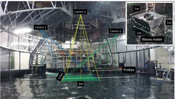
FIG. 1. Picture of the experimental setup : waves are generated by vertical oscillations of two wedge wavemakers of size 1m × 1m × 1m (visible in the inset). The deformation of the interface is measured in space and time using three cameras
positioned above the surface. The common field of view of the cameras covers a surface of 2 × 1.5 m2
. We seed the surface with polystyrene buoyant particles of 0.7 mm diameter. We perform cross-correlation between the different views in order to reconstruct the interface deformation η(x, y, t) as well as the velocity field u = (u, v, w) [24]. A set of four capacitive probes are also used to obtain single point measurements.
Figure 1 shows the general setup of the experiment. Gravity waves are generated in a 13 m diameter circular tank filled with fresh water at a rest height equal to 70 cm. In order to restrict surface pollution, the water surface is cleaned using a skimmer (see figure 2): the upper water layer flows in a 1 m cylinder connected to an intermediate tank located below the main one. The water is then pumped through a active carbon filter before being re-injected at the surface of the wavetank. The filtration is operated during a few hours in order to obtain the cleanest water surface. Waves are generated using two vertically oscillating wedge wavemakers of size of about 1 × 1 × 1 m3 and
placed at roughly 1.5 m from the wall (Fig. 1). They are driven within a range of (2 − 4) cm in amplitude and with a randomly modulated oscillation frequency centered around 1 Hz. The modulation follows a Gaussian distribution of width 0.15 Hz. The curved walls provide an efficient mixing of the waves and a rather homogeneous state is observed. Two methods are implemented to measure the surface deformation: a local one with four capacitive probes and a time and space-resolved scheme using three cameras located about 4 m above the free surface. In the latter case, called Stereo-PIV in the following, buoyant particles are seeded at the surface in order to form a random pattern which is recorded simultaneously by the cameras. A cross-correlation between the three cameras at the same time is first computed to reconstruct the free surface using a stereoscopic algorithm. In a second step, a PIV (Particles Images Velocimetry) measurement is performed that provides the velocity field in the framework of each cameras. We finally merge all the PIV fields by using the stereoscopic reconstruction that allows us to combine correctly the velocity components of distinct cameras at the deformed surface of water. In this way we obtain a complete 2D resolved velocity field at the free surface (see [24] for details of the image processing). In the “classical” Stereo-PIV technique the velocity is reconstructed in the bulk of the fluid in a flat plane illuminated by a laser sheet. Here the velocity field is computed at the surface of water which is not flat and it makes the reconstruction algorithm quite different. For simplicity we still refer to our method as Stereo-PIV. The main reason for implementing this global
FIG. 2. Setup used to clean up the free surface: the upper water layer flows in a 1 m cylinder located near the wall of the circular tank and connected to an intermediate tank located below the main one. The water is then pumped through an active carbon filter before being reinjected at the surface at a location diametrically opposite to the skimmer.
method instead of using only the stereo surface reconstruction is the improvement of the dynamical range of the measurement by measuring directly the power spectrum of the speed which is mathematically shallower than the one computed from the stereo (the former being the spectrum of a velocity and the latter of the elevation). We found a gain of about one order in magnitude in energy [24]. The knowledge of the velocity field also allows us to directly measure the non linear advective term as it will be presented below in part III.
The stereoscopic method allows us to reconstruct the free surface elevation η over a field of view of about 2 × 1 m2 with a vertical sensibility close to 0.6 mm [24]. The spatial resolution is restricted by the inhomogeneous seeding of the particles. We used polystyrene particles with a diameter of 0.7 mm. Due to well known capillary effects, a depression of the free surface is created between particles that generates an attraction that can act over a distance greater than 10 diameters [25, 26]. For very weak waves, the particle dispersion by the waves is not efficient enough to balance this tendency to coalesce and thus we are not able to reduce the PIV correlation window below a size of 30 pixel, which corresponds to a horizontal resolution of 4 cm.
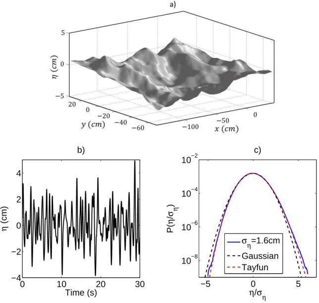
Figure 3(a) shows a snapshot of the spatial reconstruction of η and Fig. 3(b) an example of the temporal evolution at one location. Figure 3(c) displays the distribution of η normalized by the standard deviation wave height ση =
ph(η2i = 1.6 cm (assuming hηi = 0). We observe a slight deviation from the Gaussian distribution. Our observation
is better described by the Tayfun distribution [27] simplified by Socquet-Juglard et al. [28] :
P (η) = 1 − 7σ2 ηk 2 p 8 p2π(1 + 3G + 2G2)exp(− G2 2σ2 ηk2p ) G =p1 + 2kpσηη − 1 (3)
where kp is the wavenumber of the maximum peak in the power spectrum. This correction suggest the presence
of harmonic waves (2nd order) over a Gaussian linear field as it is commonly observed in gravity wave experiments [13, 29]. We thus suspect the presence of significant nonlinearities in our experiment.
0
10
20
30
−4
−2
0
2
4
b)
η
(cm)
Time (s)
−5
0
5
10
−810
−610
−410
−2c)
η
/
σ
ηP(
η
/
σ
η)
σ
η=1.6cm
Gaussian
Tayfun
FIG. 3. (a) Snapshot of the 3D reconstruction of the free surface elevation η(x, y, t). (b) Temporal evolution of η at one given
location in the image. (c) Probability density function of η normalized by the standard deviation of the wave height ση= 1.6 cm.
The dashed black line is the normal distribution. The red dashed line is the Tayfun distribution which incorporates non-linear second order effects (see text).
III. SPECTRAL ANALYSIS
1. Single point spectra and water pollution
FIG. 4. Two pictures of the free surface taken prior to the filtration (left) and after filtering during a few hours. The intensity of the forcing is equivalent for both case. The filtration change significantly the surface and capillary waves become present.
We begin with the analysis of the data recorded by the capacitive probes in a large variety of regimes to investigate the influence of water pollution. A strong sensitivity to the filtering of the water surface has been found. Figure 4 compares two pictures of the free surface before and after the filtration under identical forcing conditions. Before the filtration (Fig. 4(a)), the free surface is smooth. This suggests the presence of a strong dissipation of short waves. Shortly after stopping the filtration (Fig. 4(b)), the wave field looks very different with numerous short capillary waves riding on the crest of longer waves.
A quantification of these visual differences is obtained by computing the frequency power spectrum Eη(ω) =
h|η(ω)|2i estimated from the capacitive probes. η(ω) is the Fourier transform in time over a given time window and the average h·i is a temporal average over successive time windows. Figure 5(a) shows two power spectra corresponding to two experiments with similar steepness (but slightly distinct forcing intensity) in which data was recorded either before (red curve) or after filtration (blue curve). As expected by the visualization of the free surface, the power spectrum obtained with a filtered surface shows an exponent close to −5 whereas the exponent is about −8 for polluted water that corresponds to a much steeper spectrum. Figure 5(b) shows several measurements of α obtained by fitting a power law in a range of wavevectors where the spectrum is behaving as a power law. The fitting range is usually quite narrow, between ω/2π = 2 Hz and ω/2π = 5 Hz at best. The spectral exponent is shown as a function of the typical wave steepness ǫp which is a usual quantification of the intensity of non-linearities. As no direct
measurement of the wave steepness is possible with a local measurement, an estimation from the power spectrum is used : ǫp = 2kpση where kp is the wave number of the principal peak of the power spectrum (same definition as in
[29]). A good agreement (within 10%) with the direct measurement ǫ = p(∂η/∂x)2+ (∂η/∂y)2 has been checked
with the spatial reconstruction : ǫp ≈ σǫ = phǫ − hǫii2 (where the slope is averaged in time and space to obtain
hǫi). Although both estimates are aimed at quantifying the typical slope, such a good quantitative agreement is most likely a coincidence rather than a general rule. Dark triangles are measurements reported by Deike et al. [12] in a 15 × 10 m2 wave tank (similar size than ours but with a rectangle shape rather than circular). Blue and red
squares are our measurements with and without the filtration. A good matching with the measurements of Deike et al. [12] is observed, showing that Deike’s experiments are also most likely impacted by surface pollution. However, even with the filtration, the theoretical exponent α = −4 given by the WTT is not reached at low wave steepness. This suggests that the filtration may not be efficient enough and that a residual pollution remains and steepens the spectra. Nonetheless the surface dissipation has clearly being strongly reduced by filtration as the spectral exponent increases when cleaning the water surface. Another possibility is that finite size effects that may be dominant. Yet,
10
−110
010
110
−510
0E
η(
ω
)
ω
/2
π
(Hz)
a)
Prior to filtration
After the filtration
α
=−8
α
=−5
0
0.1
0.2
0.3
0.4
−14
−12
−10
−8
−6
−4
−2
b)
α
ε
pDeike et al. 2015
Prior to filtration
After the filtration
Leckler et al. 2015
FIG. 5. (a)Temporal power spectrum Eη(ω) for two experiments with a similar wave steepness. The red curve is obtained
without filtration of the free surface while the blue is obtained after a few hours of filtration. The exponent of the spectrum changes from about −8 initially to −5 for the cleanest water. (b) Distribution of the measured spectral exponent α as
function of the typical steepness of the waves ǫp(changed by tuning the magnitude of the forcing). Dark triangles are previous
measurements reported by Deike et al. [12]. The blue and red squares are respectively our measurements with and without filtration. The single purple point is an in-situ measurement of gravity waves in the Black sea [30].
these measurements emphasize that great care must be taken in order to minimize the problem of water pollution that affects the power spectrum in a major way. And this even for a gravity wave experiments where the large scales of the experiment may lead one to believe to be insensitive to surface contamination. Indeed, the maximum of dissipation occurs near 3 Hz which correspond to a wavelength of about 15 cm for a linear wave. To obtain one decade in frequency of waves that are unaffected by this pollution, we would need to force waves at 0.1 Hz with a wavelength of about 150 m. So even in our large wave tank, we cannot ignore this pollution. This condition can be fulfilled in Nature as shown by the data point (purple in Fig. 5(b)) extracted from Black Sea data by Leckler et al.. The nonlinearity is much lower than in the experiment but the value of the exponent is very close to the theoretical value of −4. The larger scale separation may be responsible for this better agreement between observation and theory. The surface pollution may also have been advected away by the wind that was blowing from the shore so that the water surface could be very clean as well.
2. Full wavevector-frequency spectrum
In the following, only data recorded in a single experiment with a typical wave steepness of ǫp = 0.11 will be
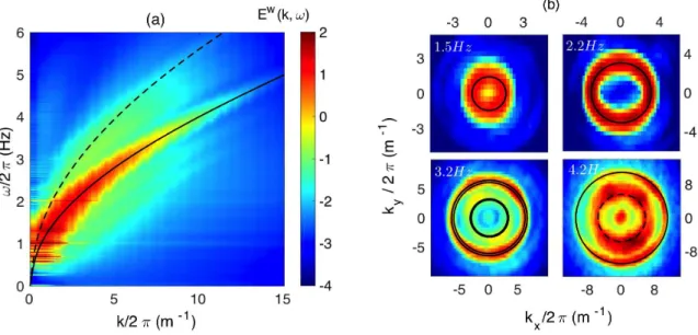
presented. We use the Stereo-PIV technique to measure the velocity of the water surface resolved in space and time. Figure 6 shows the full power spectrum of the vertical velocity Ew(k, ω) = h|w(k, ω)|2
i. Figure 6(a) shows the power spectrum Ew(k, ω) integrated over the direction of k. Energy is mainly concentrated along the linear dispersion
relation of deep water gravity waves ω = √gk (solid line). However for higher frequencies, a significant part of the energy lies away from the linear dispersion relation, in particular along the second harmonic ω =√2gk (dashed line). This point is clearly seen in Fig. 6(b) that shows cross-sections in the (kx, ky) plane of the full spectrum Ew(k, ω) at
four given frequencies 1.5, 2.2, 3.2 and 4.2 Hz. In addition to the observation of a quasi-isotropic system, we notice that at 4.2 Hz a major part of the energy is concentrated on the second harmonic which seems to indicate a strong level of non-linearities. This observation is potentially related to the limited spatial resolution of the measurement. As we study large values of ω, harmonic waves have a lower k than linear waves. At the highest frequencies, the size of the correlation box in the Stereo-PIV measurement does not allow us to measure linear waves, which amplitude is reduced by filtering, while harmonics remain observable because of their larger wavelengths at the same frequency. Space-time spectra were also observed recently in experiments[31, 32] by using arrays of local probes and the repeatability of the generation to construct a synthetic arrays with sufficient resolution. They observed also energy out of the dispersion
FIG. 6. (a) Space time Fourier power spectrum of the vertical velocity of the waves Ew(k, ω) for a typical experiment where the
mean wave steepness is ǫ = 0.11. The spectrum Ew(k, ω) has been integrated over directions of k. (b) Four cross sections of
the complete spectrum Ew(k, ω) at given frequencies (values indicated on the image). In both cases, the solid black line is the
deep water linear dispersion relation ω =√gk and the dashed line is its second harmonic. Energy is color-coded in log-scale.
relation with presence of harmonics. The excitation was rather narrowband and interpreted in the framework of the nonlinear Schr¨odinger equation.
a) -100 -50 0 x(cm) -60 -40 -20 0 20 y(cm) -3 -2 -1 0 1 2 3 uh.∇η(cm/s) 0 5 10 15 20 25 10−2 10−1 100 b) k/2π (m−1) C i, j C˙η,w C˙η,−u∇η C˙η,w−u∇η
FIG. 7. (a) Snapshot of uh· ∇η, the non-linear component of the vertical velocity field w = ∂η∂t + uh· ∇η. (b) Coherence of
the different components of the velocity relation (4) as a function of k. Assuming isotropy, the coherence is averaged over eight
directions of k regularly spread over a circle. The black curve is the coherence Cη,w˙ between the vertical geometric velocity ˙η
and w. The blue curve is the coherence Cη,−u˙ h·∇η
between ˙η and −uh.∇η. The red curve is the coherence C
˙
η,w−uh between
˙η and w − uh· ∇η (see (5) for definitions).
In order to perform a quantitative analysis of the strength of the non-linearities, we compute the non-linear term uh· ∇η in the the kinematic surface condition (a snapshot is shown in Fig. 7(a)) :
∂η
∂t = w − uh· ∇η (4)
between the different terms of equation (4) defined as:
Cη,w˙ (k) = |h ˙η∗(k,t)w(k,t)i|
q
h| ˙η|2ih|(w−u h·∇η)|2i
Cη,−u˙ h·∇η(k) = |h ˙η∗(k,t)(−uh·∇η)(k,t)i|
q
h| ˙η|2
ih|(w−uh·∇η)|2i
Cη,w−u˙ h·∇η(k) = |h ˙η∗(k,t)(w−uh·∇η)(k,t)i|
q
h| ˙η|2
ih|(w−uh·∇η)|2i
(5)
where the average h·i is an average over time and ˙η = ∂η∂t.
Using our choice of a common normalization of the coherence allows us to compare directly the three coherence esti-mators along the dimension k. The coherence Cη,w−u˙ h.∇η(red line) should be equal to one in a perfect measurement.
However, the inevitable presence of noise decreases this level at high k (where the signal over noise ratio is getting lower). We observe that the coherence fraction of the non-linear term increases with k up to a maximum around 10% before dropping due to the noise. The proximity of the black and red curve confirms the weakly-nonlinear character of our system which is thus expected to be in the range of validity of the WTT, as far as the strength of non-linearity is concerned.
IV. INVESTIGATION OF 3-WAVE INTERACTIONS
1. Theoretical analysis
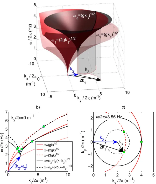
Both temporal and spatio-temporal observed power spectra are inconsistent with the predictions of the WTT possibly due to additional dissipation or finite size effects as discussed above. Yet, if the theory is applicable to our experiment, resonant interactions should exist and be the main mechanism to transfer energy. We start our analysis by investigating 3-waves interactions. Strictly resonant theoretical solutions can be found geometrically using the linear dispersion relation. Figure 8(a) shows the ensemble of solutions for a given pair (k2, ω2). As expected, the
dispersion relation of ω1 (in pink surface) does not intersect with the linear dispersion of ω2+ ω3 (black surface).
As it is well known for pure gravity waves, this means that no exact 3-waves solution exist for freely propagating waves following the linear dispersion relation. However, the analysis of the power spectrum showed that up to 10% of the energy lies in the second harmonic and some energy is scattered around the dispersion relation. In the following we consider the correlations between Fourier modes that may not follow the linear dispersion relation but that are resonant nonetheless, i.e. that follow the 3-wave resonance relations (1). Some of these modes are typically bound waves that result from the quadratic interaction of two free waves.
We start by including the second harmonic to look for resonant solutions as the red surface ω1=√2gk1in Fig. 8(a).
One observes the existence of an intersection with the black surface ω2+ ω3, suggesting the possibility of resonant
interactions involving waves that do not necessarily fulfill the linear dispersion relation. Figures 8(b) and (c) show two cross-sections of the Fig. 8(a) at given plans ky/2π = 0 m−1 and ω/2π = 3.56 Hz (resp.) for a better view of the
solutions (green dots). Among these solutions, one is the special case of a wave interacting with itself to form its own harmonic : k2= k3= k0 so that k2+ k3= k1= 2k0 (and similar equations for ω).
We also note that in vicinity of this bound wave solution, the two dispersion curves (black and red curves) remain very close to each other. This may allow quasi-resonant interactions :
k2+ k3= k1 ω2+ ω3= ω1+ δω (6)
where δω is the detuning that will allows resonance if the width ∆Ω of the power spectrum is larger (∆Ω > δω). From Fig. 6, it can be seen that ∆Ω varies significantly across the Fourier space but it takes typical values of order a few tenth of Hz while Fig. 8(b) shows that the distance between the continuous red and black curves remains extremely small across a wide interval around their intersection (at the center of the figure). From this observation we may expect quasi-resonant interactions over an interval of frequencies of width about 1 Hz. However, ∆Ω is far too small to generate resonant interactions between the two linear branches (pink and black line, separated by about 1 Hz), in contrast to what has been observed in gravity-capillary waves turbulence [22, 23].
The second harmonic ω1=√2gk1and the third harmonic ω1=√3gk1are also shown in Fig. 8(b) with the dashed
black line and the dashed red line respectively. They show similar features so that one could expect quasi-resonances in between second and third harmonics.
0
5
10
0
1
2
3
4
5
6
7
ω
/2
π
(Hz)
k
x/2
π
(m
1)
b)
ω=(gk)1/2 ω=(2gk)1/2 ω=(3gk)1/2 ω=ω 2+|g(k−k2)| 1/2 ω=ω 2+|2g(k−k2)| 1/2(k
2,
ω
2)
k
y/2
π
=0 m
−10
1
2
3
4
5
−2
−1
0
1
2
c)
k
y/2
π
(m
− 1)
k
x/2
π
(m
−1)
k
22k
1ω
/2
π
=3.56 Hz
k
3FIG. 8. (a) 3D Theoretical exact geometrical solution for 3-wave resonant interactions. For simplicity, only the positive
frequencies are represented. A first linear dispersion relation ω1(k1) is shown in light pink. We pick a value of the pair (k2, ω2)
shown with the blue arrow. We then plot a second linear dispersion relation in black starting from the point (k2, ω2). This
black surface is thus ω2+ ω3(k3= k − k2). Any intersection of both surfaces corresponds to resonance ω1= ω2+ ω3. As it is
well known, we observe no intersection between the pink and black curves, as no 3-wave resonances are geometrically allowed
for wave following the linear dispersion relation ω =√gk. The red surface is the second harmonic ω1=√2gk1. The intersection
of the red and the black surface indicates the presence of resonant solutions when the wave labeled 1 is a second harmonic of the linear dispersion relation and the waves 2 and 3 are linear waves. These are usually known as bound harmonics where
k2+ k3= 2k1. (b) Cross-section of the 3D representation for ky/2π = 0 m
−1
. The third harmonic ω =√3gk is added as the
red dashed line and the second harmonic ω3=
√
2gk3 is added as the black dashed line starting from the point (k2, ω2). Exact
solutions are indicated by the green dots. Note that in the vicinity of some solutions (large values of kx at the right of the
figure), the two dispersion relations remain close for a large range of frequencies, suggesting the possibility of quasi-resonance (see text). (c) Cross-section of (a) for a given frequency ω/2π = 3.56Hz. Exact solutions are plotted with green dots.
0
2
4
6
8
0
2
4
6
8
a)
ω
3/2
π
(Hz)
ω
1/2
π
(Hz)
ω
2/2
π
=2Hz
0
2
4
6
8
0
2
4
6
8
ω
3/2
π
(Hz)
ω
2/2
π
(Hz)
b)
−2.5
−2
−1.5
−1
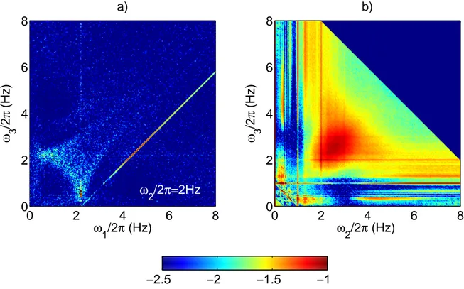
FIG. 9. a) Normalized third order correlation Cω
3(ω1, ω2, ω3) for a given wave ω2/2π = 2 Hz. A high concentration of correlations
is present along the resonant line ω1 = ω2+ ω3, suggesting the presence of 3-wave interactions. b) Bicoherence B3ω(ω2, ω3). A
red spot is visible around ω2= ω3= 2π × 2.5 Hz.
2. Correlations
3-wave resonant interactions are investigated using third order correlations. We start the analysis in frequency space using the third order correlation of the vertical velocity.
c3ω(ω1, ω2, ω3) = hw∗(ω1)w(ω2)w(ω3)i (7)
in order to check the presence of resonant frequency triads satisfying ω1= ω2+ ω3. Figure 9(a) shows this correlation
estimator for a given frequency ω2/2π = 2 Hz and normalized so that to ensure 0 ≤ Cω3 ≤ 1 [33]:
C3 ω(ω1, ω2, ω3) = c3 ω(ω1, ω2, ω3) r D |w(ω2)w(ω3)|2 E D |w(ω1)|2 E (8)
The resonant line ω1= ω2+ ω3is clearly observed above the statistical noise (which level is about 10−2.5) indicating
the presence of 3-wave resonances in the system. Figure 9(b) shows the bicoherence:
Bω3(ω2, ω3) = Cω3(ω2+ ω3, ω2, ω3) (9)
which corresponds to the extraction of the resonant line of C3
ω. A wide spot of strong correlations (about 25%) appears
when ω2&2.5 Hz and ω3&2.5 Hz as well. The high correlation values for similar values of ω2 and ω3 indicates that
coupling with harmonic waves may be present close to the bound waves solutions where ω2 is equal to ω3.
To obtain a more precise view of the coupling we have to extend the analysis in the wavenumber and frequency domain in order to distinguish the different branches (linear and harmonics). This can be done with the space and time bicoherence: B3 k,ω(k2, k3, ω2, ω3) = hw ∗(k 2, ω2)w(k3, ω3)w(k2+ k3, ω2+ ω3)i r D |w(k2, ω2)w(k3, ω3)|2 E D |w(k2+ k3, ω2+ ω3)|2 E (10)
The large dimensionality of parameter space imposes to choose the value of some components to be more easily understandable. To be in the same representation as the theoretical solution presented in Fig. 8, we impose a wave (k2, ω2) on the linear dispersion relation. In order to improve the statistical convergence, we average the bicoherence
over eight directions of the wavevector k2 (isotropically spread in direction). Figure 10 shows four cross-sections of
B3 k,ω for |k2| /2π = 4 m−1. 0 5 10 15 k 1x/2π (m -1) 0 1 2 3 4 5 6 7 8 9 ω /2 π (Hz) a) 0 5 10 15 k x 1/2π (m -1 ) -6 -4 -2 0 2 4 6 k y 1 /2 π (m -1 ) b) ω/2π = 4 Hz 0 5 10 15 k 1x/2π (m -1 ) -6 -4 -2 0 2 4 6 k 1 y /2 π (m -1 ) c) ω/2π = 5 Hz 0 5 10 15 k1x/2π (m-1) -6 -4 -2 0 2 4 6 k 1 y /2 π (m -1 ) d) ω/2π = 6 Hz
−2
−1.5
−1
−0.5
FIG. 10. 3D Bicoherence B3k,ω(k2, k3, ω2, ω3) for a given wave (k2, ω2) (with |k2|/2π = 4 m
−1
). In order to allow a direct
comparison, the axes are the same than those of figure 8 and show k1= k2+ k3 and ω1= ω2+ ω3. The x axis is given by the
direction of k2. The black arrows show the wave (k2, ω2). (a) Cross-section in the plane (kx, ky = 0, ω). The red and black
curves are similar to ones shown in fig 8. Exact resonances with harmonics are at the intersection of a black curve and a red one. A high correlation intensity is observed in these regions, suggesting the occurrence of interaction between linear waves and harmonics. (b), (c) and (d) are three cross-sections in the planes corresponding to given values of ω/2π = 4, 5 and 6 Hz.
An angular dispersion of the interactions of about 90◦
The cross-section corresponding to the unidirectional solutions (ky = 0) is plotted in Fig.10(a) in the same
repre-sentation as Fig. 8(b) . Solid and dotted lines are representing the linear dispersion relations and the second harmonic with the same colorcoding as in Fig.8. The correlation presents several areas of high intensity above 10%. Two of them are located near the exact bound waves solution. We note also that these high correlation regions show a strong spreading lying on the region where the two dispersion curves (linear and harmonic) remain close. This confirms the presence of quasi-resonant interactions in the system which are at the same order of magnitude than the exact bound solution. It is noticeable that the exact bound waves solution does not display any specificity as compared to the approximate resonances. As expected, there is no quasi-resonant interaction between the two linear branches because their separation is stronger than the spectrum width ∆k/2π ≈ 0.5 m−1.
Figures 10 (b), (c) and (d) show three cross-sections at a given frequencies. Again, we observe that high correlation regions are located near the intersections of black and red curves (exact resonances). As seen before in the case of the unidirectional cross-section, a spread of the high correlations is present due to quasi-resonant interactions. This leads to a uniform area of correlation that covers an angular distribution of about 90◦ around the direction of k
2. Some
other areas of high correlation can be seen, in particular for negative k3(solid black curve) or for negative frequencies
ω3(in Fig.10(a), correlations around (0 − 2) Hz). These results are puzzling since no exact or quasi-resonant solutions
can be found to explain their presence. Moreover, the Fourier component at (k1, ω1) has extremely weak energy in
the power spectrum. We suspect an effect of coupling due to partially standing waves. Indeed due to the finite size of the container all waves are not fully freely propagating waves. Part of the energy is due to standing waves made of the superposition of waves at several wavevectors (but the same frequency) that are phase matched. This could cause additional spurious resonances among seemingly non resonant waves. However no actual proof can be proposed at this time.
3. Field data from the Black Sea
k/2
π
(m
−1)
ω
/2
π
(Hz)
a)
0
1
2
0
0.5
1
1.5
2
−5
−4
−3
−2
−1
k x/2π (m −1 ) k y /2 π (m − 1 ) −1 0 1 −1 0 1E
η(k,
ω
)
1Hz
0
1
2
0
0.5
1
1.5
2
b)
k
x/2
π
(m
−1)
ω
/2
π
(Hz)
−2
−1.5
−1
−0.5
0
FIG. 11. (a) Power spectrum Eη(k, ω) of surface gravity waves measured by Leckler et al. [30] in the Black Sea. Inset,
cross-section of the complete spectrum at a given frequency of 1 Hz. The solid line is the linear dispersion relation and the
dashed line is the second harmonic. (b) Cross-section along k2, ω2(ky/2π = 0m
−
1) of the 3D bicoherence Bk,ω
3 (k2, k3, ω2, ω3)
for a given wave (k2, ω2) computed from the same dataset. The red and black curves are similar to ones shown in Fig. 8. Exact
solutions are in the region where the black curve intersects the red one. A high correlation intensity is observed at this region, suggesting the occurrence of quasi-resonant interaction between linear waves and harmonic.
Thanks to the dataset of in-situ stereoscopic measurements in the Black Sea by Leckler et al.[30], we are able to reproduce and compare the previous correlation analysis with actual sea waves. Surface gravity waves have been mea-sured using a stereoscopic measurement based on a direct cross-correlation of the sea using natural patterns generated by the surface roughness (ripples) and impurities under diffuse lightning. The measurement is performed over a field of about 15 × 20 m2during 30 minutes. This larger size allow by Nature is thus far enough to diminish strongly the
effects of surface pollution caused by Marangoni waves as discussed above. Figure 11 a) shows a reproduction of their measured power spectrum Eη(k, ω). Energy is present at frequencies ranging from 0.3 Hz to roughly 2 Hz. Like for
the experiment presented above, the energy is mainly distributed around the linear dispersion relation but a small fraction of the energy is on the second harmonic. The main difference is that waves are quite anisotropic (see inset that shows the spatial distribution of the energy at 1 Hz, showing that only negative kx are present) instead of an
isotropic system as in our experiment.
Figure 11(b) displays a cross-section of the 3D bicoherence similarly as Fig. 10(a) above at ky/2π = 0 m−1.
Although the estimator is less converged than for the experiment due to a smaller amount of data, we clearly observe the presence of a high correlation area in the proximity of the black and the red curve (exact solutions). Like for our experiment, no quasi-resonant interactions between the two linear branches (pink and black curves) can be seen. Finally, the main difference with the experiment is the absence of the unexplained correlations on the negative parts of (k2, ω2). This absence supports the suggestion of that they may be related to standing waves in our experiment
since these are not present in this field dataset.
V. 4-WAVE INTERACTIONS
0
2
4
6
8
0
2
4
6
8
a)
ω
4/2
π
(Hz)
ω
2/2
π
(Hz)
0
2
4
6
8
0
2
4
6
8
ω
4/2
π
(Hz)
ω
3/2
π
(Hz)
b)
ω
1/2
π
=2.2Hz
−2.5
−2
−1.5
−1
FIG. 12. (a) Normalized fourth order correlations Cω
4(ω1, ω2, ω3, ω4) for two given waves ω1/2π = 2.2 Hz and ω3/2π = 3.2 Hz
in the experiment. A very weak value of correlations is present on the resonant line ω1+ ω2 = ω3+ ω4 (dashed line) at the
highest frequencies (ω2/2π > 5 Hz). At low frequencies where linear waves exists, there is no evidence of 4-wave interactions at
the level of convergence which is about 10−2.5. (b) Tricoherence Bω
4(ω1, ω3, ω4). Like in (a), only a weak correlation is observed
at the highest frequencies. The light blue on the bottom left corner of the figure (ω3/2π < 2.2 Hz) is not statically converged.
The two red lines correspond to the trivial solution ω3= ω1 and ω4= ω2 (or ω4= ω1 and ω3= ω2).
The previous analysis shows that 3-wave coupling exists between linear and harmonic waves, both in the experiment and in the sea. We now investigate of 4-waves interactions that actually predicted to operate the turbulent cascade by the WTT. We compute the fourth order correlation in frequency normalized by the power spectrum.
Cω4(ω1, ω2, ω3, ω4) = hw ∗(ω 1)w∗(ω2)w(ω3)w(ω4)i r D |w(ω1)w(ω2)|2 E D |w(ω3)w(ω4)|2 E (11)
Figure 12 a) shows this estimator for two arbitrary given frequencies ω1/2π = 2.2 Hz and ω3/2π = 3.2 Hz at which a
the resonant line for this pair (ω1, ω3). A significant correlation area is emerging but only at the highest frequencies
(ω2/2π ≥ 5 Hz). Its origin is unclear and may be due to noise as the spectrum is very weak at these frequencies and
mostly at the noise level.
In order to test more resonant configurations beyond this given pair, we compute the tricoherence Tω4(ω1, ω3, ω4) = C4 ω(ω1, ω3+ ω4− ω1, ω3, ω4) r D |w(ω1)w(ω3+ ω4− ω1)|2 E D |w(ω3)w(ω4)|2 E (12)
We give one value of the frequency ω2to obtain 2D pictures. Figure 12(b) displays the tricoherence for ω1/2π = 2.2 Hz.
The two red lines are the trivial solutions corresponding to ω3 = ω1 and ω4 = ω2 (or ω4 = ω1 and ω3 = ω2) and
thus their value is not relevant. At low frequencies, where linear waves exists (with a significant level of energy in the spectrum), there is still no evidence of 4-waves interaction since the observed coherence values are very weak. They are most likely not converged and they remain close to the statistical background noise. This pattern has been check for other given values of the frequency and leads to the conclusion that no 4-waves correlations are observed at our convergence level for this experiment.
0
0.5
1
1.5
2
0
0.5
1
1.5
2
ω
2/2
π
(Hz)
a)
ω
4/2
π
(Hz)
ω
1/2
π
=0.6Hz
ω
3/2
π
=0.9Hz
0
0.5
1
1.5
2
0
0.5
1
1.5
2
b)
ω
4/2
π
(Hz)
ω
3/2
π
(Hz)
ω
1/2
π
=1Hz
−2.5
−2
−1.5
−1
FIG. 13. Normalized fourth order correlation Cω
4(ω1, ω2, ω3, ω4) computed for the in-situ dataset. Two arbitrary frequencies
are given ω1/2π = 2.2 Hz and ω3/2π = 3.2 Hz. A significant level of statistically converged correlation is present along the
resonant line ω1+ ω2 = ω3+ ω4 (dashed line). b) Tricoherence T4ω(ω1, ω3, ω4) for ω1/2π = 1 Hz. The two dark red lines
correspond to the trivial solution ω3= ω1and ω4= ω2 (or ω4= ω1and ω3= ω2). A significant level of correlation can be seen
out of these trivial lines.
We then repeat the same analysis for the Black Sea dataset. Figure 13 shows a sample of both the fourth oder correlation C4
ω and the tricoherence Tω4. Although the statistical convergence is not as good as in the experiment a
line of significant correlation levels shows up in Fig. 13(a), in contrast with what was observed in the experiment. The tricoherence (fig13 b)) displays a significant value in a large part of the frequency space. In particular there is no special accumulation close to the trivial point ω1= ω2= ω3= ω4 (intersection of the two red lines) which mean that
the wave coupling is not necessarily strongly local. We note some organization with lines, suggesting that a few modes are more effective (at 0.7 Hz or 1.4 Hz for instance). Due to the superposition of solutions in the frequency space, it is not possible to get more information from these plots. The next step is thus to do a space and time analysis like for the 3-wave analysis. Unfortunately the number of realizations that permits to converge a statistical estimator decreases strongly in a full (k, ω) domain due to the impossibility to perform spatial averaging. Thus, it does not
permit to converge significantly the space and time tricoherence for which the correlation level is weaker than the one observed in the 3-wave analysis.
VI. DISCUSSION AND CONCLUDING REMARKS
The correlation analysis that we presented confirms the presence of resonant interactions among pure gravity surface waves. However, the first results do not correspond to the theoretical expectations of 4-wave interactions. Although no 3-wave interactions are observed between linear waves as predicted by the theory, we actually observe 3-wave coupling between the linear component and harmonic. These kinds of coupling are usually known as bound waves where a wave interacts with itself to form its own harmonic. However the resonances are not restricted to strict harmonics and we observe also quasi-resonant interactions that appear to be very active as well. These new solutions enhance the potential efficiency of these interactions among all possible bound waves. The remaining question is the contribution of the 3-waves coupling in the generation of the global energy cascade. Indeed, despite strong correlations, the energy of the harmonic branch remains low (maximum of 10%). A bound wave resulting from the quadratic interaction of free waves, 3-wave interaction involving a bound wave can appear as a 4-free-wave interaction. This is actually the meaning of the normal-form reduction which is performed in the application of the weak turbulence theory [5, 34]. The observed resonant coupling involving the second harmonics and near resonant bound waves maybe a privileged route for the global 4-wave process.
0 200 400 600 800 1000 −4 −2 0 2 4 6 Time (s) log10(E η (ω ,t)) ω/2π=1Hz τ=484s τω/2π=484 ω/2π=2Hz τ=770s τω/2π=1540 ω/2π=3Hz τ=450s τω/2π=1350 ω/2π=4Hz τ=390s τω/2π=1560
FIG. 14. Time evolution of the power spectrum Eη(ω, t) for four frequencies 1, 2, 3and4 Hz. An exponential decrease is observed
(dashed lines) and leads to a typical time scale τ following e−t
τ. We assume that the dissipative timescale Tdis Td≈ τ .
Surprisingly, the 4th order correlation analysis in our experiment does not show traces of 4-waves interactions that are supposedly at the core of the energy transfers for surface gravity waves. A turbulent-like spectrum is observed that suggests that an energy cascade is operating nonetheless. Two hypotheses may be proposed. The first one is that our convergence level remains too low to permit the observation of a possible very weak level of 4-waves correlations. The second hypothesis is that the dissipation is too strong and breaks the scale separation that is the core of the theory. The typical 4−wave non-linear time scale of energy transfers for this experiment, can be roughly estimated as TN L
4w = ǫ2(4−2)1
2π
ω ≈ 7000 2π
ω [2]. It may become larger than the typical time scale for the dissipation
Td. The latter decreases strongly with the presence of Marangoni waves and it has been estimated by studying the decrease of the energy when the forcing is stopped. Figure 14 shows this evolution for four given frequencies. We observe an exponential decrease e−tτ that permits to define the dissipation time as Td ≈ τ. We found an order of
magnitude Td ≈ 10002π
ω for the range of our measured waves. The prediction for the 3-waves nonlinear time scale
gives TN L 3w = ǫ2(3−2)1 2π ω ≈ 80 2π ω. Thus we have TL< TN L 3w < Td< T4wN L (13)
and this supports the situation where only 3-waves interactions are observed. From this observation, we may propose that the additional dissipation does not permit the usual waves resonant interactions and the cascade may thus be
generated through 3-waves interactions using the harmonic branch.
Since the scales are much larger in the ocean, the field measurements are less affected by the additional dissipation by the Marangoni waves. We then expect to observe classical wave turbulence through only 4-waves interaction for weak enough waves if TN L
4w < Td. Indeed, the 4-waves correlations show a signature of 4-waves interactions for the
Black Sea dataset. The mean level of these interaction remain lower (about 5%) than the 3-waves interactions with the harmonic branch (about 25%) that are also observed in this regime. However, due to the weak energy level of the harmonic branch, it is possible that a significant part of the transfer occurs through these 4-waves interactions. This observation is in agreement with the exponent of the power spectrum which is close to the theoretical prediction while keeping a very weak non-linearity with ǫp = 0.02 as seen in Fig. 5. Nevertheless it should be noted that although
the wave steepness is much lower in the Black Sea than in the experiment (by roughly one order of magnitude) the harmonic branch remains very visible in the spectrum and the 3-wave correlations level remains quite high. This observation suggests that, for a finite level of nonlinearity, the 3-wave resonant coupling with the harmonic that we describe here may actually be an important mechanism for the energy redistribution even when 4-wave coupling is operating.
To sum up, 4-waves interactions seem to exist but their very low occurrence probability and their associated long time scale make them very sensitive to the presence of dissipation in the inertial range. This is especially the case of very weakly non-linear regimes where the non-linear interaction time become very high. Our observations suggest an additional, faster and thus more efficient 3-wave coupling mechanism for the energy transfers. The question is whether these 3-wave interactions can play a role in the turbulence cascade and replace the weak turbulence 4-waves process.
ACKNOWLEDGMENTS
This project has received funding from the European Research Council (ERC) under the European Union’s Hori-zon 2020 research and innovation programme (grant agreement No 647018-WATU). A.C. and the project were also supported by Fondation Simone et Cino Del Duca and Institut de France.
[1] V. E. Zakharov, V. S. L’vov, and G. Falkovich, Kolmogorov Spectra of Turbulence (Springer, Berlin, 1992). [2] S. Nazarenko, Wave Turbulence (Springer, Berlin, 2011).
[3] A. C. Newell and B. Rumpf, “Wave turbulence,” Ann. Rev. Fluid Mech. 43 (2011).
[4] VE Zakharov, “Kolmogorov spectra in weak turbulence problems,” in Basic Plasma Physics: Selected Chapters, Handbook
of Plasma Physics, Volume 1 (1984) p. 3.
[5] K. Hasselmann, “On the non-linear energy transfer in gravity-wave spectrum. part 1. general theory,” J. Fluid Mech. 12, 481–500 (1962).
[6] Michael Berhanu and Eric Falcon, “Space-time-resolved capillary wave turbulence,” Phys. Rev. E 87, 033003 (2013). [7] Eric Falcon, Claude Laroche, and S. Fauve, “Observation of gravity-capillary wave turbulence,” Phys. Rev. Lett. 98,
094503 (2007).
[8] Eric Falcon, U. Bortolozzo, and S. Fauve, “Capillary wave turbulence on a spherical fluid surface in low gravity,” EPL (Europhysics Letters) 86, 14002 (2009).
[9] Luc Deike, Daniel Fuster, Michael Berhanu, and Eric Falcon, “Direct numerical simulations of capillary wave turbulence,” Phys. Rev. Lett. 112, 234501 (2014), 1406.0795.
[10] P. Cobelli, A. Przadka, P. Petitjeans, G. Lagubeau, V. Pagneux, and A. Maurel, “Different regimes for water wave turbulence,” Phys. Rev. Lett. 107, 214503 (2011).
[11] Sergey Nazarenko, S. Lukaschuk, Stuart McLelland, and Petr Denissenko, “Statistics of surface gravity wave turbulence in the space and time domains,” J. Fluid Mech. 642, 395 (2009).
[12] Luc Deike, B Miquel, T Jamin, B Semin, Michael Berhanu, Eric Falcon, and F Bonnefoy, “Role of the basin boundary conditions in gravity wave turbulence,” J. Fluid Mech. 781, 196—-225 (2015).
[13] Petr Denissenko, S. Lukaschuk, and Sergey Nazarenko, “Gravity wave turbulence in a laboratory flume,” Phys. Rev. Lett.
99, 014501 (2007).
[14] Elena Kartashova, “Wave resonances in systems with discrete spectra,” Am. Math. Soc. Trans. , 95–130 (1998).
[15] A Pushkarev, “On the kolmogorov and frozen turbulence in numerical simulation of capillary waves,” Eur. J. Mech., B/Fluids 18, 345–351 (1999).
[16] Sergey Nazarenko, “Sandpile behaviour in discrete water-wave turbulence,” J. Stat. Mech.: Theory and Experiment 02002, 1–8 (2013), 0510054 [nlin].
[17] B. Miquel, A. Alexakis, and N. Mordant, “Role of dissipation in flexural wave turbulence: from experimental spectrum to kolmogorov-zakharov spectrum,” Phys. Rev. E 89, 062925 (2014).
[18] T. Humbert, O. Cadot, G. D¨uring, C. Josserand, S. Rica, and C. Touz´e, “Wave turbulence in vibrating plates : the effect of damping,” EPL 102, 30002 (2013).
[19] Werner Alpers and Heinrich H¨uhnerfuss, “The damping of ocean waves by surface films: A new look at an old problem,”
J. Geophys. Res. 94, 6251 (1989).
[20] F Behroozi, Kimberly Cordray, and William Griffin, “The calming effect of oil on water,” Am. J. Phys. 75, 407 (2007). [21] A. Przadka, B. Cabane, V. Pagneux, A. Maurel, and P. Petitjeans, “Fourier transform profilometry for water waves: how
to achieve clean water attenuation with diffusive reflection at the water surface?” Exp. Fluids 52, 519–527 (2011). [22] Quentin Aubourg and N. Mordant, “Nonlocal resonances in weak turbulence of gravity-capillary waves,” Phys. Rev. Lett.
114, 1–5 (2015).
[23] Quentin Aubourg and Nicolas Mordant, “Investigation of resonances in gravity-capillary wave turbulence,” Phys. Rev. Fluids 1, 023701 (2016), 1605.04091.
[24] Quentin Aubourg, Etude exp´erimentale de la turbulence d’ondes `a la surface d’un fluide. La th´eorie de la Turbulence Faible
`
a l’´epreuve de la r´ealit´e pour les ondes de capillarit´e et gravit´e, Ph.D. thesis, Universit´e Grenoble Alpes (2016).
[25] Peter A. Kralchevsky and Kuniaki Nagayama, “Capillary interactions between particles bound to interfaces, liquid films and biomembranes,” Adv. Colloid Interface Science 85, 145–192 (2000).
[26] W. A. Gifford and L. E. Scriven, “On the attraction of floating particles,” Chemical Engineering Science 26, 287–297 (1971).
[27] M. Aziz Tayfun, “Narrow-band nonlinear sea waves,” J. Geophys. Res. : Oceans 85, 1548–1552 (1980).
[28] Herv´e Socquet-Juglard, Kristian B. Dysthe, Karsten Trulsen, Harald E. Krogstad, and Jingdong Liu, “Probability distri-butions of surface gravity waves during spectral changes,” J. Fluid Mech. 542, 195–216 (2005).
[29] M. Onorato, L. Cavaleri, S. Fouques, O. Gramstad, Peter A.E.M. Janssen, J. Monbaliu, A. R. Osborne, C. Pakozdi, M. Serio, C. T. Stansberg, a. Toffoli, and K. Trulsen, “Statistical properties of mechanically generated surface gravity waves: a laboratory experiment in a three-dimensional wave basin,” J. Fluid Mech. 627, 235 (2009).
[30] Fabien Leckler, Fabrice Ardhuin, Charles Peureux, Alvise Benetazzo, Filippo Bergamasco, and Vladimir Dulov, “Analysis and Interpretation of Frequency-Wavenumber Spectra of Young Wind Waves,” J. Phys. Ocean. 45, 2484—-2496 (2015). [31] Tore Magnus A Taklo, Karsten Trulsen, Odin Gramstad, Harald E Krogstad, and Atle Jensen, “Measurement of the
dispersion relation for random surface gravity waves,” Journal Of Fluid Mechanics 766, 326–336 (2015).
[32] Tore Magnus A Taklo, Karsten Trulsen, Harald E Krogstad, and Jos´e Carlos Nieto Borge, “On dispersion of directional surface gravity waves,” Journal Of Fluid Mechanics 812, 681–697 (2017).
[33] W.B. Collis, P.R. White, and J.K. Hammond, “Higher-order spectra: the bispectrum and trispectrum,” Mechanical
Systems and Signal Processing 12, 375–394 (1998).
[34] Krasitskii V, “On reduced equations in the Hamiltonian theory of weakly nonlinear surface waves,” Journal Of Fluid Mechanics 272, 1–20 (1994).