HAL Id: hal-01522009
https://hal.archives-ouvertes.fr/hal-01522009
Submitted on 12 May 2017
HAL is a multi-disciplinary open access
archive for the deposit and dissemination of
sci-entific research documents, whether they are
pub-lished or not. The documents may come from
teaching and research institutions in France or
abroad, or from public or private research centers.
L’archive ouverte pluridisciplinaire HAL, est
destinée au dépôt et à la diffusion de documents
scientifiques de niveau recherche, publiés ou non,
émanant des établissements d’enseignement et de
recherche français ou étrangers, des laboratoires
publics ou privés.
Time Shifting in LiDAR Bathymetric Waveforms
Anis Bouhdaoui, Jean-Stéphane Bailly, Nicolas Baghdadi, Lydia Abady
To cite this version:
Anis Bouhdaoui, Jean-Stéphane Bailly, Nicolas Baghdadi, Lydia Abady. Modeling the Water Bottom
Geometry Effect on Peak Time Shifting in LiDAR Bathymetric Waveforms. IEEE Geoscience and
Remote Sensing Letters, IEEE - Institute of Electrical and Electronics Engineers, 2014, 11 (7),
pp.1285-1289. �10.1109/LGRS.2013.2292814�. �hal-01522009�
F
Modeling the Water Bottom Geometry Effect on Peak
Time Shifting in LiDAR Bathymetric Waveforms
Anis Bouhdaoui, Jean-Stéphane Bailly, Nicolas Baghdadi, and Lydia Abady
Abstract—Bathymetry is usually determined using the positions
of the water surface and the water bottom peaks of the green LiDAR waveform. The water bottom peak characteristics are known to be sensitive to the bottom slope, which induces pulse stretching. However, the effects of a more complex bottom ge- ometry within the footprint below semitransparent media are less understood. In this letter, the effects of the water bottom geometry on the shifting of the bottom peaks in the waveforms were modeled. For the sake of simplicity, the bottom geometry is modeled as a 1D sequence of successive contiguous segments with various slopes. The positions of the peaks in waveforms were deduced using a conventional peak detection process on simulated waveforms. The waveforms were simulated using the existing Wa-LID waveform simulator, which was extended in this study to account for a 1D complex bottom geometry. An experimental design using various water depths, bottom slopes, and LiDAR footprint sizes according to the design of satellite sensors was used for the waveform simulation. Power laws that explained the peak time shifting as a function of the footprint size and the water bottom slope were approximated. Peak shifting induces a bias in the bathymetry estimates that is based on a peak detection of up to 92% of the true water depth. This bias may also explain the frequent underestimation of the water depth from bathymetric airborne LiDAR surveys observed in various empirical studies.
Index Terms—Altimetry, laser noise, laser radar, sea floor.
I. INTRODUCTION
ULL-waveform LiDAR is a technology that registers the backscattered laser pulse power over time, i.e., along the laser beam path, as it penetrates successive media. In many environmental applications, the peaks in the waveforms are the basic information used to retrieve useful variables and parameters, such as elevations or media thickness values (e.g., water depth and forest height) [1]. In a remote opaque media, such as bare soil or building materials, it has been demonstrated that the target geometry within the footprint highly modifies the waveforms [2], particularly if the footprint is wide. Numerous analytical equations relating the waveform properties to the slope within the footprint exist in the literature [2], [3]. The main known impact of laser target geometry, i.e., the incidence angle, is the effect of pulse stretching. In bathymetric LiDAR,
because of the semitransparent nature of the medium (water) that is penetrated by the laser beam before reaching the bottom, the physics differs from those of topographic LiDAR. However, the effects of the water bottom geometry on the waveforms also show a stretching effect [3], [4]. Some analytical formulations were proposed to explain pulse stretching as a function of the target slope [4]–[6]. Empirical studies on the accuracy of LiDAR airborne bathymetry [7], [8] often report observed biases, i.e., a systematic underestimation of the bathymetry estimates. However, explanations on the physical causes of these biases are few and vary among studies, most likely because of the lack of highly detailed reference data on the target properties at the airborne footprint scale that can help researchers better understand these causes.
Assuming a Gaussian spatial distribution of laser pulse en- ergy within the laser beam solid angle (beam profile) [9], we hypothesize that this underestimation originates from the bot- tom peak position in waveforms that may be highly disturbed due to the water bottom geometry. In this letter, we aimed at qualitatively and quantitatively testing this hypothesis using an existing bathymetric LiDAR waveform simulator.
For that purpose, a specific 1D water bottom geometry model was included in the Wa-LID simulator for this study. An intensive experimental design was used to analyze and assess the bottom geometry effects on the bathymetry’s accuracy. This analysis was performed according to the wide LiDAR footprints that are expected in future LiDAR bathymetric satellite sensors. This letter first presents the methods, including 1) the ap- proach used to model the water bottom geometry within a given footprint and 2) the detailed protocol with which the Wa-LID simulator was used to account for the water bottom geometry. Furthermore, a qualitative analysis of the simulated waveform under controlled conditions was conducted. Finally, we modeled the relationships between the time shifting of the waveform peaks and the bottom slope, the water depth, and the footprint size for a steepened segment geometry.
II. METHODS
The bathymetry of coastal waters, i.e., the water depth, is a key parameter for hydrodynamics engineering, navigation, and aquatic environments. Its value to areal supports, such as the LiDAR footprint, can be directly deduced from the water bottom geometry within this support if the water sur- face is flat. To further investigate the link between the water bottom geometry and the accuracy of bathymetry estimates from LiDAR waveforms, we first proposed a simplified 1D geometric model of the water bottom. Indeed, we assumed that the 1D bottom geometry model, despite being a simplification, is appropriate for demonstrating the impact of the bottom geometry on water depth estimation. We then demonstrated
1
Thus, the mean water depth Z¯ of a given LiDAR footprint can be defined as the weighted average of all mean water depths
Z¯i of segment Si , i.e., n−1 Z¯ = L Z¯ n−1 with L = L . (5) L i i i=1 i i=1
If we substitute Z¯i from (4) into (5), the bathymetry Z¯ could
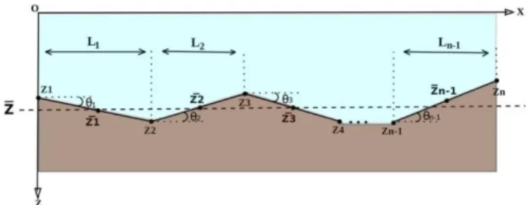
be written as Fig. 1. Simplified 1D water bottom geometry along the footprint diameter
(X -axis). The z-axis denotes the water depth. Z = 0 is the water surface. n−1 2
Z¯ = Z + 1 Li
n−1 i−1
how to use an existing bathymetric waveform simulator using this modeled geometry. Finally, we presented an experimental
1
L i=1 2 tan(θi ) +
i=2 k=1
Li (Lk tan(θk )) .
(6) design for waveform simulation to investigate the water bottom
geometry effect on the peak time shifting in LiDAR waveforms. However, to highlight only the effect of the bottom geometry, additional sources of perturbations in actual data from LiDAR systems were neglected in the simulation, including the beam wander, scintillation, and shape distorsion of emitted pulses and capillary wave effects.
A. Linking Bathymetry to the Water Bottom Geometry Properties at the Footprint Scale
For a given LiDAR footprint of diameter F p, we modeled the water bottom geometry as a 1D series of n − 1 contiguous segments that are denoted Si for i ∈ (1, . . . , n − 1) having n
endpoints denoted Zj with j ∈ (1, . . . , n). Each segment Si is
defined by its length Li , which corresponds to its projection on
the abscissae axis and a slope angle θi with respect to this same
abscissae axis (see Fig. 1). The water depths at the endpoints of segment Si are denoted Zi and Zi+1 .
Z¯i corresponds to the mean water depth of each segment Si ,
and Z¯ is the bathymetry at the footprint scale, i.e., the mean water depth throughout the LiDAR footprint. Knowing Z1 and the segment parameter pairs (θi , Li ) allows for the calculation
of the mean water depth, i.e., bathymetry Z¯, as illustrated below.
First, using a descending Cartesian Z-axis and the properties of geometric series, the water depth of endpoint Zj of segment Si is j−1 ∀j ∈ (2, . . . , n) Zj = Z1 + Lk . tan(θk ). (1) k=1
By definition, the mean water depth Z¯i of segment Si is thus
Using the proposed water bottom geometric model and knowing the bathymetry at footprint size Z¯, all segment pairs (θi , Li ), Z1 and any segment endpoint Zi or segment mean
water depth Z¯i can be computed. It is also possible to compute
the water depth for any position x along the X abscissae axis.
B. Waveform Simulation
To simulate LiDAR waveforms using a modeled water bottom geometry, we assume that the mean water depth Z¯, the angles (θi )i∈(1,...,n−1) , and the length of each segment
(Li )i∈(1,...,n−1) are given. Because the water bottom is a finite
continuous medium and an analytical model of a waveform cannot be simply defined with this bottom geometry, we chose to develop a discretization approach.
In this approach, the series of segments describing the water bottom geometry is spatially sampled along the X -axis into
m samples (x1 , . . . , xf , . . . , xm ) with the spatial lag Δx . At
a given sample xf along the X -axis with a water depth of Zf ,
a waveform denoted Pbf (t) with a footprint diameter of F p
and a null slope angle is simulated using the Wa-LID simulator [10], where the water bottom is assumed to be a Lambertian reflector [11]. We assumed that illuminating a nonflat bottom can be approached by illuminating a staircase function with the Δx spatial lag, i.e., a mix of flat bottoms of the same size F p but with different water depths Zf for f ∈ (1, . . . , m). In
this approach, the slope of the water bottom at the Δx scale is
neglected.
Consequently, the resulting simulated waveform at the foot- print scale, considering the complex water bottom geometry, is computed by averaging the waveforms Pbf (t) and accounting
for the Gaussian beam profile, i.e.,
m ∀i ∈ (2, . . . , n − 1) Z¯ i = Zi + Zi+1 . (2) 2 Pb (t) = f =1 wf ∗ Pbf (t) (7)
Substituting Zi and Zi+1 from (1) into (2), we obtain
where wf is the weight corresponding to a Gaussian beam
profile, i.e., i−1 Lk . tan(θk ) + i Lk . tan(θk ) 1 (xf − 0.5Fp )2 Z¯i = Z1 + k=1 k=1 2 . (3) wf = σ 2π√ exp 2σ2 (8)
Extending this computation for each i ∈ (2, . . . , n − 1) gives with σ = Fp /6 (∼99.7%). i−1 Z¯i = Z1 + Lk . tan(θk ) + k=1 where Z¯1 = Z1 + L1 /2. tan(θ1 ). L i . tan(θ ) (4) 2 i
In practice, the waveform simulator 1) identifies the starting sample of the discretization; 2) defines the next m, i.e., the number of required samples, which depends on Δx and F p;
3) calculates the depth for each sample position f ; 4) simulates and stores the Pbf (t) waveform of a flat bottom at depth Zf ;
p
and 5) simulates the average waveform from the discretization process.
To avoid discretization disturbance in the simulations and based on the Nyquist–Shanon sampling theorem, sampling interval Δx must be smaller than half of the time sampling
resolution in the LiDAR digitizer, i.e., 1 Δx ≤
2 cw Tp (9) where cw = 225563 km.s−1 is the speed of light in water,
and T p is the LiDAR time sampling lag corresponding to the inverse of the digitizing rate (typically of 1 GHz). Here, Δx = 0.1125 m was used.
C. Waveform Peak Detection
Many heuristics exist to retrieve the bathymetry Z¯ from a LiDAR waveform. A basic approach is to identify the surface and bottom positions in the waveforms using a multi-Gaussian fitting of the peaks. This is an effective approach in the case of an actual signal with noise. In the waveform simulation process, we chose to turn off the noise addition because the objective of this study was not to test an inversion method but only to analyze the effect of the bottom geometry on the accuracy of the bathymetry estimates. We thus chose to use a simple waveform peak detection method instead of a multi-Gaussian fitting. This method assumes that a peak is the highest point between valleys, i.e., a local maximum; thus, the algorithm used searches for local maxima.
The first peak is usually assumed to be the water surface po- sition, and the latest peak is assumed to be the bottom position. The bathymetry can thus be deduced simply by transforming the time difference into distance.
D. Experimental Design
LiDAR waveform simulations were performed using the configuration of a satellite LiDAR sensor illuminating a semi- transparent coastal water. In the simulations, the usual green Nd:Yag laser wavelength (532 nm) was used, as has been used in many Airborne LiDARs [12]. This wavelength is used to obtain a tradeoff between the attenuation of the bottom return due to water absorption and scattering by particles in the water. The sensor parameters were fixed and chosen to agree with the configurations studied by the EADS-Astrium company (European Aeronautic Defence and Space Company) [13], particularly regarding laser energy. Because the limit of expo-sure to laser radiation (LLR) is 5.10 −3 J/m2 for wavelengths between 400 and 700 nm (including the green laser with a 532-nm wavelength) [14], [15], the maximum allowed energy E0 (J) by the LiDAR that meets the standards of ocular safety is defined as
πF
2 LLR
TABLE I
WATER PARAMETERS USED . BOT TO M PARAMETERS A RE IN BOLD
TABLE II
SPECIFI CATION OF SENSOR PARAMETERS
which is linked to the sensor elevation (meters) and the LiDAR divergence angle (rad) through the following equation:
Fp = H. tan(γ). (11)
From (9) and (10), the values of E0 and γ can be calculated because all other parameters are fixed.
Based on a previous review [13], the water parameter values were fixed and chosen to be representative of clear coastal waters with reflective bottoms [13], [16], [17]. The chosen sensor and water parameters are all listed in Tables I and II.
Waveform simulations were performed for the following mean water depths Z¯ at the footprint scale: 2, 5, 8, and 12 m. Five different footprint sizes F p were also used: 5, 10, 20, 30,
and 40 m. The slope segment angle was varied between 0◦ and 50◦, with a step size of 1◦. The waveforms resulting from these different configurations were used to quantify and model the effect of the bottom geometry on the bathymetry estimates. For the sake of simplicity, a geometry with a single steep segment was used.
III. RESULTS AND DISCUSSION
A. Qualitative Analysis of the Simulated Waveforms
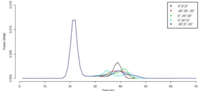
To highlight the influence of the bottom geometry on the shape of the LiDAR waveforms, Fig. 2 shows five waveforms using different configurations of slope angles of three succes- sive segments of equal length that describe the geometry of
E0 ≤
4TatmMscintMgauss
(10)
G2 the water bottom. For all waveforms, a mean water depth Z¯ (bathymetry) of 2 m and a LiDAR footprint F p of 5 m were where Tatm = 0.5 is the atmospheric transmittance; Mscint =
2 is the margin for atmospheric scintillation; Mgauss = 4.6 is the margin for Gaussian beam (factor overload in the center of a Gaussian); G = 13.34 is the binocular magnification used by the observer in the ground; Fp is the LiDAR footprint size,
used.
Fig. 2 shows that the bottom peaks for complex water bottom geometries can be shifted to the left or right of the bottom peak of the flat-bottom configuration (0◦/0◦/0◦). This finding signi-fies that a complex bottom geometry can produce bottom peaks
Fig. 2. LiDAR waveforms for five water bottom geometries. In each LiDAR footprint F p(= 5 m), the bottom geometry is composed of three segments. The configuration of the bottom slope angles of successive segments (θ1 , θ2 , θ3 ) are: (0◦/0◦/0◦), (−30◦/30◦/ −30◦ ), (0◦/−30◦/30◦ ), (0◦/30◦/0◦ ),
and (−30◦/0◦/−30◦ ). 1 ns is equivalent to 11.25 cm.
Fig. 3. Influence of the water bottom slope on the LiDAR waveform. F p = 5 m, Z¯ = 2 m, one segment with θ = [0◦ , 5◦ , 10◦ , 15◦ , 20◦ , 25◦ , 30◦ ]. Here, 1 ns is equivalent to 11.25 cm.
that can induce an over- or underestimation of the water depths. For instance, the bottom geometry configuration (0◦/30◦/0◦) depicted in dark gray produces a waveform that contains one peak for the water surface and two peaks for the water bottom contribution, with a last bottom peak located at a water depth of 2.47 m. The other cases show stretched peaks after the water surface peak with a delay from the true bottom position in the waveform abscissae axis ranging from approximately −7 to 4.2 ns, corresponding to a deviation of about −0.79 to 0.47 m in the water depth estimation. These schematic examples confirm that it is not accurate to estimate the water depth only from the latest peak position if the water bottom geometry is complex.
B. Quantitative Peak Shifting Analysis
From the previous examples, we chose to analyze in detail the effect of the bottom geometry on the peak time shifting using only one segment with a bottom slope θ and the experi- mental design of water depths and footprint sizes F p described in the previous section. Fig. 3 shows the resulting waveforms for F p equal to 5 m, Z¯ equal to 2 m, and θ ranging from 0◦ to 30◦ with a step size of 5◦.
First, the water bottom peak approaches the water surface peak when the water bottom slope increases. This shifting of the bottom peak may result in an underestimation of the water depth. For example, for a footprint of 5 m and Z¯ = 2 m, the water depth is underestimated by 0.089 m at a slope of 10◦
Fig. 4. Underestimation of bathymetry at the footprint scale as a function of the water bottom slope.
tends to expand with a lower amplitude when the bottom slope increases. This stretching effect may also participate in bottom peak time shifting.
This bottom peak shift is explained by the strongest contri- bution to the waveform coming from the shallowest part of the bottom section due to the semitransparency of water. In fact, the bottom peaks resulting from the shallowest samples have higher amplitudes due to lower attenuation. The stretching of the bottom peak when the water bottom slope increases is due to the discretized convolution between the emitted pulse and either a decrease or increase in the bottom depth when the slope is not zero [7].
The bottom peak time shifting in the waveform leads to a bias in the estimation of bathymetry. An analysis of this bias according to the water bottom slope angle revealed a power function relationship. Fig. 4 illustrates the error in the bathymetry estimates for two different LiDAR footprints with a steep water bottom: small footprint F p = 5 m and large footprint F p = 40 m.
Fig. 4 shows that for a mean water depth of 2 m and a LiDAR footprint F p of 5 m, the highest investigated bottom slope θ is 32◦. Higher slope angles make the segment modeling the water bottom go out of the water. For a footprint F p of 40 m and a mean water depth of 2 m, the highest investigated bottom slope
θ is 4◦ (see Fig. 4).
Fig. 4 also demonstrates that the underestimation of the mean water depth highly depends on both the LiDAR footprint F p and the bottom slope θ but only slightly depends on the mean water depths for the four tested depths Z¯ = (2, 5, 8, 12) m. We can model this underestimation with a generalized power law for given F p and Z¯ values, i.e.,
ΔZ = a|θ|b . (12)
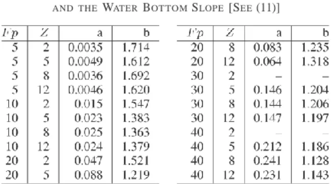
For each F p and Z¯, Table III shows the value of the (a, b) coefficients that were estimated from a nonlinear fitting process of the power law [see (11)], which yielded high R2 values (close to 99.6%). As shown in Table III, the values of a increase as F p increases, whereas the values of b decrease toward 1 as
F p increases. In addition, coefficient a varies with the mean
water depth only for high F p (a slight increase is observed). For low F p values, coefficient a appears to be independent of the mean water depth.
We then performed multiple linear regressions between the a or b coefficients of (11) and parameters F p and Z¯, i.e., and by 1.213 m at a slope of 30◦. It is apparent that the return
pulse broadening is also observed. In fact, the bottom peak
a = α1 F p + β1 Z¯ + γ1
b = α2 F p + β2 Z¯ + γ2 .
TABLE III
a AND b COEFFI CIENTS OF THE RELATIONSHIP BETWEEN THE
UNDERESTIM AT ION O F T HE MEAN WATER DEPTH AND THE WATER BOT TO M SLOPE [SEE (11)]
The underestimation of the mean water depth described in (11) can then be written as
Z¯+γ )
increases with an increase in the LiDAR footprint and bottom slope. For a mean water depth of 2 m and F p = 5 m, the bathymetry underestimation is approximately 0.0235 m for
θ = 4◦ and 0.651 m for θ = 20◦. For the same water depth and F p = 40 m, the underestimation is approximately 1.10 m for θ = 4◦. The bias of the water depth estimates was further modeled as a generalized power law of the LiDAR footprint size, bottom slope, and water depth.
These results show that the bathymetry from the LiDAR waveform for a rough water bottom at the footprint scale should not be based only on the peaks in the waveform. These conclu- sions are valid when any laser beam penetrates semitransparent media before reaching the bottom and could be applicable for other laser wavelengths in other contexts. However, more formulations for other complex water bottom geometries with more contiguous segments or facets within the footprint should
also be investigated in future works.
ΔZ = (α1 F p + β1 Z¯ + γ1 )θ(α2 F p+β2 2 (14)
REFERENCES
where α1 = 0.0044, β1 = 0.0001, γ1 = −0.0043, α2 = 0.0001, β2 = −0.0002, γ2 = 1.2399, and R2 = 99.6%.
It is apparent that this final formulation is only valid for the sensor and water configurations explored, with the exception of a footprint size F p related to the height of the sensor and a simple bottom geometry corresponding to a steep plane. It is also only valid for the Gaussian beam profile. If the footprint is pixelated, i.e., divided into subfootprints with smaller F p, the biases originating from the water bottom geometry are reduced accordingly. Finally, the formulation that we proposed must be considered a particular situation of these bathymetry biases that is available for clear waters and highly reflective bottoms. In the event of more turbid waters and less reflective bottoms, the biases may be higher. However, the bottom geometry effect is a source of bathymetry bias. Other sources of bias exist due to laser pointing noise [18], Gaussian emitted pulse shape deformation [1], and wave slope variability at the surface [17].
IV. CONCLUSIO N
The information required to retrieve the bathymetry from a green LiDAR waveform is the detection of the positions of the surface and bottom peaks in the waveform. The bottom peak (position and intensity) is dependent on the water bottom morphology, i.e., geometry, within the footprint. A 1D model assimilating the bottom geometry to a series of segments of varying length and slope was developed and integrated into the existing Wa-LID code to simulate bathymetric LiDAR wave- forms for any footprint size and water depth. The effect of the water bottom slope on the water depth estimates was analyzed using water bottom configurations with only one steep segment. The results show a significant decrease in the delay in the waveform between the water surface and the bottom peaks when the water bottom slope increases. This decreasing delay is due to a shift in the bottom contribution due to a higher contribution of the laser backscattered energy from the top of the bottom slopes within the footprint. If the positions of the peaks in the waveform are used to retrieve bathymetry, this shift leads to a systematic underestimation, i.e., a bias in the bathymetry measurement, which depends mainly on the LiDAR footprint, the water bottom slope, and slightly on the water depth. This underestimation of the water depth obviously
[1] C. Mallet and F. Bretar, “Full-waveform topographic lidar: State-of-the- art,” ISPRS J. Photogramm. Remote Sens., vol. 64, no. 1, pp. 1–16, Jan. 2009.
[2] B. Jutzi and U. Stilla, “Range determination with waveform recording laser systems using a Wiener filter,” ISPRS J. Photogramm. Remote Sens., vol. 61, no. 2, pp. 95–107, Nov. 2006.
[3] Z. Liu, R. Li, X. Xi, L. Tang, and C. Li, “Modeling and simulation return waveforms from forest canopy of large footprint lidar,” in Proc. SPIE, 2009, pp. 74981L-7–74981L-8.
[4] R. E. Walker and J. W. McLean, “Lidar equations for turbid media with pulse stretching,” Appl. Opt., vol. 38, no. 12, pp. 2384–2397, Apr. 1999. [5] O. K. Steinvall and K. R. Koppari, “Depth sounding lidar: An overview of
Swedish activities and future prospects,” in Proc. SPIE, 1996, pp. 2–25. [6] C.-K. Wang and W. D. Philpot, “Using airborne bathymetric lidar to detect
bottom type variation in shallow waters,” Remote Sens. Environ., vol. 106, no. 1, pp. 123–135, Jan. 2007.
[7] G. C. Guenther, A. G. Cunningham, P. E. LaRocque, and D. J. Reid, “Meeting the accuracy challenge in airborne lidar bathymetry,” in Proc.
EARSeL-SIG-Workshop LIDAR, 2000, pp. 1–27.
[8] J. Bailly, Y. LeCoarer, P. Languille, C. Stigermark, and T. Allouis, “Geostatistical estimation of bathymetric lidar errors on rivers,” Earth
Surf. Process. Landforms, vol. 35, no. 10, pp. 1199–1210, Aug. 2010.
[9] P. Schaer, J. Skaloud, S. Landtwing, and K. Legat, “Accuracy estimation for laser point cloud including scanning geometry,” presented at the 5th International Symposium Mobile Mapping Technology, Padova, Italy, May 29–31, 2007.
[10] H. Abdallah, N. Baghdadi, J. Bailly, Y. Pastol, and F. Fabre, “Wa-LiD: A lidar waveform simulator for waters,” IEEE Geosci. Remote Sens. Lett., vol. 9, no. 4, pp. 744–748, Jul. 2012.
[11] H. M. Tulldahl and K. O. Steinvall, “Analytical waveform generation from small objects in lidar bathymetry,” Appl. Opt., vol. 38, no. 6, pp. 1021– 1039, Feb. 1999.
[12] A. Axelsson, “Rapid topographic and bathymetric reconnaissance using airborne lidar,” in Proc. Soc. Photo-Opt. Instrum. Eng., 2010, vol. 7835, pp. 783 503-1–783 503-10.
[13] H. Abdallah, J. Bailly, N. Baghdadi, N. Saint-Geours, and F. Fabre, “Po- tential of space-borne lidar sensors for global bathymetry in coastal and inland waters,” IEEE J. Sel. Topics Appl. Earth Observ. Remote Sens., vol. 6, no. 1, pp. 202–216, Feb. 2013.
[14] “Guidelines on limits of exposure to broad-band incoherent optical radia- tion (0, 38 to 3 micrometre),” Health Phys., vol. 73, pp. 539–554, 1997. [15] “Revision of guide-lines on limits of exposure to laser radiation of wave-
lengths between 400 nm and 1.4 micrometre,” Health Phys., vol. 79, pp. 431–440, 2000.
[16] G. H. Tuell and J. Y. Park, “Use of shoals bottom reflectance images to constrain the inversion of a hyperspectral radiative transfer model,” in
Proc. SPIE, Laser Radar Technol. Appl. IX, Sep. 13, 2004, vol. 5412,
pp. 185–193.
[17] H. M. Tulldahl and S. A. Wikstrom, “Classification of aquatic macrovege- tation and substrates with airborne lidar,” Remote Sens. Environ., vol. 121, pp. 347–357, Jun. 2012.
[18] T. Urban, B. Schutz, and A. Neuenschwander, “A survey of ICES at coastal altimetry applications: Continental coast, open ocean island, and inland river,” Terr. Atmos. Ocean. Sci., vol. 19, no. 1/2, pp. 1–19, Apr. 2008.