HAL Id: hal-03103443
https://hal.archives-ouvertes.fr/hal-03103443
Submitted on 8 Jan 2021
HAL is a multi-disciplinary open access
archive for the deposit and dissemination of
sci-entific research documents, whether they are
pub-lished or not. The documents may come from
teaching and research institutions in France or
abroad, or from public or private research centers.
L’archive ouverte pluridisciplinaire HAL, est
destinée au dépôt et à la diffusion de documents
scientifiques de niveau recherche, publiés ou non,
émanant des établissements d’enseignement et de
recherche français ou étrangers, des laboratoires
publics ou privés.
Distributed under a Creative Commons Attribution - NonCommercial| 4.0 International
License
Reference Field (IGRF-13)
I. Wardinski, Diana Saturnino, Hagay Amit, A. Chambodut, Benoit Langlais,
M. Mandea, E. Thebault
To cite this version:
I. Wardinski, Diana Saturnino, Hagay Amit, A. Chambodut, Benoit Langlais, et al.. Geomagnetic
core field models and secular variation forecasts for the 13th International Geomagnetic Reference
Field (IGRF-13). Earth Planets and Space, Springer/Terra Scientific Publishing Company, 2020, 72
(1), �10.1186/s40623-020-01254-7�. �hal-03103443�
FULL PAPER
Geomagnetic core field models and secular
variation forecasts for the 13th International
Geomagnetic Reference Field (IGRF-13)
I. Wardinski
1*, D. Saturnino
2, H. Amit
2, A. Chambodut
1, B. Langlais
2, M. Mandea
3and E. Thébault
4Abstract
Observations of the geomagnetic field taken at Earth’s surface and at satellite altitude are combined to construct continuous models of the geomagnetic field and its secular variation from 1957 to 2020. From these parent models, we derive candidate main field models for the epochs 2015 and 2020 to the 13th generation of the International Geomagnetic Reference Field (IGRF). The secular variation candidate model for the period 2020–2025 is derived from a forecast of the secular variation in 2022.5, which results from a multi-variate singular spectrum analysis of the secular variation from 1957 to 2020.
Keywords: The geomagnetic field, Geomagnetic secular variation, Geomagnetic field models, Forecasts of the geomagnetic field
© The Author(s) 2020. This article is licensed under a Creative Commons Attribution 4.0 International License, which permits use, sharing, adaptation, distribution and reproduction in any medium or format, as long as you give appropriate credit to the original author(s) and the source, provide a link to the Creative Commons licence, and indicate if changes were made. The images or other third party material in this article are included in the article’s Creative Commons licence, unless indicated otherwise in a credit line to the material. If material is not included in the article’s Creative Commons licence and your intended use is not permitted by statutory regulation or exceeds the permitted use, you will need to obtain permission directly from the copyright holder. To view a copy of this licence, visit http://creat iveco mmons .org/licen ses/by/4.0/.
Introduction
The International Association of Geomagnetism and Aeronomy (IAGA) regularly releases the International Geomagnetic Reference Field (IGRF), which is a math-ematical description of Earth’s main magnetic field and its secular variation. Previous versions (e.g., Finlay et al.
2010; Thébault et al. 2015) are widely used in many
dis-ciplines of Earth sciences and applied for navigational
purposes (Jiménez et al. 2012; Canciani and Raquet 2016)
and in satellite orientation (Slavinskis et al. 2014).
In this study, we combine geomagnetic field observa-tions taken at Earth’s surface and at satellite altitude to construct continuous models of the geomagnetic core field and its secular variation between 1957 and 2020. From these models, candidate models for the IGRF
(Alken et al. 2020), i.e., main field models for the epochs
2015 and 2020 and a secular variation model for the period 2020 to 2025 centered at 2022.5 are derived. We apply two modeling techniques to derive these models.
First, a method that descends from the time-dependent modeling technique developed by Bloxham and Jackson
(1992); we refer to this as the classical model. The second
technique is based on a method for constructing core field models that satisfy the frozen-flux radial magnetic induction equation on the core-mantle boundary (CMB) by imposing the field evolution to be entirely due to advection of the magnetic field at the core surface (Lesur
et al. 2010; Wardinski and Lesur 2012), which we refer to
as the kinematic field model. The latter method could be understood as a simple data assimilation approach, where the diffusion-less induction equation and assumptions about the dynamical regime of the core flow form the pri-ors, and observations define their likelihood.
Methods of forecasting the future geomagnetic field evolution range from simple linear extrapolation to data assimilation into numerical dynamo simulations (Kuang
et al. 2010; Aubert 2015; Fournier et al. 2015). Here, we
devise two strategies to forecast the geomagnetic secular variation. First, a direct forecast based on a multi-variate singular spectrum analysis (MSSA) (Broomhead and
King 1986; Plaut and Vautard 1994) of the magnetic field
variability of past decades. Second, a kinematic forecast scheme is applied that is also based on the MSSA, but
Open Access
*Correspondence: wardinski@unistra.fr
1 Institut de Physique du Globe de Strasbourg, Université de Strasbourg/
EOST, CNRS, UMR 7516, Strasbourg, France
of the core flow variability of past decades. The recon-struction of the past flow variability and its forecast are used to predict the future geomagnetic field by forward-modeling the diffusion-less radial induction equation on the CMB. This approach is somewhat similar to geo-magnetic field forecasts using steady and time invariant
flows (Beggan and Whaler 2010; Hamilton et al. 2015;
Whaler and Beggan 2015). However, such forecasts are
expected to fail at the occurrence of geomagnetic jerks that are sudden changes in the secular variation. Such
events occurred in the past decades (Mandea et al. 2010;
Brown et al. 2013), most recently in 2014 (Torta et al.
2015). The cause of these events is not fully understood.
Their occurrences have been related to different types of rapid wave motion within Earth’s liquid core (Bloxham
et al. 2002; Aubert and Finlay 2019), temporal changes of
the core flow (Wardinski et al. 2008) and Earth’s rotation
variation (Holme and de Viron 2005, 2013).
This paper is organized as follows. “Geomagnetic field
modeling” section outlines the two techniques to derive the parent geomagnetic field model for the IGRF candi-dates. In the third section, we develop the methodology
to predict future geomagnetic secular variation. “Results
and discussion” section provides results of the geomag-netic field modeling, secular variation forecasts and the derivation of the candidate models. The last section dis-cusses the results and concludes the study.
Geomagnetic field modeling
In this section, we summarize the derivation of a parent geomagnetic main field model from which we deduce an
IGRF candidate model. The parent model, hereafter C3FM3,
covers the period from 1957 to 2020. The model derivation
follows that of Wardinski and Lesur (2012) and consists of
two branches, a classical model without the kinematic
con-straint applied (see “Classical modeling” section), and a
kin-ematic field model based on the tangential geostrophic flow
assumption (see “Kinematic field modeling” section). Like
in the previous model, C3FM2, we use order 6 B-splines to
parameterize field and flow coefficients in time. The spline knot spacing is set to be roughly 1.5 years. Both model branches are constrained to fit a main field model for the epoch 2015. This main field model is based on magnetic measurements taken by the Swarm satellite mission (Lesur, priv. comm.). We choose 2015, as it is the epoch of the last IGRF, with a good data coverage provided by geomagnetic observatories and the Swarm satellite mission. This data coverage decreases towards the model endpoint.
Data
In this work, we use two types of data, measurements taken at a network of ground-based geomagnetic obser-vatories and satellite data taken at satellite virtual
geomagnetic observatories (Mandea and Olsen 2006).
The idea of combining ground-based and virtual observa-tory data to perform a geomagnetic field modeling was
already carried out by Barrois et al. (2018). However, here
we derive secular variation estimates to avoid leakage of sub-annual external field variations into the description of the core field and to obtain a sufficient representation of the short-term secular variation, that may be used to forecast geomagnetic field changes.
Ground‑based geomagnetic observatories
A large portion of the data used in this study comes from ground-based observatories. Like in previous studies
(War-dinski and Holme 2006; Wardinski and Lesur 2012; Lesur
et al. 2018), we derive estimates of secular variation by
annual differences from observatory monthly means, where these monthly means are averages of observatory hourly means. Also, annual means are used for observatories for which hourly mean values are not available from the World
Data Centre for Geomagnetism - Edinburgh (2019). These
observatory annual means are part of a compilation that is provided by the British Geological Survey - Edinburgh
(2020). Over the period 1957–2018 the number of
geomag-netic observatories simultaneously in operation that have been providing vectorial hourly means of North, East and downward components ranges between 72 and 155. Data errors were removed when encountered and data gaps were
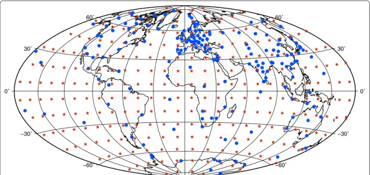
not filled by interpolations. Figure 1 maps locations of the
ground-based geomagnetic observatories used in this study.
Satellite virtual geomagnetic observatories
We use vector magnetic field measurements from Swarm Level-1b data product, version 0505 (0506 for some data files). All three Swarm satellites are considered for the period between January 2014 to June 2019. Data is screened for quality flags defined in the Level-1b Prod-uct Definition Document (Tøffner-Clausen and Nielsen
2018). We keep only measurements identified as
nomi-nal, and also Swarm C vector measurements after 4th November 2014.
We select only data where the Sun is below the
hori-zon (Chambodut et al. 2002). Additionally, we retain only
data showing moderate magnetic activity. Sectorial
mag-netic activity index a σ (Chambodut et al. 2013), provided
by the International Service of Geomagnetic indices
(2020), were used and we only select data corresponding
to a σ < 25 nT.
With the selected data we then construct a global mesh of virtual geomagnetic observatories (VO)
fol-lowing Saturnino et al. (2018), with some small
changes. An approximately equal area mesh is obtained with the VO centers separated in
θvo= ±6.40◦,±19.20◦,±32.0◦, . . . ,±83.20◦. In each
band, the longitude φvo of each VO and the number of
longitudinal divisions, NφVO (rounded up to the nearest
integer), are chosen so that:
The resulting mesh contains 258 VOs. Figure 1 displays
the locations of all VOs in the mesh. The data set of each VO consists of selected data acquired inside a cylinder
of 3.0◦ radius centered around each VO and during a
30-day period, i.e., leading to nearly monthly values. The Equivalent Source Dipole (ESD) technique is then used,
following closely Saturnino et al. (2018). For each month
(30-day period) the ESD inversion is applied to each VO vector data for the equivalent magnetization of dipoles placed at 2900 km depth inside Earth’s interior, by a least squares fit in an iterative, conjugate gradient, inversion
scheme (Purucker et al. 1996). Then, the forward
calcula-tion is used to estimate a magnetic field value at the VO center location and for a given time period. In this way, time series of magnetic field values at the center of each VO and at a constant altitude of 500 km, are obtained.
The distributions of ground-based and virtual
obser-vatories differ as can be seen in Fig. 1. Overall,
geomag-netic observatory locations cluster, which may lead to a higher spatial resolution of the model in some parts of the world, whereas in other parts the resolution may be lower than that of the virtual observatories.
(1)
Nϑvo =
360
12.8cos θvo.
Secular variation estimates
We derive secular variation estimates as input for the geomagnetic field modeling. The technique is applied to monthly means of VOs and to ground-based geo-magnetic monthly means. The secular variation of the
X-component at a given observatory is estimated as
where τ denotes a particular month. These are annual dif-ferences of observatory monthly means. Likewise, obser-vatory annual means are treated using
where t is in calendar years and dt is 1 year. Then,
secu-lar variation estimates derived by (2) and (3) are given in
nT/year.
Classical modeling
Conventional geomagnetic field modeling approaches rely on the assumption that Earth’s magnetic field
B(r, θ , φ, t) is a potential field without magnetic sources
in the mantle and in the vicinity of satellite virtual obser-vatories. Because of this, the geomagnetic field is deter-mined as a gradient of a scalar potential, i.e.,
(2) dX/dt|τ = X(τ + 6) − X(τ − 6) /dt, (3) dX/dt|t+1/2= X(t + 1) − X(t) /dt, (4) B(r, θ , φ, t)= −∇V (r, θ, φ, t) . −60˚ −60˚ −30˚ −30˚ 0˚ 0˚ 30˚ 30˚ 60˚ 60˚
Fig. 1 The distribution of ground-based and satellite virtual geomagnetic observatories. The ground-based observatory data (blue circles) cover the period 1957 to 2018, whereas the VO data (red stars) are derived from Swarm and cover the period 2015 to 2019.5
Then in a spherical geometry, the scalar potential of the geomagnetic field can be represented as
where a is Earth’s radius (6371.2 km), (r, θ, φ) the geo-centric spherical radial, co-latitude and longitude
coor-dinates and Pm
l (cos θ ) are the Schmidt quasi–normalized
associated Legendre functions, with their normalization defined by
with degree l and order m. The maximum spherical
har-monic degree in (5) is chosen to be lmax= 14 , to
mini-mize the contamination by the crustal field. The Gauss
coefficients {gm
l , hml } are expanded in time using order six
B-splines Mn(t):
The objective function �(m) to be minimized in the inversion is:
where A is an operator which relates the model vector m containing the Gauss coefficients to the data y . y − Am is the misfit between data and model, subject to the
regu-larization. Ce and Cm are the error and the prior model
covariance matrix, respectively. Cm is an expression of
the model priors.
Here, we report solutions that are adjusted to minimize
the integral of B2
r over the core surface to obtain a spatial
smooth model:
The matrix S has the diagonal elements
Like in some previous studies (Lesur et al. 2010;
War-dinski and Lesur 2012), we seek a reliable estimate of
the secular acceleration. Therefore, the temporal model
(5) V (r, θ , φ, t) = a lmax l=1 l m=0 (glm(t) cos(mφ) +hml (t) sin(mφ)) a r l+1 Plm(cos θ ) , (6) 2π φ=0 π θ=0
(Pml (cos θ ) cos(mφ))2sin θ dθ dφ= 4π
2l+ 1, (7) glm(t)= N n=1 glmnMn(t), hml (t)= N n=1 hmnl Mn(t). (8) �(m)= (y − Am)TC−1e (y − Am) + C−1m + C−1F , (9) S(c) B2r d�= mTS−1m. (10) sll, tll = (l+ 1) 2 2l+ 1 a c (2l+4) for l= 1 . . . , lmax.
constraint is to minimize the integral of the third time derivative of the radial field component over the core
sur-face and in the model period between tS and tE
where S(c) is the spherical surface of the core at radius
c= 3485 km . The diagonal elements of the matrix T are
the same as for S , and the time integral is computed using a Newton–Cotes formula of a closed type, e.g., Bode’s
rule (Abramowitz and Stegun 1973). Minimization of the
third time derivative requires placing further conditions on the second time derivatives of the radial field at the model end-points; best results are obtained when these are set to zero.
The model prior covariance matrix Cm is then given by:
The last term of (8) is the constraint to fit a given satellite
field in 2015, which is
where 0gm
l and 0hml are the Gauss coefficients of the
sat-ellite geomagnetic main field model. This constraint is necessary, as our model is based on secular variation data and it needs a main field model at a given epoch in order to provide also description of the main field at all times. Traditionally, we use a main field model that is derived in an independent study from satellite data. The constraint is then written
with the damping parameter f.
Solutions are sought iteratively in a very similar
man-ner as for the previous model, C3FM2, by deriving an
initial model to re-weight the observatory data by their residuals to this initial model. Then, the strength of exter-nal field variation is reduced by a noise-removal scheme
(Wardinski and Holme 2011). From this data set the final
model is derived.
Kinematic field modeling
In this section, we describe our method to invert geo-magnetic observations for field and flow at the core sur-face, which extends our previous study (Wardinski and
(11) 4π (tE− tS) tE tS S(c) ∂3B r ∂t3 2 d� dt = mTT−1m, (12) C−1m = SmTS−1m+ TmTT−1m. (13) F:= r=a (B−0B)2dS|t=2015 = lmax l=1 l m=0 (l+ 1)[(glm−0glm)2+ (hml −0hml )2]t=2015, (14) C−1F = fmTF−1m,
Lesur 2012), where we imposed the core flow to be purely toroidal. The inversion of secular variation data for field and flow at the core surface formulates to a Bayesian inference. Assuming a Gaussian distribution, then this
leads to an objective function similar to (8) that is
mini-mal for the preferred solution m.
In the following, we provide details of the prior infor-mation (constraints) used to derive a preferred solution of the non-unique and non-linear inverse problem. The constraints are applied on the portion of the model vec-tor that represents the core surface flow.
Here, we use the data set with the reduced external field
noise obtained in “Classical modeling” section to jointly
invert for the field and flow at the core surface. This eases the joint-inversion process, as it avoids the iterative solv-ing scheme to re-weight the data for the non-linear prob-lem. Different assumptions of the flow dynamic could
be applied (Holme 2007). Among them: purely toroidal
(Whaler 1980), tangential geostrophic (LeMouël 1984)
and quasi-geostrophic flow (Pais and Jault 2008).
How-ever, we focus on the tangential geostrophic flow assump-tion, as it is more comprehensive than a purely toroidal flow, but less restrictive than a quasi-geostrophic flow. (Note that the term flow refers to its horizontal part only, as the radial part vanishes at the core surface).
The flow is decomposed into toroidal and poloidal components:
T and P are scalars which are expanded in
Schmidt-nor-malized real spherical harmonics in space and B-splines
of order 6 in time, represented by tm
l (n), sml (n).
Following Lesur et al. (2010), the objective function of
the joint inversion for the field and the flow at the core surface reads
where the model vector m now contains the sets of Gauss
and flow coefficients. The functional 1 is related to the
kinematic constraint and defined by
˙
�(t) is a design matrix based on the radial induction
equation in the kinematic assumption, i.e.,
According to (18), the secular variation of the radial field
component at the core surface, ∂tBr , can be expressed in
terms of a core field, Br , advected by the core fluid flow,
u , where ∇h is the horizontal divergence. Then
(15) u= utor+ upol= ∇h× (ˆrT ) + ∇hP . (16) �(m)= (y − Am)TC−1e (y − Am) + 1�1(m), (17) �1(m)= t (Ag(t)· u − ˙�(t)· g)TCg(Ag· u − ˙�(t)· g) . (18) ∂tBr = −∇h· (uBr).
where g is a vector that contains the Gauss coefficients and u contains the flow coefficients. The elements of the
diagonal weight matrix Cg are defined as wg
l = 4π(l+1)2
(2l+1) .
Minimizing the mean square difference, integrated over the core surface S(c) and time, between the observed sec-ular variation and the secsec-ular variation generated by the
flow, then the functional 1 is equivalent to the integral
and we can write this (similarly to (9) and (11)) as
where m is now the model vector that holds the flow and Gauss coefficients. The diagonal elements of the field part
of K are given by Cg . The parameter
1 controls the
con-formity of the model to the kinematic constraint.
Because Ag(t) in the functional 1 depends on the
Gauss coefficients gm
l (t), hml (t) and is multiplied by u ,
this optimization problem (inversion) is clearly non-linear and has to be solved iteratively. However, the iterative process is unlikely to converge unless some constraints are applied on the flow model, as finding a flow model is an ill-posed inverse problem (Holme
2007). In order to obtain the optimal field model and
simultaneously reduce the null space for the flow, two types of constraints are considered. The flow model is forced to have a convergent spectrum, i.e., to be large scale, and to minimize Bloxham’s “strong norm”
(Blox-ham 1988; Jackson 1997),
N has the diagonal elements (l3(l+ 1)3)/(2l+ 1) . The
damping parameter S controls to what extent the flow
follows this constraint. Minimizing (21) constrains
effi-ciently the secular variation. Secondly the flow model is chosen such that it varies smoothly in time,
with T as the associated control parameter of the flow
temporal evolution that efficiently regularizes the inverse
problem. The constraints (21) and (22) are similar to
the temporal constraint of the classical model, i.e., (11),
as they involve a temporal integration to be minimized. Finally, it is required that the flow acceleration at starting and ending epochs is minimized by
(19) ˙ �(t)· g = Ag· u , (20) T S(c) ∂tBr(t)+ ∇h· (uBr) 2d� dt= gTK−1g, (21) T S(c) ∇h (∇h· u) 2 + ∇h(ˆr × ∇h· u) 2 d� dt= uTN u . (22) T S(c) (u)2d� dt = uTVu ,
t1 and t2 are the epochs 1957 and 2020.0, respectively.
This becomes necessary, as, if the flow acceleration is un-constrained at the endpoint, it may exceed realistic
val-ues. The factor E controls this constraint.
These are the basic settings for the joint inversion for the magnetic core field and the core flow. We impose a further constraint, in order to derive models that are based on different dynamical assumptions of the flow. One possible assumption commonly used is a tangential
geostrophic flow (Hills 1979; LeMouël 1984) which is
established by minimizing
where θ is the co-latitude. Elements of G are given by Pais
et al. (2004). The constraint is controlled by setting TG.
We apply two measures to discriminate models: the rms secular variation misfit is measured by differences between model and the observed secular variation, i.e.,
where Nobs is the number of observations. In addition,
for the kinematic field models we derive the ratio
that specifies to what extent the frozen-flux radial induc-tion equainduc-tion is satisfied. Values similar to 1 and larger mean that this constraint is not fulfilled by the model, and conversely values significantly smaller than 1 indicate that the frozen-flux radial induction equation is approxi-mately satisfied.
Forecasting schemes
In this study, we aim to obtain a description of (a) the temporal dynamics of the secular variation and (b) the temporal variability of the advective motion within the liquid outer core. These should not differ largely, but remaining external signals in the secular variation esti-mates may pose problems to identify clearly signals from the core. To forecast states of the physical system that lead to the secular variation it is necessary to analyze the observed time series. Our strategy relies on the deriva-tion of multi-variate time-series models, where individual secular variation and flow coefficients are treated as time series. (23) S(c) ∂u ∂t 2 d� t1,t2 = uTEu . (24) S(c) ∇h· (u cos θ)) 2d� = uTGu , (25) M = 1 (Nobs− 1) Nobs i=1 (Obs− Mod)2 (26) R(t) = S(c) ∂tBr(t)+ ∇h· (uBr) 2d� S(c) ∂tBr(t) 2 d�
Our development of time-series models and forecasts is based on the multi-variate singular spectrum analysis
(MSSA) (Broomhead and King 1986; Plaut and Vautard
1994, and see “Appendix A” section) of field and core flow
variability. Other methods could be chosen to find a suf-ficient description of the field and flow variability, such as ARIMA-models, or vector auto-regressions models; however, these model types are based on assumptions like stationarity of the time series and normality of the
residuals (Box and Jenkins 1976; Brockwell and Davis
2002, and references therein), which are unlikely for
the temporal variability of the geomagnetic field (Hulot
et al. 2010). Furthermore, the singular spectrum analysis
does not rely on assumptions about the linearity or non-linearity of the process that is generating the time series, whereas auto-regression models implicitly assume a lin-ear behavior of the observed data. If 1, . . . , T serves as the time range for a training set, then the model param-eters are estimated from these observations. The (out-of-sample) prediction is generated over the time range
T+ 1, . . . , T + h according to the generation mechanism
of the model. In this study we consider 10 years as the time range of the prediction. This sets h = 120 months. Prediction models are derived using the first 22 eigen-modes obtained by the MSSA of the temporal flow
vari-ability (see “Appendix A” section).
Direct secular variation forecast
The time series of the Gauss coefficients are taken from
the classical model branch of C3FM3. The analysis
con-siders discrete series of secular variation coefficients consisting in N observations regularly sampled in time.
The sampling time τs is chosen to be one month.
Time-series models are derived using a multi-variate singular spectrum analysis, where the temporal variabil-ity of the series is decomposed in eigenmodes (Vautard
et al. 1992; Golyandina et al. 2001; Ghil et al. 2002). The
time-series models are then reconstructions based on superposition of these eigenmodes, and similarly fore-casts. For the technical details of the model selection, we
refer the reader to “Appendix A” section.
Kinematic secular variation forecast
The kinematic forecasting scheme to predict future secular variation is motivated by results that the observed secular variation can be mostly explained by the advection of
mag-netic field (Roberts and Scott 1965; Wardinski and Lesur
2012). Additionally, results of a previous kinematic field
model show that the spatial complexity imposed by a satel-lite magnetic field model of 2004 is maintained backward
in time over decades (Wardinski and Lesur 2012). Here, we
(27)
want to explore to what extent the approach can be used to forecast geomagnetic field changes.
The scheme consists of two steps. First, we derive time-series models that give a sufficient accurate description of the temporal variability of the fluid motion in the liquid outer core. Therefore, we consider toroidal and poloi-dal flow terms, which are treated as discrete multi-variate time series from which we derive time-series models for a given ’learning’ phase. The learning phase is set to cover the interval 1957 to 2020.
The second step, the kinematic forecasting step, employs forward computation of the secular variation by using the diffusion-less induction equation and is initialized by
where ˜u(t0) represents the flow ( tlm(n), pml (n) ), and Br(t0)
the radial magnetic field at an initial epoch t0 . Here, we
use the flow coefficients of the kinematic branch of C3
FM3. The forecasts of ˜u(ti) for i = 0 are obtained by
deriving forecasts of the flow coefficients from their
time-series models, similar to the operation in “Direct secular
variation forecastDirect secular variation forecast” sec-tion. Generally, the forecasts of the secular variation are computed by
where δt represents the sampling interval of 1 month, and
˜u(tn) is the flow forecast vector that contains forecasts of
the individual flow coefficients for the first month after
2020.0. Equation (28) is computed on a spherical grid,
and then transformed to spherical harmonic secular
vari-ation coefficients ( ˙gm
l , ˙hml ) similar to the scheme of Lloyd
and Gubbins (1990). The forecast period is 120 months,
and ends in 2030.0.
Assessing the accuracy of forecasts
Choosing an appropriate error measure in forecasting is problematic, because no single measure gives an unam-biguous indication of forecasting performance, while the use of multiple measures makes comparisons between forecasting methods difficult and unwieldy (Mathews and
Diamantopoulos 1994). We apply a derivative of the widely
used mean absolute percentage error, i.e., the symmetric absolute percentage error (sAPE) to assess the difference between the observation, i.e., the actual field and flow coef-ficient y(t) and its forecast ˆy(t) as:
This follows the definition by Chen and Yang (2004),
which differs from those of Armstrong (1985), Flores
(28) ∂tBr(t1)= −∇h· ( ˜u(t0)Br(t0)), (29) ∂tBr(tn)= −∇h· ( ˜u(tn)Br(tn)), Br(tn+1)= Br(tn)+ ∂tBr(tn) δt, (30)
sAPE(t)= 2|y(t) − ˆy(t)|
|y(t)| + |ˆy(t)| .
(1986), as it does not become singular and has a
maxi-mum value of two when either y(t) or ˆy(t) is zero, but is
undefined when both are zero. The range of (30) is (0, 2),
i.e., the maximum value corresponds to 200% percent-age error. We define a prediction length, for which the
sAPE(t) becomes larger than 10%. This is a rather
cau-tious definition and other limits could also be considered.
Another measure that is widely used (e.g., Aubert 2015;
Whaler and Beggan 2015) is the rms-difference between
models
where Agm
l ,Ahml and Bglm,Bhml are Gauss coefficients of
the compared field models A and B. √dP represents
the total (difference) field integrated over the surface of the Earth, and similarly is the secular variation. We com-pute it in order to allow comparisons to other studies which use this measures as primary diagnostic. However,
we must note, that √dP is biased towards large-scale
contributions, when computed at Earth’s surface where the spatial energy spectrum of the field is decreasing, and is biased towards small scales at the core surface, where the spectrum is increasing. This is not the case for the
sAPE(t) , as it is relative to the amplitude of the actual
coefficient.
Results and discussion
In this section, we present results of the core field mode-ling and the secular variation forecasts. At the end of this section, we also present and discuss our candidates for the definitive geomagnetic reference field model (DGRF) in 2015, and IGRF candidate model for 2020.
We focus on two models: Model 1 was derived with the classical modeling approach and Model 2 is a kin-ematic field model based on the tangential geostrophic
flow assumption. Table 1 compiles the set of model
parameters and related model characteristics. Both mod-els provide almost equal fits to the data in terms of their residual standard deviation.
We note that, by strongly imposing the tangential geos-trophic constraint, the fit to the radial induction equation deteriorates, when compared to solutions with a weaker
tangential geostrophic constraint, see Appendix Table 3.
The reason for this is not clear, but, perhaps, could be
explained by the penalization of the poloidal p0
n terms
when the tangential geostrophic constraint is imposed.
(31) √ dP= lmax l=1 l m=0 (l+ 1)[Agm l −Bglm]2+ [Ahml −Bhml ]2, (32) √ dP= Bd ,
Comparison of modeled and observed secular variation
In Fig. 2, we show the rms differences (31) between the
two models during the model period. The rms differences
of the main field (Fig. 2, left) and secular variation
coef-ficients (Fig. 2, right) are continuously decreasing during
the period, except close to the model endpoint in 2020, where they increase. These increases can be explained by the constraint on the flow acceleration in Model 2. We argue that the decrease in differences during the model period is not directly related to the growth of the availa-ble ground-based geomagnetic observatory data, because this affects both models. Rather, the decrease in differ-ences could be explained by the different modeling tech-niques. As it was found in a previous study (Wardinski
and Lesur 2012), the kinematic field modeling seems to
project the field morphology of a spatially high-resolved satellite field model imposed in 2010 backward in time. Therefore, the kinematic model is less subject to a vary-ing data distribution, whereas the classical field model is.
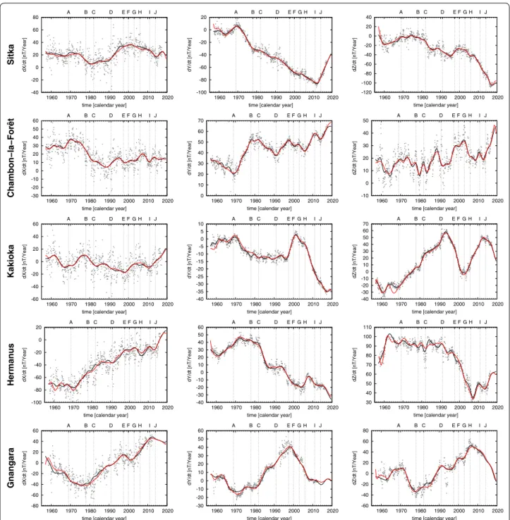
Figure 3 compares the observed and modeled secular
variation at different observatory sites. The model curves are derived from our preferred classical and kinematic field models. The observed secular variation series from ground-based geomagnetic observatories stop in 2017.5, as more recent data were not available at the time of this study.
The overall impression is that the classical and kin-ematic field models fit the observed secular variation
equally well. An exception is, at the model endpoints where the two curves deviate. Most likely, this is due to the endpoint constraint of the kinematic field models. The known jerk occurrences (A–J) are all clearly visible in the Y-component of Chambon-la-Forêt, whereas in other observatory data only some jerks are detectable, e.g., the series of Sitka shows only events in 1969 and 2011. Data of the Sitka observatory show large changes of the secular variation of Y and Z components in the past decade, that may be related to the rapid movement of the magnetic North Pole.
The same large similarity between the models can be
observed in Fig. 4, which shows six secular variation
coefficients with the largest amplitude of the two dif-ferent models. These coefficients largely determine the morphology of the secular variation at Earth’s surface.
Particularly, the coefficient h1
2 is closely related to the
prominent patch of reverse magnetic flux in the southern
hemisphere (Terra-Nova et al. 2017). Overall, differences
between the model coefficients rarely exceed 2 nT/year, except close to model endpoints, where models disperse largely.
Figure 4 also shows markers of known geomagnetic
jerks, to allow their identification in the evolution of the
secular variation coefficients. The coefficients ˙g0
1 and ˙h12
represent equatorial anti-symmetric contributions of the secular variation. These coefficients carry most of the known geomagnetic jerks, apart from the event in 1969
which is either not clearly visible in ˙g0
1 , or appears later in
1970. The identification of geomagnetic jerks in the equa-torial symmetric parts of the secular variation described
by ˙g1
1, ˙h11,˙g20 is less clear.
The temporally averaged secular variation spectra of
the two models are shown in Fig. 5. On large and small
scales, differences between spectra remain small at Earth’s surface. The spectra also indicate a very high tem-poral variability of the kinematic field secular variation at degrees 9 and 10, suggesting that at some epochs the
Table 1 Model diagnostics: residuals standard deviation in [nT/year] and damping parameters
Standard deviation [nT/year] Damping
X Y Z S T
Model 1 13.69 11.07 14.47 3.0d-10 3.0d-2
Model 2 12.42 10.89 13.89 see Model x3d
Table 3 0 20 40 60 80 100 120 140 160 180 200 1950 1960 1970 1980 1990 2000 2010 2020 √ dP rms differences [nT]
time [calendar year]
0 5 10 15 20 25 30 1950 1960 1970 1980 1990 2000 2010 2020 √dP rms differences [nT/yr]
time [calendar year] Fig. 2 Temporal evolution of the rms difference ( √dP ) of the main field (left) and secular variation (right) between models 1 and 2
power of the secular variation of these models is weaker by a few orders of magnitude than the secular variation of the classical field model.
At the core surface (Fig. 5, right) the spectral power
of the secular variation grows with spherical harmonic degree. The spectra of the two models start to deviate
from degree 11, where the spectrum of Model 2 flat-tens, whereas the spectrum of Model 1 continues to increase. We note the same high temporal variability at spherical harmonic degree 9 of the kinematic secular variation model. -40 -20 0 20 40 60 80 1960 1970 1980 1990 2000 2010 2020 A B C D E F G H I J dX/dt [nT/Year ]
time [calendar year]
Sitka -30 -20 -10 0 10 20 30 40 50 60 1960 1970 1980 1990 2000 2010 2020 A B C D E F G H I J dX/dt [nT/Year ]
time [calendar year]
Chambon−la−Forêt -60 -40 -20 0 20 40 60 1960 1970 1980 1990 2000 2010 2020 A B C D E F G H I J dX/dt [nT/Year ]
time [calendar year]
Kakioka -100 -80 -60 -40 -20 0 20 1960 1970 1980 1990 2000 2010 2020 A B C D E F G H I J dX/dt [nT/Year ]
time [calendar year]
Hermanu s -80 -60 -40 -20 0 20 40 60 1960 1970 1980 1990 2000 2010 2020 A B C D E F G H I J dX/dt [nT/Year ]
time [calendar year]
Gnangara -100 -80 -60 -40 -20 0 20 1960 1970 1980 1990 2000 2010 2020 A B C D E F G H I J dY/dt [nT/Year ]
time [calendar year]
0 10 20 30 40 50 60 70 1960 1970 1980 1990 2000 2010 2020 A B C D E F G H I J dY/dt [nT/Year ]
time [calendar year]
-40 -35 -30 -25 -20 -15 -10 -5 0 5 10 1960 1970 1980 1990 2000 2010 2020 A B C D E F G H I J dY/dt [nT/Year ]
time [calendar year]
-40 -30 -20 -10 0 10 20 30 40 50 60 1960 1970 1980 1990 2000 2010 2020 A B C D E F G H I J dY/dt [nT/Year ]
time [calendar year]
-30 -20 -10 0 10 20 30 40 50 60 1960 1970 1980 1990 2000 2010 2020 A B C D E F G H I J dY/dt [nT/Year ]
time [calendar year]
-120 -100 -80 -60 -40 -20 0 20 40 1960 1970 1980 1990 2000 2010 2020 A B C D E F G H I J dZ/dt [nT/Year]
time [calendar year]
-10 0 10 20 30 40 50 1960 1970 1980 1990 2000 2010 2020 A B C D E F G H I J dZ/dt [nT/Year]
time [calendar year]
-40 -30 -20 -10 0 10 20 30 40 50 60 70 1960 1970 1980 1990 2000 2010 2020 A B C D E F G H I J dZ/dt [nT/Year]
time [calendar year]
30 40 50 60 70 80 90 100 110 1960 1970 1980 1990 2000 2010 2020 A B C D E F G H I J dZ/dt [nT/Year]
time [calendar year]
-60 -40 -20 0 20 40 60 80 1960 1970 1980 1990 2000 2010 2020 A B C D E F G H I J dZ/dt [nT/Year]
time [calendar year]
Fig. 3 Observed and modeled secular variation at some observatory sites. From top to bottom: Sitka (Alaska), Chambon-la-Forêt (France), Kakioka (Japan), Hermanus (South Africa), Gnangara (Australia). The gray dots represent the observed monthly secular variation in X, Y and Z (from left to right). Solid curves display the modeled secular variation of Model 1 (black) and Model 2 (red). Vertical lines mark occurrences of geomagnetic jerks
4 6 8 10 12 14 16 18 20 22 24 26 1960 1970 1980 1990 2000 2010 2020 A B C D E F G H I J secular variation g 0 1 (nT/yr)
time [calendar year]
-35 -30 -25 -20 -15 -10 -5 0 5 1960 1970 1980 1990 2000 2010 2020 A B C D E F G H I J secular variation h 1 1 (nT/yr)
time [calendar year]
-35 -30 -25 -20 -15 -10 -5 0 1960 1970 1980 1990 2000 2010 2020 A B C D E F G H I J secular variation h 1 2 (nT/yr)
time [calendar year]
4 6 8 10 12 14 16 18 20 1960 1970 1980 1990 2000 2010 2020 A B C D E F G H I J secular variation g 1 1 (nT/yr)
time [calendar year]
-26 -24 -22 -20 -18 -16 -14 -12 -10 -8 1960 1970 1980 1990 2000 2010 2020 A B C D E F G H I J secular variation g 0 2 (nT/yr)
time [calendar year]
-28 -26 -24 -22 -20 -18 -16 -14 -12 -10 -8 1960 1970 1980 1990 2000 2010 2020 A B C D E F G H I J secular variation h 2 2 (nT/yr)
time [calendar year]
Fig. 4 Comparison of six modeled secular variation coefficients with the largest amplitude. Same colors are applied as in Fig. 3
10-3 10-2 10-1 100 101 102 103 104 5 10 15 Power [nT/yr 2 ]
spherical harmonic degree
104 105 106 107 108 5 10 15 Power [nT/yr 2 ]
spherical harmonic degree
Fig. 5 The temporally averaged secular variation spectra of Models 1 and 2 at Earth’s surface (left) and at the core surface (right). Same line styles are applied as in Fig. 3. The vertical bars indicate the range, i.e., the temporal variability of the individual spectra
Maps of the radial component of the magnetic field and its secular variation derived from Model 1 at the top
of the core are shown in Fig. 6. The radial magnetic field
component shows a dipole-dominated morphology, but with considerably small-scale features, such as reversed flux patches in both hemispheres. The secular varia-tion at the core surface tends to be dominated by small scales. Particularly notable features are low latitude pairs of opposite polarity secular variation which are typical
to advection (Amit 2014). Also note larger patches of the
radial secular variation in the vicinity of the magnetic North Pole, e.g., under Eastern Siberia.
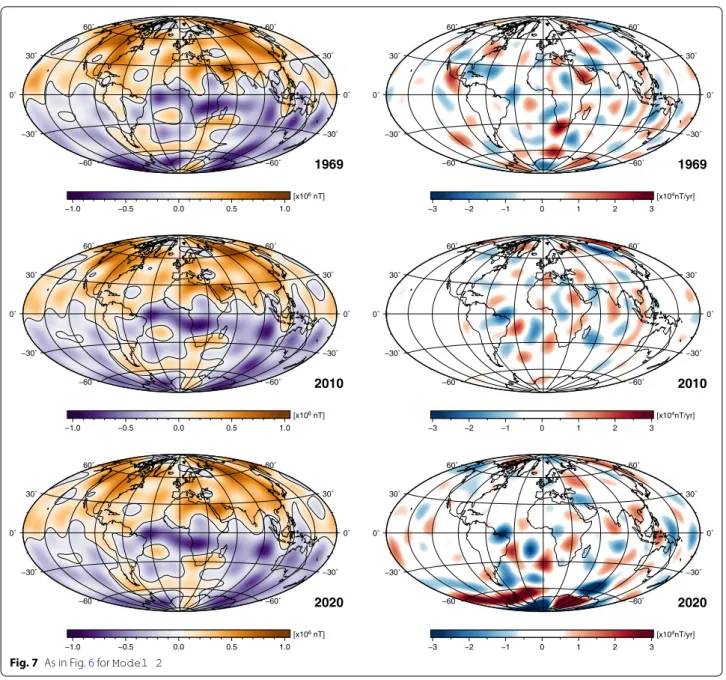
Figure 7 shows maps based on Model 2. Maps of the
radial component of the magnetic field at the core sur-face are widely in agreement with the respective maps
of Fig. 6. Perhaps most apparent, is the presence of the
reversed flux patch underneath the East Pacific, in both
models except at 1969 in Fig. 6. Maps of the secular
vari-ation in 2020 differ substantially, which may be due to the endpoint constraint of Model 2. The secular varia-tion map of Model 2 in 2020 contains some large-scale anomalously intense structures below the geographic South Pole, indicating an intensification of the flux in this region. Based on the strong secular variation at high
−60˚ −60˚ −30˚ −30˚ 0˚ 0˚ 30˚ 30˚ 60˚ 60˚ 1969 −1.0 −0.5 0.0 0.5 1.0 [x106 nT] −60˚ −60˚ −30˚ −30˚ 0˚ 0˚ 30˚ 30˚ 60˚ 60˚ 2010 −1.0 −0.5 0.0 0.5 1.0 [x106 nT] −60˚ −60˚ −30˚ −30˚ 0˚ 0˚ 30˚ 30˚ 60˚ 60˚ 2020 −1.0 −0.5 0.0 0.5 1.0 [x106 nT] −60˚ −60˚ −30˚ −30˚ 0˚ 0˚ 30˚ 30˚ 60˚ 60˚ 1969 −3 −2 −1 0 1 2 3 [x104nT/yr] −60˚ −60˚ −30˚ −30˚ 0˚ 0˚ 30˚ 30˚ 60˚ 60˚ 2010 −3 −2 −1 0 1 2 3 [x104nT/yr] −60˚ −60˚ −30˚ −30˚ 0˚ 0˚ 30˚ 30˚ 60˚ 60˚ 2020 −3 −2 −1 0 1 2 3 [x104nT/yr] Fig. 6 Radial component of the magnetic field at the core surface (left) and its secular variation (right) derived from Model 1 for epochs 1969, 2010 and 2020
latitudes of the northern hemisphere, Livermore et al.
(2017) inferred a zonal jet there. In the context of
equato-rial symmetry, they argued that such a zonal jet at high latitudes of the southern hemisphere would not produce detectable secular variation, because the field is oriented
in the east–west direction there. Indeed in Fig. 6 in 2020
the secular variation is very weak around the South Pole (and quite strong under the North Pole). All this makes the anomalously strong secular variation around the
South Pole in 2020 as seen in Fig. 7 quite suspicious.
However, secular variation maps of other epochs (1969
and 2010) are very similar to maps of Fig. 6, with
domi-nant small-scale features at mid- and low latitudes.
We conclude that classical and kinematic field models largely agree, both in spatial morphology as well as in the temporal evolution, but significantly deviate in their sec-ular variation towards the endpoints. The cause for this deviation is the constraint of the kinematic field model onto the flow acceleration, while the classical model gets along without such constraint.
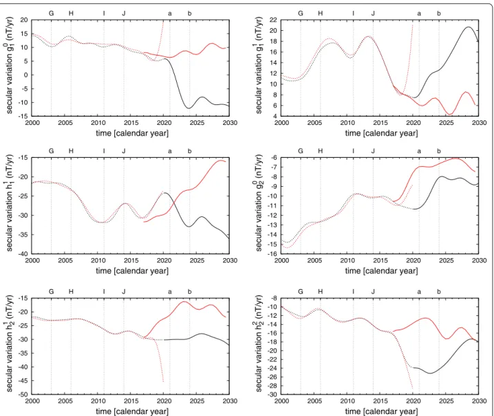
Direct secular variation forecast
Figure 8 displays observations and predictions of secular
variation coefficients with the largest amplitude at the
Earth surface, i.e., ˙g0
1,˙g11, ˙h11,˙g20, ˙h21, ˙h22 , from 2000 to 2030.
The most prominent feature of the forecast of Model 1
−60˚ −60˚ −30˚ −30˚ 0˚ 0˚ 30˚ 30˚ 60˚ 60˚ 1969 −1.0 −0.5 0.0 0.5 1.0 [x106 nT] −60˚ −60˚ −30˚ −30˚ 0˚ 0˚ 30˚ 30˚ 60˚ 60˚ 2010 −1.0 −0.5 0.0 0.5 1.0 [x106 nT] −60˚ −60˚ −30˚ −30˚ 0˚ 0˚ 30˚ 30˚ 60˚ 60˚ 2020 −1.0 −0.5 0.0 0.5 1.0 [x106 nT] −60˚ −60˚ −30˚ −30˚ 0˚ 0˚ 30˚ 30˚ 60˚ 60˚ 1969 −3 −2 −1 0 1 2 3 [x104nT/yr] −60˚ −60˚ −30˚ −30˚ 0˚ 0˚ 30˚ 30˚ 60˚ 60˚ 2010 −3 −2 −1 0 1 2 3 [x104nT/yr] −60˚ −60˚ −30˚ −30˚ 0˚ 0˚ 30˚ 30˚ 60˚ 60˚ 2020 −3 −2 −1 0 1 2 3 [x104nT/yr] Fig. 7 As in Fig. 6 for Model 2
is the steep decrease of ˙g0
1 by almost 15nT/year during a
very short interval of about 3 years. While this decrease is determined by the statistical properties of the time-series model, it may be difficult to accept this when con-sidering the past secular variation. In fact, this decrease would be caused by a large secular acceleration.
Advec-tive sources and sinks of ˙g0
1 exhibit a lot of cancellations
and it is the rather small residual that gives the historical
dipole decay (Olson and Amit 2006; Finlay et al. 2016),
i.e., subtle change in the core flow pattern and its
interac-tion with the field may yield considerable changes in g0
1 .
However, apparently such a change did not happen since 1840. The other terms vary within ranges of previous
oscillations (see Fig. 4).
Most of the secular variation terms of Model 1 indi-cate possible occurrences of two future geomagnetic
jerks in late 2020–early 2021, and in early 2024. In Fig. 8,
at these dates the predicted secular variation shows nota-ble changes in slope.
Kinematic secular variation forecast
The kinematic secular variation forecast is based on fore-casts of individual flow coefficients derived from a
multi-variate singular spectrum analysis (MSSA). Figure 9
shows the past and future temporal evolution of two
toroidal flow coefficients, t0
1, t30 . These coefficients are of
a particular interest, as they relate to changes in Earth’s
rotation (Jault et al. 1988; Jackson et al. 1993), which
-15 -10 -5 0 5 10 15 20 2000 2005 2010 2015 2020 2025 2030 G H I J a b secular variation g 0 1 (nT/yr)
time [calendar year]
-40 -35 -30 -25 -20 -15 2000 2005 2010 2015 2020 2025 2030 G H I J a b secular variation h 1 1 (nT/yr)
time [calendar year]
-50 -45 -40 -35 -30 -25 -20 -15 2000 2005 2010 2015 2020 2025 2030 G H I J a b secular variation h 1 2 (nT/yr)
time [calendar year]
4 6 8 10 12 14 16 18 20 22 2000 2005 2010 2015 2020 2025 2030 G H I J a b secular variation g 1 1 (nT/yr)
time [calendar year]
-16 -15 -14 -13 -12 -11 -10 -9 -8 -7 -6 2000 2005 2010 2015 2020 2025 2030 G H I J a b secular variation g 0 2 (nT/yr)
time [calendar year]
-30 -28 -26 -24 -22 -20 -18 -16 -14 -12 -10 -8 2000 2005 2010 2015 2020 2025 2030 G H I J a b secular variation h 2 2 (nT/yr)
time [calendar year]
Fig. 8 Comparison of six observed and predicted secular variation coefficients with the largest amplitude at Earth’s surface. Model 1 (dashed black line), Model 2 (dashed red line) and their forecasts (solid lines). Vertical lines labeled with a and b mark two possible geomagnetic jerks. The other labels mark occurrences of known jerks
coincide with geomagnetic jerks (Holme and de Viron
2005; Wardinski et al. 2008).
The MSSA of the temporal flow variability is trun-cated at the degree where past model and forecast of the flow coefficients becomes almost continuous, which is achieved for a truncation level k = 22 , i.e., the first 22 eigenmodes. Both flow coefficients show spurious accel-erations from 2017 on, which is caused the endpoint
constraint of the flow acceleration, cf. (23). Therefore, we
consider the kinematic field and flow coefficients to be flawed and start the kinematic forecast from 2017.
Figure 8 also provides a comparison between the direct
and kinematic forecasts of secular variation coefficients. The kinematic forecast starts in 2017 to reduce the influ-ence of the model’s faulty temporal behavior close to its endpoint. These forecasts differ by their temporal evolu-tion to those of the direct secular variaevolu-tion forecast. Most
apparent are these differences in the forecast of ˙g0
1 , where
both forecasts have opposite signs and differ by about 20 nT/year. The kinematic forecast predicts a gently varying
˙
g10 . This forecast discrepancy is also clearly seen for ˙g10, ˙g11
and ˙h1
2 . However, these forecasts show also common
fea-tures related to future geomagnetic jerks. The cause for the forecast discrepancy is not understood, and it is not in relation to the anomalous flow acceleration at the kin-ematic model endpoint, as the kinkin-ematic forecast starts a few years prior to the model’s endpoint.
Predictability
Previous studies (Aubert 2015; Whaler and Beggan 2015)
used rms-based measures (31) to quantify differences
between a reference model and forecasts. The reference model is a model for the epoch 2017 of the classical and kinematic model branches and labeled as M1 2017 and M2 2017, respectively.
Table 2 lists the rms-differences between different
epoch models of Model 1 and Model 2. Generally,
the rms-differences of the direct secular variation fore-casts (Model 1) is smaller than those of the kinematic forecasts. However, it is not clear whether it allows to conclude upon the performance of the forecasts. Glob-ally, it suggests that the main field and secular variation of Model 1 tend to be more similar over longer time intervals than for Model 2. This may agree with results
based on numerical dynamos (Hulot et al. 2010) and data
assimilation using numerical dynamos (Aubert 2015).
Their studies used rms-based error estimates, and their results suggested a possible predictability of several dec-ades to a century.
We perform several prediction experiments to meas-ure the prediction length of the first 26 secular variation coefficients for different prediction setups. In these set-ups, the starting of the forecast is set to 1995, 2005 and 2015, respectively. The forecast period is in all cases 10
years, for which we compute the sAPE(t) , cf. (30).
First, it is found for the direct secular variation forecasts of the classical field model that the prediction length is largely independent of the number of eigenvalues consid-ered in the MSSA forecast. Merely, this number has to be larger than the number of significant eigenvalues.
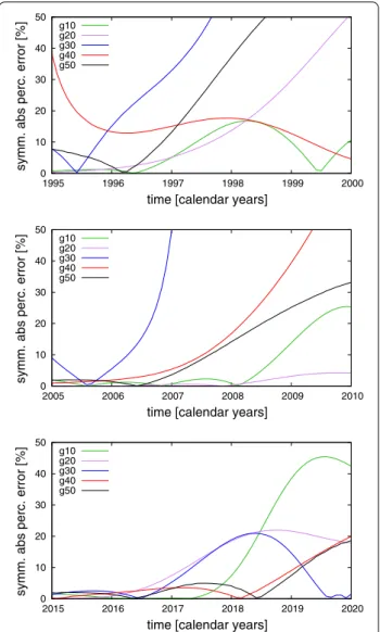
Results of the forecast experiments are shown
in Figs. 10 and 11. Generally, the prediction error
(sAPE(t)) of the zonal secular variation coefficients
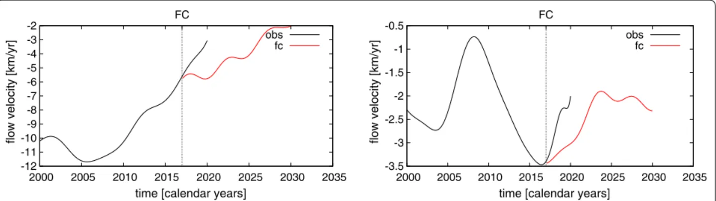
-12 -11 -10 -9 -8 -7 -6 -5 -4 -3 -2 2000 2005 2010 2015 2020 2025 2030 2035 FC
flow velocity [km/yr]
time [calendar years]
obs fc -3.5 -3 -2.5 -2 -1.5 -1 -0.5 2000 2005 2010 2015 2020 2025 2030 2035 FC
flow velocity [km/yr]
time [calendar years]
obs fc
Fig. 9 Evolution of the toroidal flow coefficients t0
1 (left) and t 0
3 (right); their past variations (black) and their forecasts (red) based on the MSSA. The
vertical line labeled with FC marks the start of the forecast
Table 2 The rms differences between models of different epochs and Model 1 and Model 2
Differences of main field models are given in [nT] and differences of secular variation models are in [nT/year]
Main field Secular variation
M1 2017 M2 2017 M1 2017 M2 2017
2020 271.41 863.49 21.00 22.11
2025 306.11 1511.43 34.70 40.79
increases with time, except for the prediction of ˙g0 4 of
the 1995-experiment which improves with time. It is also noted that prediction error of the 2015-experi-ment is mostly smaller than for the other experi2015-experi-ments
(Fig. 10). We focus on the prediction of the large-scale
secular variation represented by the first coefficients. For practical purposes, we arbitrarily examine the first 26 coefficients. The mean prediction length for which the prediction error sAPE(t) < 10% of the first 26
secu-lar variation coefficients is around 3 years (Fig. 11). This
is substantially shorter than results by Aubert (2015),
who found a possible predictability of a century. Similar experiments are performed for the flow fore-casts of the kinematic field model (Model 2), with the
resulting prediction lengths shown in Fig. 12. The mean
prediction length for all experiments is always shorter than 2.5 years, i.e., shorter than the mean prediction
length of direct secular variation forecasts (Fig. 11).
However, we note that the prediction length of t0
1 for
experiments started in 1995 and 2005 is longer or equal to 5 years, and that only the forecast deteriorates only when the experiment is started closer to the model endpoint.
We avoided performing such experiments for the kin-ematic secular variation forecast, because of the faulty 0 10 20 30 40 50 1995 1996 1997 1998 1999 2000
symm. abs perc. error [%]
time [calendar years]
g10 g20 g30 g40 g50 0 10 20 30 40 50 2005 2006 2007 2008 2009 2010
symm. abs perc. error [%]
time [calendar years]
g10 g20 g30 g40 g50 0 10 20 30 40 50 2015 2016 2017 2018 2019 2020
symm. abs perc. error [%]
time [calendar years]
g10 g20 g30 g40 g50
Fig. 10 Evolution of the sAPE(t) of zonal secular variation coefficients based on Model 1 of the three forecasts experiments started in 1995 (top panel), in 2005 (middle panel) and in 2015 (bottom panel), respectively 0 1 2 3 4 5 6 7 0 5 10 15 20 25 1 2 3 4 5
prediction length [years]
coefficient number mean PL 0 1 2 3 4 5 6 7 0 5 10 15 20 25 1 2 3 4 5
prediction length [years]
coefficient number mean PL 0 1 2 3 4 5 6 0 5 10 15 20 25 1 2 3 4 5
prediction length [years]
coefficient number
mean PL
Fig. 11 Prediction lengths defined by the time interval when sAPE(t) < 10% of different forecast experiments base on Model 1 with
forecasts started in 1995 (top panel), in 2005 (middle panel) and in 2015 (bottom panel), respectively. The solid horizontal red lines represent mean prediction lengths in years derived from the first 26 secular variation coefficients, i.e., ˙g0
1. . . ˙g 1
5 . Top axes indicate degrees
temporal behavior of Model 2 close to its endpoints. This behavior is caused by the constraint that controls
the flow acceleration at the model endpoints by E .
Constraining the flow acceleration too strongly leads to a very small flow acceleration, which is as unrealis-tic as the counter case with large flow acceleration. To this end, conclusions about the flow acceleration at the endpoints are loose, and in the future we may constrain secular variation of kinematic field models to be similar to the secular variation of the classical model.
Derivation of candidate models
Our candidate models for the DGRF 2015, IGRF 2020, and the secular variation for the period 2020 to 2025 are derived from Model 1 and its respective forecast. This is justified by the large resemblance of the main field description of two models. The candidates for the DGRF 2015 and IGRF 2020 are given by the main field model in 2015.0 and 2020.0, respectively, truncated at spherical harmonic degree 13, in nT with two decimal places. The candidate of the secular variation model is given by the forecast for the epoch 2022.5 truncated to spherical har-monic degree 8.
Conclusion
We derive field models for the period 1957 to 2020 from ground-based geomagnetic observatory data as well as satellite-based virtual observatory data. These models are constructed using two different techniques, a clas-sical modeling (Model 1) that provides an optimal fit to observations, and a data assimilation to a dynamical assumption of Earth’s core flow (Model 2). These strate-gies provide similar results for the core field and its tem-poral variations over the past decades.
In this study we set up two forecasting schemes that rely on analyses of multi-variate time series of secular variation coefficients. We derived time-series models of the field variability, from which forecasts of individual secular variation coefficients are obtained. These serve as direct secular variation predictions. Prediction experi-ments indicate a robust forecast of the secular variation of about three years. This might be a lower boundary and is determined by our cautious definition of the prediction length; the time interval when sAPE(t) < 10%.
Forecasts of the flow coefficients are derived in the same manner and used in forward calculations of the secular variation due to advection in the core, where con-tributions from magnetic diffusion are neglected and a tangential geostrophy assumption couples the toroidal and poloidal flows (kinematic secular variation forecast). This approach extends beyond the approach of Beggan
and Whaler (2010); Whaler and Beggan (2015) which
used steady and constantly accelerated flow to predict future secular variation. However, our kinematic secu-lar variation forecast suffers from faulty estimates of the core flow at the model endpoints due to a possibly inac-curate restriction of the flow acceleration. Therefore, the latter approach may not provide robust forecasts of the secular variation, unless the endpoint constraint can be dropped. Interestingly, both strategies consistently indi-cate the occurrence of future geomagnetic jerks in 2021 and 2024. The uncertainty in the exact timing of these events is related to the original temporal resolution of our data, which is optimistically smaller than ±1 year 0 1 2 3 4 5 6 7 8 9 10 0 5 10 15 20 25 1 2 3 4 5
prediction length [years]
coefficient number mean PL 0 1 2 3 4 5 0 5 10 15 20 25 1 2 3 4 5
prediction length [years]
coefficient number mean PL 0 1 2 3 4 0 5 10 15 20 25 1 2 3 4 5
prediction length [years]
coefficient number
mean PL
Fig. 12 Prediction lengths for the first 26 toroidal flow coefficients estimated from different forecast experiments with forecasts started in 1995 (top panel), in 2005 (middle panel) and in 2015 (bottom panel), respectively. The solid horizontal red lines represent mean prediction lengths in years derived from the first 26 toroidal flow coefficients. Top axes indicate degrees of the spherical harmonic expansion
and realistically larger than ±6 months, as well as to the strength of the temporal constraint.
Of course, our strategies of forecasting are limited by the lack of observations from within the (geodynamo) system (which are not available), but not by inferences made upon the geodynamo. Similar limitations may occur to approaches using a full description of the dynamo in a data assimilation framework to forecast
geo-magnetic secular variation, like Aubert (2015), Fournier
et al. (2015). We hypothesize that when longer time series
are considered, a longer behavior of the field can be mod-eled; however, this will not improve the predictability of the short-term (decadal) field variations, as they may be chaotic.
To this end, results of the classical modeling (Model 1) are used to provide candidates for the definitive geo-magnetic reference field model (DGRF) in 2015, and IGRF candidate model for 2020. The candidate of the sec-ular variation model is given by the forecast for the epoch 2022.5.
Abbreviations
CMB: Core–mantle boundary; DGRF: Definitive geomagnetic reference field; IAGA : International Association of Geomagnetism and Aeronomy; IGRF: Inter-national Geomagnetic Reference Field; MSSA: Multi-variate singular spectrum analysis; sAPE: Symmetric absolute prediction error; VO: Virtual geomagnetic observatory.
Acknowledgements
The authors would like to record their gratitude to scientists working at magnetic observatories, data suppliers and involved national institutes for making geomagnetic observatory data available, to the World Data Centre for Geomagnetism (Edinburgh) for compiling these data in a database and to the International Service of Geomagnetic Indices for making data products (indices) available. The authors acknowledge ESA for providing access to Swarm Level 1b products. We also would like to thank V. Lesur for sharing his satellite-based geomagnetic field model before its submission. This work was supported by CNES. The critical reading and very valuable comments by two anonymous reviewers are appreciated.
Authors’ contributions
IW organized the manuscript based on the analyses of the contributing co-authors. All authors contributed modeling results and/or detailed technical analyses and/or discussions for this study. All authors read and approved the final manuscript.
Funding
IW was funded at an initial state of this study by the ESA project 3D-Earth and by the Centre National des Etudes Spatiales (CNES) within the context of the project “Exploitation des mesures de la mission Swarm”. DS was funded by CNES project “Exploitation des mesures de la mission Swarm”. HA acknowl-edges financial support from “Programme National de Planétologie” of “Institut national des sciences de l’Univers”. AC acknowledges financial support from CNES over the project “Indices d’Activité Magnétique : Météorologie de l’Espace et Géomagnétisme Spatial”. This work was supported by CNES. Data availability statement
The datasets used and/or analyzed during the current study are available from the corresponding author on reasonable request.
Competing interests
The authors declare that they have no competing interests.
Author details
1 Institut de Physique du Globe de Strasbourg, Université de Strasbourg/EOST,
CNRS, UMR 7516, Strasbourg, France. 2 Laboratoire de Planétologie et
Géody-namique, Université de Nantes, Université d’Angers, CNRS, UMR 6112, Nantes, France. 3 Centre National d’ Etudes Spatiales (CNES), Paris, France. 4 Laboratoire
Magmas et Volcans, Université de Clermont Auvergne, CNRS UMR 6524, Clermont Ferrand, France.
Appendix A: Theory of singular spectrum analysis
We briefly recall some aspects of the singular spectrum analysis (SSA). The SSA is a non-parametric spectral esti-mation method that incorporates aspects of classical time-series analysis, signal processing, multi-variate statistics
and geometry (Vautard et al. 1992; Golyandina et al. 2001).
We first formulate the theoretical concepts for uni-variate time series, and then extend them to multi-variate time series. For a deeper review and also its application to a variety of phenomena in meteorology, oceanography and
climatology we refer to Ghil et al. (2002) and references
therein.
Uni‑variate analysis
The analysis is based on the embedding of a time series yt
in a vector space of dimension M that determines the long-est periodicity captured by the analysis. The spectral infor-mation on a time series are obtained by diagonalizing the
M× M covariance matrix Cy of yt . The covariance matrix
Cy can be estimated directly from the data, i.e., its entries cij
depend only on the lag δ = |i − j|:
Usually, the decomposition of the covariance matrix Cy
in q orthogonal eigenvectors Eq that are called temporal
empirical orthogonal functions (EOF) is done by
singu-lar value decomposition. The eigenvalues ǫq of Cy account
for the partial variance in the direction Eq and the sum of
the eigenvalues, i.e., the trace of Cy , gives the total
vari-ance of the original time series yt . By a projection of the
time series onto the EOF the temporal principal
compo-nent Ak
t can be obtained:
In fact, this method decomposes the time series in parts that correspond to trends, oscillatory modes or noise. Therefore, it allows the time series to be reconstructed and to be forecasted by using linear combinations of the temporal principal components and EOFs. The
recon-structed components Rk t are given by (A.1) cij= 1 N− δ N−δ t=1 yt· yt+δ. (A.2) Akt = M j=1 X(t+ j − 1)Ek(j).
where K is the set of k EOFs and temporal principal com-ponents on which the reconstruction is based. We refer to k as the truncation level of the reconstruction and forecast. This truncation level is k ≤ q . The values of the
normalization factor Nt , as well as of the lower and upper
bound of summation Lt and Ut , differ between the central
part of the time series and in the vicinity of its endpoints
(Ghil et al. 2002).
An oscillatory mode is characterized by a pair of nearly equal eigenvalues and by associated principal components
that are in approximate phase quadrature (Ghil et al. 2002).
Such a pair can represent a non-linear, non-harmonic oscil-lation, because a single pair of eigenmodes are more sen-sitive to the basic periodicity of an oscillatory mode than methods with fixed basis functions, such as the sines and cosines used in the Fourier transform.
Multi‑variate analysis
The multi-variate (or multi-channel) singular spectrum analysis (MSSA) is a generalization of the SSA from uni-variate to multi-uni-variate time series, such as time series of individual Gauss coefficients. Its use was proposed theo-retically in the context of non-linear dynamics
(Broom-head and King 1986) and numerous examples of successful
application of this methods can be found, e.g., Plaut and
Vautard 1994.
The MSSA allows the identification of dynamically rele-vant temporal patterns that are coherent in series that form a multi-variate time series. These individual series are often called channels. By analogy to the SSA, each of L-channel
data vectors yl,t : l = 1, . . . , L, t = 1, . . . , N is expanded
to a state vector
for each channel l = 1, . . . , L , and the window length M.
Following the approach of Broomhead and King (1986);
Allen and Robertson (1996), then the MSSA relies on the
construction a grand covariance matrix Cx like
(A.3) Rkt = 1 Nt k∈K Ut j=Lt Ak(t− j + 1)Ek(j), (A.4) Yl = yl,1 yl,2 . . . yl,M yl,2 yl,3 . . . yl,M+1 . . . ... yl,N−M . . . yl,N−1 yl,N−M+1 . . . yl,N (A.5) Cx= 1 N− M + 1Y TY = C11 C12 C13 . . . C1L C22 C23 . . . C2L C33 . . . C3L . .. ... CLL ,
where each block Cll′ is a covariance matrix between
channels l and l′ . The blocks C
ll′ have the entries
The LM × LM matrix Cx is symmetric and by
diagonaliz-ing, LM eigenvectors Ek : k = 1, . . . , LM can be obtained.
The eigenvectors are composed of L consecutive
seg-ments with length M. Similarly to (A.2) the associated
principal components Ak can be computed by
project-ing Y in the directions of the eigenvectors (i.e. onto the EOFs):
El,k(j) are the elements of the eigenvectors. The Ak(t) are
single-channel time series and likewise to (A.3) the kth
reconstruction of the signal of channel l can be obtained by:
where LT and Ut are the lower and upper bound of
sum-mation, respectively.
Figure 13 shows the first 12 eigenvectors of the toroidal
flow decomposition. Clearly, the first two eigenvectors capture the slow variation of flow coefficients, whereas other eigenvectors represent the shorter temporal varia-tions of the flow. The first few eigenvectors explain nearly the entire signal variance, which is given on top of each single plot. However, higher indexed eigenvectors also show non-zero partial variance, suggesting that these eigenvectors may carry relevant temporal information.
An important aspect of the analysis is how well com-ponents of the time series are separated from each other. The components generally group in two disjunctive parts, one corresponds to the signal, the other to the noise. The signal could be composed of slowly varying, periodic and/or quasi periodic components. A way to measure the separation between components, is to calculate the weighted correlation or w-correlations, as given by
Goly-andina et al. (2001).
In Fig. 14, the so-called, w-correlation matrix is
dis-played. It shows the weighted correlations for
princi-pal components, Ak , of the temporal flow variability.
Accordingly, large values of w-correlation exist for diagonal elements of the matrix, where individual modes correlate with themselves (dark red color). Whereas, small values of the w-correlation (lighter
(A.6) (Cll′)j,j′= 1 N− M + 1 N−M+1 t=1 Ytl+j−1Ytl+j′−1. (A.7) Akt = M j=1 L l=1 Ytl+j−1El,k(j). (A.8) Rl,kt = 1 Mt Ut j=Lt Ak(t− j + 1)El,k(j),