SOFTWARE RELIABILITY TREND ANALYSES: FROM THEORETICAL TO PRACTICAL CONSIDERATIONS

HAL Id: hal-01978842

https://hal.laas.fr/hal-01978842

Submitted on 11 Jan 2019

HAL is a multi-disciplinary open access

archive for the deposit and dissemination of sci-entific research documents, whether they are pub-lished or not. The documents may come from teaching and research institutions in France or abroad, or from public or private research centers.

L’archive ouverte pluridisciplinaire HAL, est destinée au dépôt et à la diffusion de documents scientifiques de niveau recherche, publiés ou non, émanant des établissements d’enseignement et de recherche français ou étrangers, des laboratoires publics ou privés.

SOFTWARE RELIABILITY TREND ANALYSES:

FROM THEORETICAL TO PRACTICAL

CONSIDERATIONS

Karama Kanoun, Jean-Claude Laprie

To cite this version:

Karama Kanoun, Jean-Claude Laprie. SOFTWARE RELIABILITY TREND ANALYSES: FROM THEORETICAL TO PRACTICAL CONSIDERATIONS. IEEE Transactions on Software Engineer-ing, Institute of Electrical and Electronics Engineers, 1994, 20, pp.740 - 747. �hal-01978842�

IEEE Transactions on Software Engineering, Vol 20, No 9, 1994, pp 740-747

S

R

T

A

:

F

T

T

P

C

Karama KANOUN and Jean-Claude LAPRIE

LAAS-CNRS, 7, avenue du Colonel Roche, 31077 Toulouse (France) e-mail: kanoun@laas.fr — laprie@laas.fr

Phone: +(33) 61 33 62 00 — Fax: +(33) 61 33 64 11

Abstract

This paper addresses the problem of reliability growth characterization and analysis. It is intended to show how reliability trend analyses can help the project manager in controlling the progress of the development activities and in appreciating the efficiency of the test programs. Reliability trend change may result from various reasons, some of them are desirable and expected (such as reliability growth due to fault removal) and some of them are undesirable (such as slowing down of the testing effectiveness). Identification in time of the latter allows the project manager to take the appropriate decisions very quickly in order to avoid problems which may manifest later.

The notions of reliability growth over a given interval and local reliability trend change are introduced through the subadditive property, allowing better definition and understanding of the reliability growth phenomena; the already existing trend tests are then revisited using these concepts. Emphasis is put on the way trend tests can be used to help the management of the testing and validation process and on practical results that can be derived from their use; it is shown that, for several circumstances, trend analyses give information of prime importance to the developer.

Index terms:

Reliability growth, trend tests, trend analysis, validation management.

* _{The work reported in this paper was partially supported by the ESPRIT Basic Research Action on Predictably}

Dependable Computing Systems (Action no. 6362).

1. Introduction

Generally, software reliability studies are based on reliability growth models application in order to evaluate the reliability measures. When performed for a large base of deployed software systems, the results are usually of high relevance (see e.g. [1, 10] for examples of such studies). However, utilization of reliability growth models during early stages of development and validation

is much less convincing: when the observed times to failure are of the order of magnitude of minutes or hours, the predictions performed from such data can hardly predict mean times to failure different from minutes or hours … which is so distant of any expected reasonable reliability. In addition, when a program under validation becomes reliable enough, the times to failure may simply be large enough in order to make impractical the application of reliability growth models to data belonging to the end of validation only, due to the (hoped for) scarcity of failure data. On the other hand, in order to become a true engineering exercise, software validation should be guided by quantified considerations relating to its reliability. Statistical trend tests for trend analysis provide such guides. It is worth noting that trend analyses are generally carried out by most of the companies during software testing [8, 19, 20]. However they are usually applied in an intuitive and empirical way rather than in a quantified and well defined method.

The work presented in this paper is an elaboration on the study carried out in [12], which focused on experimental data. In this paper, the discussion of these experimental data is more detailed, it is preceded by developments on the very notion of reliability growth. Emphasis is first put on the characterization of reliability growth via the subadditive property and its graphical interpretation. Then, the already existing reliability growth tests (mainly the Laplace test) are briefly presented and their relationship with the subadditive property outlined. The way trend tests can be used to help the management of the validation process is then addressed before illustration on three data sets issued from real-life systems.

The paper is composed of five sections. Section 2 is devoted to formal and practical definitions of reliability growth. In Section 3, some trend tests are presented and discussed; the type of results which can be drawn from trend analysis are stated. Section 4 is devoted to exemplifying the results from Sections 2 and 3 on failure data collected on real-life systems.

2. Reliability growth characterization

Software lack of reliability stems from the presence of faults, and is manifested by failures which are consecutive to fault sensitization1_{. Removing faults should result in reliability growth.}

However, it is not always so, due to the complexity of the relation between faults and failures, thus between faults and reliability, which has been noticed a long time ago (see e.g., [16]). Basically, complexity arises from a double uncertainty: the presence of faults and the fault sensitization via the trajectory in the input space of a program2_{. As a consequence, one usually observes reliability trend}

changes, which may result from a great variety of phenomena, such as i) the variation in the utilization environment (variation in the testing effort during debugging, change in test sets,

1 _{For a precise definition of faults, failures, reliability, etc. see [15].}

addition of new users during the operational life, etc.) or ii) the dependency between faults (some faults can be masked by others, they cannot be activated as long as the latter are not removed [18]).

Reliability decrease may not, and usually does not, mean that the software has more and more faults; it does just tell that the software exercises more and more failures per unit of time under the corresponding conditions of use. Corrections may reduce the failure input domain but more faults are activated or faults are activated more frequently. However, during fault correction, new faults may be also introduced — regression faults — which can deteriorate or not software reliability depending on the conditions of use. Last but not least, reliability decrease may be consecutive to specification changes, as exemplified by the experimental data reported in [14].

2.1. Definitions of reliability growth

A natural definition of reliability growth is that the successive inter-failure times tend to become larger, i.e., denoting T1, T2,… the sequence of random variables corresponding to inter-failure times:

T_i ≤

st Tj, for all i < j, (1)

where ≤_st means stochastically smaller than (i.e., P{Ti <v} ≥ P{Tj <v} for all v > 0). Under the stochastic independency assumption, relation (1) is equivalent to, letting FTi(x) denote the

cumulative distribution function of Ti:

FTi(x) ≥ FTj(x) for all i < j and x > 0 (2)

An alternative to the (restrictive) assumption of stochastic independency is to consider that the successive failures obey a non-homogeneous Poisson process (NHPP). Let N(t) be the cumulative number of failures observed during time interval [0, t], H(t) = E[N(t)] its mean value, and

h(t) = dH(t)/dt its intensity, i.e. the failure intensity. A natural definition of reliability growth is then that the increase in the expected number of failures tends to become lower, i.e. that H(t) is concave, or, equivalently, that h(t) is non-increasing. There are however several situations where even though the failure intensity fluctuates locally, reliability growth may take place on average on the considered time interval3_{. An alternative definition allowing for such local fluctuations is then that}

the expected number of failures in any initial interval (i.e. of the form [0, t]) is no lower than the expected number of failures in any interval of the same length occurring later (i.e. of the form [x, x+t]). The independent increment property of an NHPP enables to write this later definition as:

H(t1) + H(t2) ≥ H(t1+t2) for all t1,t2 ≥ 0 and 0 ≤ t1+t2 ≤ T (3)

inequality is presumed strict for at least one couple (t1,t2). When relation (3) holds, the function is

said to be subadditive over [0,T] (see e.g. [9]). When relation (3) is reversed for all t1,t2 ≥ 0 and

3 _{The NHPP assumption (more precisely the property of independent increments) is fundamental since a stationary}

process which is a non-Poisson process may undergo transient oscillations that are impossible to be distinguished from a trend in a non-stationary Poisson process (see for instance [2, p. 25] or [7, p. 99] for renewal processes).

0 ≤ t1+t2 ≤ T, the function is said to be superadditive indicating reliability decrease on average over

[0,T]. This relation is very interesting since it allows for local fluctuations: locally sub-intervals of reliability decrease may take place without affecting the nature of the trend on average (over the considered time interval). For instance, when h(t) is strictly decreasing over [0, T] relation (3) is verified but the converse is not true. This is detailed in the next sub-section.

2.2. Graphical interpretation of the subadditive property

In this section, we will derive a graphical interpretation of the subadditive property and show the link between this property and several situations of reliability growth and reliability decrease.

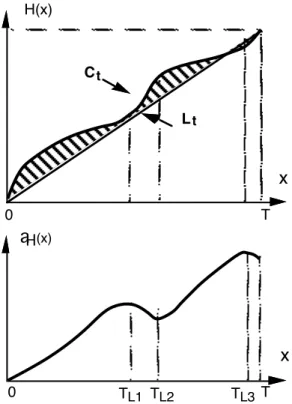
Let C_t denote the portion of the curve representing the cumulative number of failures in [0, t] as indicated in figure 1 and Lt the line joining the two ending points of Ct (i.e., the chord from the origin to point (t, H(t)) of C_t). Let A[Ct] denote the area delimited by Ct and the coordinate axis, A[Lt] denote the area delimited by Lt and the coordinate axis and aH(t) the difference between these two areas: aH(t) = (A[Ct] - A[Lt]). With these notations, relation (3) becomes:

aH(t) = (A[Ct] - A[Lt]) ≥ 0 for all t ∈ [0, T] (4)

Lt Ct T x H(x) 0 T x 0 TL1 TL2 TL3 a_H(x)

Figure 1: Graphical interpretation of the subadditive property

Let us divide the interval [0, t] in K small time intervals of length dt, i.e., t = K dt. K may be either even or odd. Let us consider the even case. In relation (3), let t1 take successively the values

{0, dt, 2dt, 3dt, … K/2 dt } and t2 = t - t1. Relation (3) becomes successively:

H(0) + H(Kdt) ≥ H(t) H(dt) + H((K-1)dt) ≥ H(t) …

H(K_{2 dt) + H(}K_{2 dt) ≥ H(t)}

Summing over the K_{2 +1 inequalities gives:}

∑

H(jdt) + H(K_{2 dt) ≥ (} K_{2 +1 )H(t)}

Replacing K by t/dt and taking the limit when dt approaches zero lead to: ⌡⌠ 0

t

H(x) dx ≥ _{2 H(t). The} t left term corresponds to the area of the region delimited by C_t and the coordinate axis and the right term to the area of the region between Lt and the coordinate axis. Relation (3) is thus equivalent to: ⌡

⌠ 0

t

H(x) dx - _{2 H(t) ≥ 0. That is: a}t _H(t) ≥ 0.

When K is odd derivation can be handled in a similar manner. ❑ End of proof

With this graphical representation, the identification of the subadditive property becomes very easy. For instance, the function considered in Fig. 1 is subadditive over [0, T]: there is reliability growth over the whole time interval even though local fluctuations take place in the meantime.

It is worth noting that, given a subadditive function, when t varies from 0 to T the difference between the two areas, aH(t), may increase, decrease or become null without being negative in any case. It is positive increasing at the beginning and:

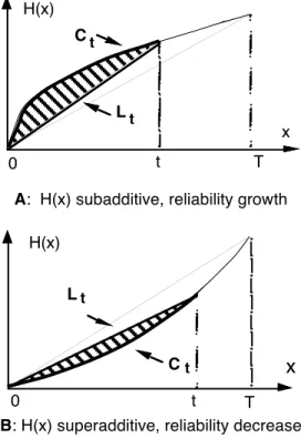
• without local reliability fluctuation, the cumulative number of failures curve is concave leading to a positive increasing aH(t) (see Fig. 2, case (a)),

• in case of local reliability fluctuation, the difference between the two areas takes its first maximum when the chord from the origin to point (t, H(t)) of Ct is tangent to Ct; let TL denote this point; from T_L, aH(t) is decreasing until the next point where the chord is tangent to Ct and so on.

Considering again the case of local reliability fluctuation of Fig. 1, the existence of point TL is due to the change in the concavity of the curve giving the cumulative number of failures, more precisely, it takes place after the point of concavity change. Taking TL as the time origin, would lead to a superadditive function from TL to the following point of local trend change (since the curve giving the cumulative number of failures is convex over this time interval). This is illustrated on Fig. 1 where the function considered has two sub-intervals of local reliability decrease (namely,

intervals [TL1, TL2] and [TL3, T]) in spite of reliability growth on the whole interval [0, T] since the function is subadditive over [0, T].

What precedes is true for a superadditive function also:

• without local reliability fluctuation, the cumulative number of failures curve is convex leading to a negative aH(t) (Figure 2, case B),

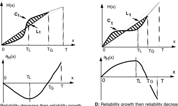
• in case of local reliability fluctuation, aH(t) takes its first minimum at TL where the chord is tangent to Ct; from TL, aH(t) is increasing until the next point of local trend change and so on. There are however more complicated situations where the cumulative number of failures is neither subadditive nor superadditive over the considered interval. For these cases, a change in the time origin is thus needed. Two such situations are illustrated in Figure 3.

For situation C, before TG the function is superadditive denoting reliability decrease over [0, TG]. TG corresponds to the point where the sign of aH(t) changes: the function is no more superadditive. TL corresponds to the region where aH(t) is no more decreasing denoting local trend change, however the function continues to be superadditive until point TG. On the sub-interval of time between TL and T the curve is concave indicating reliability growth over [TL, T]. Situation D is the converse of situation C: until point TG the cumulative number of failures is subadditive denoting reliability growth over [0, TG]; from TG, it is no more subadditive. On [TL, T] the function is superadditive corresponding to reliability decrease over this time interval. Combining situations C and D leads to interesting situations where the trend changes more than once.

0 t T

L_t C_t H(x)

x

A: H(x) subadditive, reliability growth

0 C_t L_t T t x H(x)

B: H(x) superadditive, reliability decrease

Lt C_t T x T_G TL H(x) 0 0 T x T_G TL aH(x)

C: Reliability decrease then reliability growth

0 H(x) C t L t T x TG TL aH(x) 0 _T x G TL T

D: Reliability growth then reliability decrease

Figure 3: Subadditivity / superadditivity and local trend variation

What precedes shows that the notion of reliability growth as defined by the subadditive property is related to the whole interval of time considered and is, as thus, strongly connected with the origin of the time interval.

Finally, it is worth while to point out an interesting situation which may be encountered for real systems: the case where the difference between the two areas, aH(t), is constant (or null) over a given interval, say [t1, t2]. This is characterized by the fact that the derivative of aH(t) given by relation (5) is null over [t1, t2].

d dt aH(t) = d dt

[

]

[

]

Integration of (5) leads to a linear cumulative number of failures function, i.e., a constant failure intensity over [t1, t2]. The constancy of aH(t) over a given time interval indicates thus stable reliability over this time interval.

3. Trend Analysis

Reliability growth can be analyzed through the use of trend tests. We will present only the most used and significant trend tests in this section and put emphasis on the relationship between the Laplace test (the most popular one) and the subadditive property. The presentation of the tests is followed by a discussion on how they can be used to follow up software reliability.

Failure data can be collected under two forms: inter-failure times or number of failures per unit

of time. These two forms are related: knowing the inter-failure times it is possible to obtain the

number of failures per unit of time (the second form needs less precise data collection). The choice between one form or the other may be guided by the following elements: i) the objective of the

reliability study (development follow up, maintenance planning or reliability evaluation), ii) the way data are collected (data collection in the form of inter-failure times may be tedious mainly during earlier phases of the development, in which case it is more suitable and less time consuming to collect data in the form of number of failures per unit of time) and iii) the life cycle phase concerned by the study. Using data in the form of "number of failures per unit of time" reduces the impact of very local fluctuations on reliability evaluation. The unit of time is a function of the type of system usage as well as the number of failures occurring during the considered units of time and it may be different for different phases.

3.1. Trend tests

There are a number of trend tests which can be used to help determine whether the system undergoes reliability growth or reliability decrease. These tests can be grouped into two categories: graphical and analytical tests [3]. Graphical tests consist of plotting some observed failure data such as the inter-failure times or the number of failure per unit of time versus time in order to deduce visually the trend displayed by the data: they are as such informal. Analytical tests correspond to more rigorous tests since they are statistical tests: the raw data are processed in order to derive trend factors. Trend tests may be carried out using either inter-failure times data or failure intensity data.

Several publications have been devoted to the theoretical definition and comparison of analytical trend tests [4, 3, 5]. In the latter reference very interesting and detailed presentation, analysis and comparison of some analytical tests (e.g., Laplace, MIL-HDBK 187, Gnedenko, Spearman and Kendall tests) are carried out. It is shown that i) from a practical point of view, all these tests give similar results in their ability to detect reliability trend variation, ii) the tests of Spearman and Kendall have the advantage that they are based on less restrictive assumptions and iii) the Gnedenko test is interesting since it uses exact distributions. From the optimality point of view, it is shown in this reference that the Laplace test is superior and it is recommended to use it when the NHPP assumption is used (even though its significance level is not exact and it is not possible to estimate its power). These results confirm our experience on processing real failure data: we have observed the equivalence of the results from these various tests and the superiority of the Laplace test.

3.1.1. Inter-failure times

Two trend tests are of usual practice: the arithmetical mean and the Laplace tests. The

arithmetical mean test consists of calculating τ(i) the arithmetical mean of the first i observed

inter-failure times θ_j (which are the realizations of T_j, j = 1, 2, …, i): τ(i) = 1_i

_∑

j=1 i

θ_j

When τ(i) form an increasing series, reliability growth is deduced. This test is very simple and is directly related to the observed data. A variant of this test consists of evaluating the mean of

inter-failures times over periods of time of the same length to put emphasis on the local trend variation.

The Laplace test [4] consists of calculating the Laplace factor, u(T), for the observation period [0, T]. This factor is derived in the following manner. The occurrence of the events is assumed to follow an NHPP whose failure intensity is decreasing and is given by: h(t) = ea+bt, b ≤ 0. When b=0 the Poisson process becomes homogeneous and the occurrence rate is time independent. Under this hypothesis (b=0, i.e., homogeneous Poisson process, HPP), the statistics:

u(T) = 1 N(T)

∑

∑

have an asymptotic normal distribution with mean zero and unit variance. The practical use of the Laplace test in the context of reliability growth is: • negative values of u(T) indicate a decreasing failure intensity (b < 0), • positive values suggest an increasing failure intensity (b > 0),

• values oscillating between -2 and +2 indicate stable reliability.

These practical considerations are deduced from the significance levels associated with the statistics; for a significance level of 5%:

• the null hypothesis "no reliability growth against reliability growth" is rejected for u(T) < -1.645,

• the null hypothesis "no reliability decrease against reliability decrease" is rejected for u(T) > 1.645.

• the null hypothesis "no trend against trend" is rejected for ⏐u(T)⏐>1.96, The Laplace test has the following simple interpretation:

• T_{2 is the midpoint of the observation interval,} • _N(T) 1

∑

∑

θ_j corresponds to the statistical center of the inter-failure times.

under the reliability growth (decrease) assumption, the inter-failure times θ_j will tend to occur before (after) the midpoint of the observation interval, hence the statistical center tends to be small (large).

3.1.2. Failure intensity and cumulative number of failures

Two very simple graphical tests can be used: the plots giving the evolution of the observed cumulative number of failures and the failure intensity (i.e. the number of failures per unit of time) versus time respectively. The inevitable local fluctuations exhibited by experimental data make smoothing necessary before reliability trend determination, and favor the cumulative number of

failures rather than failure intensity. Reliability trend is then related to the subadditive property of the smoothed plot as we have seen in Section 2.

The formulation of the Laplace test for failure intensity (or the cumulative number of failures) is as follows. Let the time interval [0, t] be divided into k units of time of length l, and let n(i) be the number of failures observed during time unit i. Following the method outlined in [4], the expression of the Laplace factor is given by (detailed derivation has been published in [11]):

u(k) =

∑

_∑

∑

The same results as previously apply: negative values of u(k) indicate reliability growth whereas positive values indicate reliability decrease.

3.2. Relationship between the Laplace test and the subadditive property

In Section 2, we have presented some features related to the subadditive property mainly the notions of trend on average over a given period of time and local trend change. In section 3, we presented one of the well known trend test, the Laplace test which, when used in the same way as any statistical test with significance levels as indicated above, does not allow to detect local trend changes. We derive hereafter a relationship between the Laplace factor and the subadditive property allowing extension of the former. Let N(k) denote the cumulative number of failures, N(k) =

∑

i=1 k

n(i) ;

the numerator of (7) can be written as:

_∑

i=1 k

(i-1)

[

]

[

_∑

i=1 k N(i)

]

∑

u(k) =

-

_∑

-

The numerator of u(k) is thus equal to [- aH(k)]. Therefore, testing for the sign of u(k) is testing for the sign of difference of areas between the curve plotting the cumulative number of failures and the chord joining the origin and the current cumulative number of failures. This shows that the Laplace factor (fortunately) integrates the unavoidable local trend changes which are typical of experimental data, as the numerator of this factor is directly related to the subadditive property.

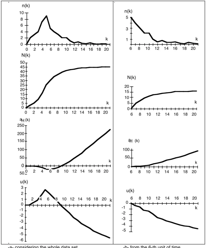
We use hereafter a simple example to illustrate the relationship between these features and the Laplace factor. Figure 4-a gives the failure intensity, the cumulative number of failures, N(k), the curve corresponding to the difference of areas between the chord joining the origin and the current cumulative number of failures and the curve plotting N(k), -aH(k), and the Laplace factor, u(k).

Considering the whole data set (Figure 4-a) leads to the following comments: i) aH(t) is negative until point 9 indicating superadditivity and hence reliability decrease until this point, and ii) the sign of the Laplace factor follows the sign of -aH(t). If we consider now the data set from a point where the function is still superadditive and the Laplace factor is positive, point 6 for example, and plot the same measures in Figure 4-b, the results of this time origin change are: i) aH(t) is positive for each point showing reliability growth over [6, 19], and ii) the Laplace factor becomes negative.

In conclusion, and more generally, changes of the time origin affect in the same manner the subadditive property and the Laplace factor. However, the change in the origin does not result in a simple translation of the curve representing the Laplace factor in all situations: removal of a sub-set of failure data usually amplifies the variations of the Laplace factor due to the presence of the denominator (relation (8)).

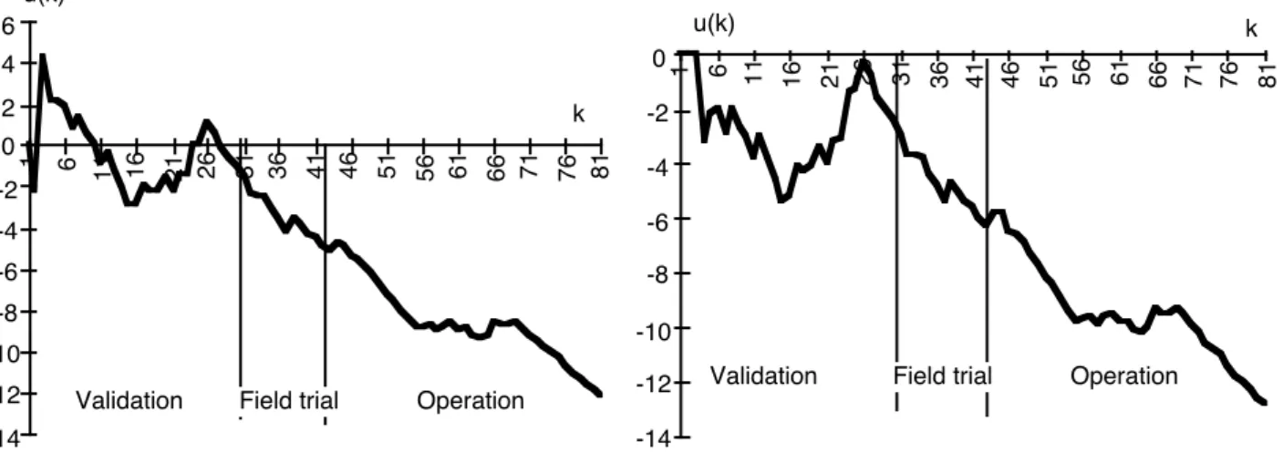
What precedes is illustrated in Figures 5 on a real situation corresponding to experimental data, where the data are relative to the TROPICO-R switching system studied in [11].

Figure 5-a gives the Laplace factor for the whole data set from validation to operation. At the beginning of the validation, reliability decrease took place, as a result of the occurrence of 28 failures during the third unit of time whereas only 8 failures occurred during the first two time units and 24 during the next two time units. This situation is usual during validation: reliability decrease is due to the activation of a great number of faults at the beginning. Applying the Laplace test without the data belonging to the two first units of time leads to reliability growth on average from unit time 3 (figure 5-b). Even though we have removed only two data items, comparison of figures 5-a and 5-b confirms the previous points: i) amplification of the variation of the Laplace factor and ii) conservation of the trend change.

0 2 4 6 8 10 n(k) k 0 5 10 15 20 25 30 35 40 45 50 0 2 4 6 8 10 12 14 16 18 20 N(k) k 50 50 100 150 250 200 k aH (k) -6 -5 -4 -3 -2 -1 0 1 2 3 2 4 6 8 10 12 14 16 18 20 u(k) k 0 2 4 6 8 10 12 14 16 18 20 0 0 2 4 6 8 10 12 14 16 18 20 1 3 5 6 8 10 12 14 16 18 20 n(k) k 0 5 10 15 20 N(k) k 0 50 100 k aH (k) u(k) k -5 -4 -3 -2 -1 0 6 8 10 12 14 16 18 20 6 8 10 12 14 16 18 20 6 8 10 12 14 16 18 20

-a- considering the whole data set -b- from the 6-th unit of time

Figure 4: Subadditive property and Laplace factor

From a pragmatic viewpoint, i.e. using the Laplace factor as a trend indicator rather than a conventional statistical test, the above considerations and the link derived between the Laplace factor and the subadditive property enable reliability growth on average and local trend change to be defined. The denominator of the Laplace factor acts as a norming factor allowing reduction of the range of variation of aH(k). From what precedes — and due to the fact that the Laplace test is already well known and quite used [2, 4] — in real situations, we will use mainly the Laplace test to analyze the trend considering the sign of its factor as well as the evolution of this factor with time as it enables both local trend change and trend on average to be identified "at a glance".

-14 -12 -10 -8 -6 -4 -2 0 2 4 6 1 6 _{11 16 21 26 31 36 41 46 51 56 61 66 71 76 81} u(k) k

Validation Field trial Operation

k -14 -12 -10 -8 -6 -4 -2 0 1 6 _{11 16 21 26 31 36 41 46 51 56 61 66 71 76 81} u(k)

Validation Field trial Operation

-a- considering the whole data set -b- without considering the first two units of time

Figure 5: Laplace factor for the TROPICO-R

3.3. Typical results that can be drawn from trend analyses

Trend analyses are of great help in appreciating the efficiency of test activities and controlling their progress. They help considerably the software development follow up. Indeed graphical tests are very often used in the industrial field [6, 8, 19, 20] (even though they are called differently, such as descriptive statistics or control charts). It is worth noting that the role of trend tests is only to

draw attention to problems that might otherwise not be noticed until too late, and to accelerate

finding of a solution. Trend tests cannot replace the interpretation of someone who knows the software that the data is issued from, as well as the development process and the user environment. In the following, three typical situations are outlined.

Reliability decrease at the beginning of a new activity like i) new life cycle phase, ii) change in

the test sets within the same phase, iii) adding of new users or iv) activating the system in a different profile of use, etc., is generally expected and is considered as a normal situation. Reliability decrease may also result from regression faults. Trend tests allow this kind of behavior to be noticed. If the duration of the period of decrease seems long, one has to pay attention and, in some situations, if it keeps decreasing this can point out some problems within the software: the analysis of the reasons of this decrease as well as the nature of the activated faults is of prime importance in such situations. This type of analysis may help in the decision to re-examine the corresponding piece of software.

Reliability growth after reliability decrease is usually welcomed since it indicates that, after

first faults removal, the corresponding activity reveals less and less faults. When calendar time is used, mainly in operational life, sudden reliability growth may result from a period of time during which the system is less used or is not used at all; it may also result from the fact that some failures are not recorded. When such a situation is noticed, one has to be very careful and, more important, an examination of the reasons of this sudden increase is essential.

Stable reliability with almost no failures indicates that the corresponding activity has reached a

"saturation": application of the corresponding tests set does not reveal new faults, or the corrective actions performed are of no perceptible effect on reliability. One has either to stop testing or to introduce new sets of tests or to proceed to the next phase. More generally, it is recommended to continue to apply a test set as long as it exhibits reliability growth and to stop its application when stable reliability is reached. As a consequence, in real situations, the fact that stable reliability is not reached may lead the validation team (as well as the manager) to take the decision to continue testing before software delivery since it will be more efficient to continue testing and removing faults.

Finally, trend analyses may be of great help for reliability growth models to give better estimations since they can be applied to data displaying trend in accordance with their assumptions rather than blindly. Applying blindly reliability growth models may lead to non realistic results when the trend displayed by the data differs from the one assumed by the model. Failure data can be partitioned according to the trend:

• in case of reliability growth, most of the existing reliability growth models can be applied, • in case of reliability decrease, only models with an increasing failure intensity can be applied, • when the failure data exhibit reliability decrease followed by reliability growth, an S-Shaped

model [18, 21] can be applied,

• when stable reliability is noticed, a constant failure intensity model can be applied (HPP model): reliability growth models are in fact not needed.

4. Application to real systems

This section is intended to illustrate the type of results that can be issued from trend analysis during the development and operational phase, as well as for reliability growth models application. Since the previous section showed how the relationship between the subadditive property and the Laplace factor allows the identification of local trend changes by the Laplace factor, we will use mainly the latter. The aim of this section is just to illustrate some of the points introduced in the previous section and not to make detailed analyses of the considered data sets.

Three different systems are considered: i) the first one corresponds to system SS4 published in [17], called system A hereafter, ii) the second, corresponds to system S27 (referred to as system B) published also in [17], and iii) the last one corresponds to an electronic switching system (referred to as system C) which has been observed during validation and a part of operational life [13]. For each of them, we will give the results of trend analysis and comment on the kind of reliability growth models that could be used.

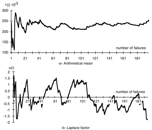
4.1. System A

Failure data gathered on System A correspond to operational life. Application of the arithmetical mean test in figure 6-a shows that the mean time to failure is almost constant: it is about 230 000 units of time. The corresponding Laplace factor displayed in Figure 6-b oscillates between -2 and +2 indicating also stable reliability for a significance level of 5%. In this case, a constant failure rate (i.e., HPP model) is well adapted to model the software behavior and is of simpler application than a reliability growth model. This result is not surprising since the software was not maintained (no fault correction). This is an example of a situation where the classical Laplace test is applicable and sufficient to analyze the trend at a glance (since there are no local trend changes). 100 150 200 250 300 1 21 41 61 81 101 121 141 161 181 number of failures τ(i) 10-3

-a- Arithmetical mean

u(i) -2 -1.5 -1 -0.5 0 0.5 1 1.5 2 1 21 41 61 81 101 121 141 161 181 number of failures -b- Laplace factor

Figure 6 - Trend tests for system A

4.2. System B

System B is an example of systems which exhibit two phases of stable reliability; transition between them took place about failures 23-24 (figure 7). This system was under test and one has to look for the reasons of this sudden change and to see why no reliability growth took place. It was not possible from the published data to identify the reasons of this behavior. In this case, data may be

partitioned into two subsets each of them being modeled by a constant failure rate. Figures 7-a and 7-b illustrate the link between a graphical test (the mean of the inter-failure times) and the Laplace factor: the discontinuity in software behavior is pointed out by both of them.

u(i) number of failures -6 -5 -4 -3 -2 -1 0 1 2 1 5 9 13 17 21 25 29 33 37 41 number of failures 0 20 40 50 80 100 120 1 5 9 13 17 21 25 29 33 37 41 τ (i) 10-3

-a- Laplace factor -b- Arithmetical mean

Figure 7: Trend tests for system B

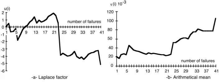
4.3. System C

System C displayed reliability decrease during the validation, reliability growth took place only during operational life as indicated in figure 8-a. This is confirmed by figure 8-b where the Laplace test for operational life is applied to the data collected during operation only. It can also be seen that some reliability fluctuations took place around unit time 15, this fluctuation is due to the introduction of new users. Clearly, not any reliability growth model is applicable during validation. However, an S-Shaped model can be applied to the whole data set and any reliability growth model to operational data (from unit time 9) as carried out in [13]. This is an example of situation where the classical Laplace test does not help in detecting the local trend change around point 9. The only information available from the classical test is that reliability growth took place from point 18 which is indeed so far from the real situation.

-8 -6 -4 -2 0 2 4 u(k) Unit of time Validation Operation 6 2 4 6 8 10 12 14 16 18 20 22 24 26 28 30 32 -8 -6 -4 -2 0 2 4 6 2 4 6 8 Validation Operation Unit of time u(k) 10 12 14 16 18 20 22 24 26 28 3032

-a- For the whole data set -b- For each phase separately

5. Conclusion

In this paper, we have characterized reliability growth and derived a graphical interpretation of the subadditive property and we have shown the equivalence between this property and the Laplace factor allowing thus the Laplace factor to identify local trend changes as well. We have shown i) that trend analyses constitute a major tool during the software development process and ii) how the results can guide the project manager to control the progress of the development activities and even to take the decision to re-examine the software for specific situations. Trend analyses are also really helpful when reliability evaluation is needed. They allow periods of times of reliability growth and reliability decrease to be identified in order to apply reliability growth models to data exhibiting trend in accordance with their modeling assumptions. Trend tests and reliability growth models are part of a global method for software reliability analysis and evaluation which is presented in [13] and which has been applied successfully to data collected on real systems [10, 11, 13].

Acknowledgments

We wish to thank Mohamed Kaâniche and Sylvain Metge from LAAS-CNRS for their helpful comments when reading earlier versions of the paper.

References

[1] E.N.Adams, "Optimizing preventive service of software products", IBM J. of Research and

Development, vol. 28, no. 1, Jan. 1984, pp. 2-14.

[2] H. Ascher and H. Feingold. “Application of Laplace's Test to Repairable Systems Reliability,” in 1st International Conference on Reliability and Maintainability, pp. 254-258, Paris, 1978.

[3] H.Ascher, H.Feingold, Repairable systems reliability: modeling, inference, misconceptions

and their causes, Lecture notes in statistics, Vol. 7, 1984.

[4] D.R.Cox, P.A.W.Lewis, The statistical analysis of series of events, London, Chapman & Hall, 1966.

[5] O.Gaudoin, "Statistical tools for software reliability evaluation", Ph.D. thesis, Joseph Fournier Univ. Grenoble I, Dec. 1990, in French.

[6] M.E.Graden, P.S.Horsley, "The effects of software inspections on a major telecommunica-tions project", AT&T Technical Journal, Vol. 65, Issue 3, 1986, pp 32-40.

[7] B.V.Gnedenko, Yu.K.Belyayev, A.D.Solovyev, Mathematical methods of reliability theory, Academic press, 1969.

[8] R.B.Grady, D.R.Caswell, Software metrics: establishing a company-wide program, Hewlett Packard Company, Prentice Hall, Inc., 1987.

[9] M.Hollander, F.Proschan, "A test for superadditivity for the mean value function of a Non Homogeneous Poisson Process", Stoch. Proc. and their appli. vol. 2, 1974, pp. 195-209.

[10] K.Kanoun, T.Sabourin, "Software dependability of a telephone switching system", Proc. 17th

IEEE Int. Symp. on Fault-Tolerant Comp. (FTCS-17), Pittsburgh, July, 1987, pp. 236-241.

[11] K.Kanoun, M.Bastos Martini, J.Moreira De Souza, "A method for software reliability analysis and prediction — application to the TROPICO-R switching System", IEEE

Transactions on Software Engineering, April 1991, pp. 334-344.

[12] K.Kanoun, J.C.Laprie, "The role of trend analysis in software development and validation", Proc. of Safecomp'91, Trondheim, Norway, 30 Oct. - 1 Nov. 1991, pp. 169-174.

[13] K.Kanoun, M.Kaâniche, J.C.Laprie, "Experience in software reliability: from data collection to quantitative evaluation", Proc. Fourth International Symposium on Software Reliability

Engineering, (ISSRE'93), Denver, Colorado, November 1993, pp. 234-246.

[14] G.Q.Kenney, M.A.Vouk, "Measuring the Field Quality of Wide-Distributed Commercial Software", Proc. of the Third International Symposium on Software Reliability Engineering, ISSRE'92, Research Triangle Park, North Carolina, October 1992, pp. 351-357.

[15] J.C.Laprie, Dependability: basic concepts and terminology, Dependable Computing and Fault-Tolerant Systems, Vol. 5, J.-C. Laprie Editor, Springer Verlag, Wien, New York, 1992. [16] B.Littlewood, "How To Measure Software Reliability and How Not To", IEEE Transactions

on Reliability, vol. R-28, no. 2, June 1979, pp. 103-110.

[17] J.D.Musa, "Software reliability data", Data and Analysis Centre for Software Rome Air Development Centre (RADC) Rome, NY, 1979.

[18] M. Ohba, "Software reliability analysis models", IBM J. of Research and Development, vol. 21, no. 4, July 1984, pp. 428-443.

[19] N.Ross, "The collection and use of data for monitoring software projects", Measurement for

software control and assurance, Edited by B.A.Kitchenham and B.Littlewood, Elsevier

Applied Science, London and New York, 1989, pp. 125-154.

[20] V.Valette, "An environment for software reliability evaluation", Proc. of Software

Engineering & its Applications, Toulouse, France, Dec. 1988, pp. 879-897.

[21] S.Yamada, "Software quality / reliability measurement and assessment: software reliability growth models and data analysis", J. Information Proc. vol. 14, no. 3, 1991, pp. 254-266.