HAL Id: hal-01917877
https://hal.archives-ouvertes.fr/hal-01917877
Submitted on 9 Nov 2018
HAL is a multi-disciplinary open access
archive for the deposit and dissemination of
sci-entific research documents, whether they are
pub-lished or not. The documents may come from
teaching and research institutions in France or
abroad, or from public or private research centers.
L’archive ouverte pluridisciplinaire HAL, est
destinée au dépôt et à la diffusion de documents
scientifiques de niveau recherche, publiés ou non,
émanant des établissements d’enseignement et de
recherche français ou étrangers, des laboratoires
publics ou privés.
Hybrid Modeling Method of Magnetic Field of Axial
Flux Permanent Magnet Machine
Théo Carpi, Yvan Lefèvre, Carole Hénaux
To cite this version:
Théo Carpi, Yvan Lefèvre, Carole Hénaux. Hybrid Modeling Method of Magnetic Field of Axial Flux
Permanent Magnet Machine. 2018 XIII International Conference on Electrical Machines (ICEM), Sep
2018, Alexandropuli, Greece. pp.766-772. �hal-01917877�
OATAO is an open access repository that collects the work of Toulouse
researchers and makes it freely available over the web where possible
Any correspondence concerning this service should be sent
to the repository administrator:
tech-oatao@listes-diff.inp-toulouse.fr
This is an author’s version published in:
http://oatao.univ-toulouse.fr/20819
To cite this version:
Carpi, Théo and Lefèvre, Yvan and Henaux, Carole Hybrid
Modeling Method of Magnetic Field of Axial Flux Permanent
Magnet Machine. (2018) In: 2018 XIII International
Conference on Electrical Machines (ICEM), 3-6 September
2018 (Alexandropuli, Greece)
Official URL:
https://doi.org/10.1109/ICELMACH.2018.8506756
Open Archive Toulouse Archive Ouverte
ΦAbstract – A hybrid analytical-numerical method to predict the no-load magnetic flux density in an axial flux permanent magnet (AFPM) machine is presented in this paper. It involves the method of separation of variables. This leads to express the magnetic scalar potential (MSP) by a series where each term is the product of three functions. The function depending on the radial coordinate is determined by means of a 1-D finite difference method (FD) instead of using Bessel functions. The functions depending on the axial and azimuthal coordinates are described by Fourier series. The results obtained by this method are compared to the results obtained by 3D finite element analysis (FEA).
Index Terms—Axial flux, finite difference method, Fourier
series, magnetic scalar potential, permanent magnet (PM), separation of variables.
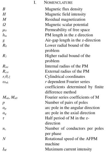
I. NOMENCLATURE
B Magnetic flux density
H Magnetic field intensity
M Residual magnetization
Ω Magnetic scalar potential
µ0 Permeability of free space
hm PM length in the z direction
g Air-gap length in the z-direction
R0 Lower radial bound of the
problem
R1 Higher radial bound of the
problem
Rint Internal radius of the PM
Rext External radius of the PM
r,θ,z Cylindrical coordinates
ωnk r dependent Fourier series
coefficients determined by finite difference method
Mnk, Mn0 Fourier series coefficients of M
p Number of pairs of poles
αp arc pole in the angular direction
αq arc pole in the axial direction
τ Half period of M in the z- direction
nc Number of conductors per poles
per phase
N Rotational speed of the AFPM machine
IM Maximum current intensity
ΦT. Carpi, Y. Lefevre and C. Henaux are with Laboratoire Plasma et
Conversion d’Energie (LAPLACE), University of Toulouse, CNRS, 31000 Toulouse, France (email: {tcarpi, lefevre, henaux}@laplace.univ-tlse.fr).
II. INTRODUCTION
HE growing interest in axial-flux permanent magnet (AFPM) machines, due to its good torque-to-weight ratio [1], requires fast magnetic flux prediction for sizing or optimization studies for example.
Analytical modeling of PM machines by the separation of variable technique provides fast and good results compared to finite elements method (FEM). The method of separation of variables is suitable for 2D problems [2]-[4] but becomes more complicated when applied to a 3D problem such as an AFPM machine due to a second separation constant to handle. A quasi-3D model based on a 2-D resolution at the mean radius is proposed in [5]. [6] makes the 3-D solution possible by using a Fourier integral in the radial coordinate while [7] uses a two variable Fourier series in angular and axial coordinate by means of the image method. Apart from the separation of variable technique, an analytical solution based on the integral transform method is proposed in [8] while [9] uses free-space Green’s function method. Nevertheless, these solutions involve Bessel functions which increase the complexity of the problem and calculation time. The purpose of this paper is to present an alternative technique to model the open-circuit magnetic flux density in an AFPM machine. It consists in a hybrid approach, partially analytical, partially obtained by finite difference (FD) method. The problem is first described analytically with the help of Fourier series and separation of variables to finally apply the FD method to the radial coordinate which is the most complicated to handle.
III. PROBLEM DEFINITION
A. Geometry and Assumptions
A four pairs of poles AFPM machines is considered with axially alternatively magnetized surface-mounted permanent magnets as shown in Fig. 1.
Fig. 1. 3-D representation of a pair of poles of the AFPM machine.
Hybrid Modeling Method of Magnetic Field of
Axial Flux Permanent Magnet Machine
T. Carpi, Y. Lefevre, C. Henaux
To simplify the problem, the following assumptions are made:
- Because of the air-space between the magnets, we assume that the permeability in the magnets and the air is the same and equal to µ0. Therefore, magnetic constitutive laws
give us the relation between magnetic field and magnetic flux density:
(
)
( )
10 H M
B = μ +
- Back-irons have infinite permeability so the boundary conditions at the planes z = 0 and z = hm + g are taken as
Neumann boundary.
- The problem is limited in the radial direction with parallel flux boundary conditions on cylinders at r = R0 and r
= R1.
Fig. 2. Periodical extension in the z direction in a cylindrical cut-view of the AFPM machine.
Fig. 3. Angular (a) and axial (b) dependency of the magnetization.
B. Fourier series Magnetization Description
Homogeneity of permeability inside and between the magnets allows describing the residual magnetization M as a Fourier series in the angular coordinate. To reduce even more the number of regions and thus simplify the problem, Neumann boundary conditions can be replaced by a periodical extension of the residual magnetization in the z-direction by virtue of the method of images [7] as shown in Fig. 2.
Thus, in the cylindrical coordinate system, M has only a component in the axial direction and can be expressed as a Fourier series of two variables θ and z:
( )
( )
( )
2 5 , 3 , 1 cos 0 5 , 3 , 1 cos 1 cos
∞ = + ∞ = ∞ = = n np n M n z k k np nk M z M θ τ π θwhere p is the number of pairs of poles and τ is the half period of the signal in the z-direction (τ = hm + g) and Mnk
and Mn0 are the Fourier series coefficients. They are
calculated from the waveforms of Mz(z) and Mz(θ) shown in
Fig. 3.
( )
( )
4 2 sin 4 0 3 sin 2 sin 2 8
= = p n n M q n M q k p n nk M nk M α π π α α π α π πwhere αp and αq are the arc pole coefficients in the angular
direction and the axial direction respectively.
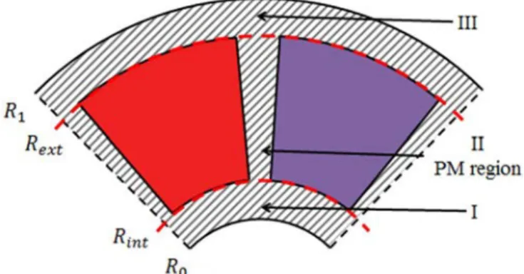
Therefore, there are three regions to be considered separated by cylindrical surfaces at r = Rint and r = Rext. Air
regions I (R0 ≥ r ≥ Rint ) and III (Rext ≥ r ≥ R1), and the PM
region II (Rint ≥ r ≥ Rext) are shown in Fig. 4.
Fig. 4. Representation of the different regions considered in the problem.
In this problem, a one-sided AFPM machine is considered. However, the image method, illustrated in Fig. 1, demonstrates that the technique presented in this paper can be applied to a double-sided AFPM machine as the Fourier series description allow to compute the solution for z > hm +
g. Thus, the same description can be applied for a double
sided AFPM machine as shown in Fig. 5. The winding distribution is, as in the one-sided AFPM machine, placed at the plane z > hm + g.
Fig. 5. Periodical extension in the z-direction of a double-sided AFPM machine represented in a cylindrical cut-view.
IV. SOLUTION OF THE PROBLEM
C. Separation of variables
The problem is now described so that the separation of variables is more convenient to apply. Indeed, the definition of the three regions implies two boundary conditions at r =
R0 and r = R1 and two interface conditions at r = Rint and r =
Rext.
This open circuit study enables to write Maxwell’s equations as follow:
( )
5
Ω − = grad H( )
6
0 = B divCombining (1), (5) and (6) yields to the partial differential equation:
( )
7
M div = ΔΩThe divergence of M is expressed, in cylindrical coordinates as:
( )
8 1 z z M M r r r M r r M M div ∂ ∂ + ∂ ∂ + ∂ ∂ + = θθM has only an axial component, therefore:
( )
( )
9
5 , 3 , 1 sin 1 cos .
∞
= ∞ = − = ∂ ∂ n z k k np nk M k z z M τ π θ τ πThen, (7) become, for each region considered:
( )
( )
( )
12 11 10 0 2 2 2 2 2 1 1 2 2 2 2 2 2 2 1 1 2 2 0 2 2 2 2 2 1 1 2 2 = ∂ Ω ∂ + ∂ Ω ∂ + ∂ Ω ∂ + ∂ Ω ∂ ∂ ∂ = ∂ Ω ∂ + ∂ Ω ∂ + ∂ Ω ∂ + ∂ Ω ∂ = ∂ Ω ∂ + ∂ Ω ∂ + ∂ Ω ∂ + ∂ Ω ∂ z III III r r III r r III z z M z II II r r II r r II z I I r r I r r I θ θ θUsing the separation of variables [10], Ω is considered to be the product of three functions each dependent on only one coordinate of the cylindrical coordinate system:
( )
13
)
(
.
)
(
.
)
(
r
g
h
z
f
θ
=
Ω
Incorporating (13) in the Laplacian leads to three separated ordinary differential equations for f, g and h:
( )
( )
( )
− = ∂ ∂ − = ∂ ∂ = + − ∂ ∂ + ∂ ∂ 16 2 2 2 2 15 2 1 2 2 14 0 2 2 2 2 1 1 2 2 h z h g g f r r f r r f α α θ α αα12 and α22 are the separation constants and can be chosen
either positive or negative. Their sign is chosen in order to fit the form of the sources, indeed (15) and (16) are solved with a linear combination of sines and cosines function. Equation (14) is a Bessel differential equation and gives modified
Bessel functions of first and second kind of order α1 as the
solution [11]:
( )
( )
( )
( )
( )
( )
( )
( )
( )
19 18 17 2 sin . 2 cos . : 1 sin . 1 cos . : 2 1 . 2 1 . : z F z E z h D C g r K B r I A r f α α θ α θ α θ α α α α + → + → + →where A, B, C, D, E and F are arbitrary coefficients.
Handling Bessel functions add to the complexity of the problem and involve additional numerical functions to approach them. The method presented here proposes solving the r dependence differential equation by finite difference method which is easy to implement and might produce a solution close enough to FEM method to be considered as a useful alternative model. It may provide a fast and precise model of the magnetic flux density produced by the permanent magnets compared to analytical models proposed in [6] and [7] in which the expressions of the air-gap magnetic flux density are relatively complex. Thus, the solution f including Bessel functions is not considered, and an alternative solution involving finite difference method is presented.
D. Finite Difference Method
Due to the description of the magnetization given in (2) and the equations in the different regions (10), (11) and (12), the solution can be assumed with the same form as the second member of (11) also described in (9). Moreover, α1 and α2 are
identified to np and kπ/τ respectively and discretize the values of α1 and α2.
With the help of the two variable Fourier series description and the principle of superposition, the general solution is written as follow:
(
)
( ) ( )
( )
20
5 , 3 , 1 sin 1 cos , ,
∞ = ∞ = = Ω n z k k np r nk z r τ π θ ω θwhere ωnk are the r dependent Fourier series coefficients to
be determined by FD method. An additional term ωn0 should
be added to the solution (20) but will not be considered as it will vanish from the Bz component of the magnetic flux
density according to (21).
( )
21
0
+ ∂ Ω ∂ − = z M z z B μCombining (20) and the partial differential equations in regions I, II and III yields to the following ordinary differential equations over the r dependent Fourier series coefficient in each region:
( )
22 0 2 2 2 2 2 2 1 2 2 = + − + I nk k r p n dr I nk d r dr I nk dω
τ π ω ω( )
23 2 2 2 2 2 2 1 2 2 − = + − + τ π τ π ω ωω
k nk M k r p n dr II nk d r dr II nk d II nk( )
24 0 2 2 2 2 2 2 1 2 2 = + − + III nk k r p n dr III nk d r dr III nk dω
τ π ω ωmethod is then applied for R0 ≥ r ≥ R1 and for all couples (n,
k). The discretization of the radius is achieved with a variable
step as shown in Fig. 6.
Fig. 6. Definition of variables used in FD method with a variable step.
The second order Taylor approximation are used to compute the derivatives of ωnk given in (25) and (26).
(
)
( )
25 1 1 1 2 2 2 1 1 2 1 − + − + + − − − − − = i h i h i h i h i u i h i u i h i h i u i h i dr nk dω(
)
(
)
( )
26 1 1 1 1 1 1 2 2 2 − + − + + − − − − − = i h i h i h i h i u i h i u i h i h i u i h i dr nk dωwhere ui represents the value of ωnk for r = ri and hi the
step between ri+1 and ri. Therefore, differential equations
(22), (23) and (24) in each region along with discretization proposed in (25) and (26) yields to three solutions for all radius between R0 > r >Rint ,Rint > r > Rext and Rext > r > R1.
The problem formulated by (22), (23) and (24) after discretization leads to the following system in each region:
)
27
(
. . .
= = = III nk B III nk v III nk A II nk B II nk v II nk A I nk B I nk v I nk Awhere Ank is the matrix of rank (n, k) of the coefficients of the
components of the vector vnk (i) = ui and Bnk is the vector
whose components are the second member of each differential equation. The formulation (27) is now completed by boundary and interface conditions at r = R0, r = Rint, r =
Rext and r = R1. ) 31 ( 0 ) 30 ( ) 29 ( ) 28 ( 0 1 int 0 = = = = = = = = III r III r II r ext II r I r I r H R r H H R r H H R r H R r
Traduced in MSP and then in DF it yields to:
) 35 ( 0 ) 34 ( ) 33 ( ) 32 ( 0 1 1 1 1 1 1 1 1 1 int 1 1 0 = − = − = − = − = − = = − = − − + − − + − − − − i III i III i i III i III i i II i II i ext i II i II i i I i I i i I i I i h u u R r h u u h u u R r h u u h u u R r h u u R r
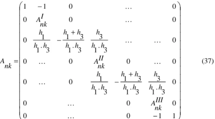
The problem can now be formulated generally by the following matrix equation:
) 36 ( . nk B nk v nk A = with ) 37 ( 1 1 0 0 0 0 0 0 3 . 1 3 3 . 1 3 1 3 . 1 1 0 0 0 0 0 0 0 3 . 1 3 3 . 1 3 1 3 . 1 1 0 0 0 0 0 0 1 1 − + − + − − = III nk A h h h h h h h h h h II nk A h h h h h h h h h h I nk A nk A
and Bnk(i) = Mnk in the region II and 0 in region I and III. To
compute the final solution Bz (r,θ,z), the solution of (36),
constitutive law (21) and the general form of the solution (20) are combined:
( )
( )
( )
38
5 , 3 , 1 cos 1 . cos 0 , ,
+ ∞ = ∞ = − = z M n z k k k np nk v z r z B τ π τ π θ μ θThe axial magnetic flux is discretized in r and then can be computed for any value of θ and z.
E. Electromotive Force and Torque
The main advantage of this technique is that all information of the AFPM such as back electromotive force (emf) and torque can be deduced from the z component of the magnetic flux density. Furthermore, it can be computed for any winding distribution.
In an AFPM machine, conductors are placed on a radial line. Therefore, to be as accurate as possible, meshing of the problem has to be discretized radially and angularly in order to get each point on a radial line corresponding to a conductor. The conductors are considered to be radial filaments placed at the plane z = hm + g between radius Rint
and Rext.
The back emf is the rate of change of the magnetic flux density. Thus, the elementary back emf generated over a single conductor is computed according to the following expression:
( )
( )
39
int , , . . dr ext R R r Bz r hm g elem e
+ = ω θ θwhere ω is the angular speed of the AFPM machine and θ the relative angular position of the stator compared to the rotor. The total back emf is then deduced from this elementary calculation depending on the winding distribution. The winding distribution considered is a simple three phase winding and is shown in Fig. 7.
Then, the total back emf is deduced from (21):
( )
(
( ))
( )
40
1 ) ( 1 . θ θ θ eR F e c n p tot e = −where etot is the total back emf over the phase one, eF1 and eR2
are the elementary back emf generated respectively over the forward conductor and the backward conductor of the phase one, nc is the number of conductors per pole per phase and p
is the number of pairs of poles of the AFPM machine.
The same way, the elementary torque is computed over a single conductor with unitary current and unitary number of conductors per pole per phase in order to apply it over any kind of winding distribution:
( )
( )
41
int , , . dr ext R R rBz r hm g elem T
+ = θ θPhases are powered by sinusoidal currents of magnitude
IM, the total torque is computed at the time when the current
of the phase 1, 2 and 3 are respectively equal to IM, -IM/2 and
-IM/2, in other words, at maximum torque. The torque per
phase is then:
( )
. .(
)
( )
42
Rk T k I Fk T k I c n p k T θ = −where Ik is the current of the phase k, TFk and TRk are
respectively the elementary torques exerted on the forward conductor of the phase k and on the backward conductor of the phase k. Total torque is then deduced by summation.
V. STUDIED AXIAL FLUX MACHINE
The AFPM considered here is slotless and its parameters are given in Table 1. The complete view of the machine is shown in Fig 8. The conductors are considered as filaments and each color represent one phase.
TABLEI
PARAMETERS OF THE AFPMMACHINE
Parameter Value Br 1.29 T hm 5 mm g 6 mm R0 10 mm R1 32 mm Rint 13.5 mm Rext 28.5 mm p 4 αp 0,8 N 1500 tr/min nc 12 IM 2 A
Some experiments are currently being performed on the same kind of machine. These experimental results will be presented in the final article to validate the model.
The model is thus applied to a pair of poles of this AFPM machine. The torque and back emf are deduced from the axial component of the magnetic flux density Bz (39) according to
(40)-(42).
Fig. 8. Complete view of the AFPM considered in the study.
VI. FINITE ELEMENT COMPARISON
To confirm the validity of the solution previously presented, a finite element analysis based on scalar potential formulation is performed on ANSYS/Emag 3D [12].
The conditions of both calculation methods have to be the same, therefore, the same boundary conditions are set: normal flux at planes z = 0 and z = hm + g and parallel flux at
cylindrical planes r = R0 and r = R1. Also, the permeability is
set to µ0 for both magnets region and air region.
To perform a complete comparison, both computation methods will be achieved on a radial line, for z = hm + g/2
and θ = 0, a circumferential line at r = Rint + 0.8.(Rext-Rint)
and z = hm + g/2 and an axial line at r = Rint + 0.8.(Rext-Rint)
and θ = 0. Thus, the comparison is made on three plots that will show the validity of the model in accordance with r, θ and z independently.
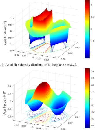
Fig. 9 and Fig. 10 show the air gap field generated by three poles respectively in the magnets at the plane z = hm/2 and in
the air gap at the plane z = hm + g/2.
Fig. 9. Axial flux density distribution at the plane z = hm/2.
The magnetization is a square wave and therefore requires many harmonics to reach the waveform shown in Fig. 3. Even if the waveforms from Fig. 11 are unsquared, the expression of axial magnetic flux density involves Mz
expression (modulated by µ0) and thus may alter the quality
of the signal. The axial magnetic flux density as a function of
z is the most influenced by this feature. Indeed, considering
both magnets and air-gap region, the root mean square error
(a)
(b)
(c)
Fig. 11. Axial flux density as a function of axial coordinate (a), angular coordinate (b) and radial coordinate (c) by hybrid analytical-FD method and FEM.
goes from 6% for 11 harmonics and globally decrease until 1.5% for 101 harmonics but is not monotonous. This is due to the square wave of the axial magnetic flux density in the magnets region which induces a large error for a low number of harmonics.
Thus, most of the error comes from the magnets region. Considering only the air-gap region, which is of our interest, the error becomes smoother and below 1.5% beyond 16 harmonics as shown in Fig. 12.
Radial and angular dependence are less affected by the quality of the magnetization and the RMS error is about 2% and 1.6% respectively in accordance with radial and angular coordinate.
This method includes several nested loops so the computation time increase exponentially with respect to the number of harmonics and the discretization step. The results presented here are computed for 16 harmonics and 1 894 053 points in the volume considered for a total computation time of nine seconds. Fig. 12 shows that it not necessary to reach a high harmonic order to obtain a reasonable accuracy of the model. Despite the low number of harmonics, the waveforms are smooth and the error is below 2% on each plot.
Fig. 12. Accuracy and computation time in accordance with the number of harmonics.
Back emf and torque waveforms are deduced from the axial component of the magnetic flux density over the plane z
= hm + g as presented in section IV. The computation is made
for both calculation methods for the winding distribution given in Fig. 7 at the moment of maximum torque defined previously, and for all angular position of the rotor compared to the stator. The angular position θ = 0° is set to be the one shown in Fig. 7 and the rotor is rotating counter-clockwise. Fig. 13 and 14 show the back emf and torque waveforms versus angular position.
Both methods are very close; indeed, the RMS error between the hybrid solution and the FEM is 0.70% and 0.46% respectively for the back emf and the torque. This validates the correctness of the hybrid solution. Errors on back emf and torque between the proposed method and the FEM are directly related to the error on Bz but it gives an
additional point of comparison as it is calculated at the plane
Fig. 13. Back emf waveform computed for the given winding distribution depending on the relative angular position of the rotor compared to the stator.
Fig. 14. Total torque waveform computed for the given winding distribution depending on the relative angular position of the rotor compared to the stator.
VII. CONCLUSION
The method proposed here to predict the magnetic flux density in an AFPM machine is an efficient alternative to fully analytical models proposed in [6], [7]. Indeed, the 1-D finite difference method is easy to set up, and the calculation time is more than acceptable for a small number of harmonics. Nevertheless, the magnetization description requires a lot of harmonics and may bring in some additional error but remains reasonable. Finally, the axial component of the magnetic flux density provides access to back emf and torque of the AFPM machine for any kind of winding distribution.
This method can be adapted to all types of magnets distributions and to other kind of problems as long as it can be described by Fourier series and the separation of variables.
VIII. REFERENCES
[1] Aydin, M., Huang, S., Lipo, T.: “Axial flux permanent magnet disc machines: a review”. Proc. of the 2004 SPEEDAM, 2004.
[2] Z. Q. Zhu; D. Howe; E. Bolte; B. Ackermann, "Instantaneous magnetic field distribution in brushless permanent magnet dc motors, part I: Open-circuit field, " IEEE Trans. Magn., pp. 124-135, 1993.
[3] N. Bianchi, "Analytical field computation of a tubular permanent-magnet linear motor", IEEE Trans. Magn, vol. 36, no. 5, pp. 3798-3801, Sep. 2000.
[4] A. Rahideh, T. Korakianitis, "Analytical armature reaction field distribution of slotless brushless machines with inset permanent magnets", IEEE Trans. Magn., vol. 48, no. 7, pp. 2178-2191, Jul. 2012. [5] J. Azzouzi, G. Barakat, B. Dakyo, "Quasi-3-D analytical modeling of the magnetic field of an axial flux permanent-magnet synchronous machine", IEEE Trans. Energy Convers., vol. 20, no. 4, pp. 746-752, Dec. 2005.
[6] Y. Huang, B. Ge, J. Dong, H. Lin, J. Zhu, Y. Guo, "3-D analytical modeling of no-load magnetic field of ironless axial flux permanent magnet machine", IEEE Trans. Magn., vol. 48, no. 11, pp. 2929-2932, Nov. 2012.
[7] Ping Jin, Yue Yuan, Miyi Jin et al., "3-D analytical magnetic field analysis of axial flux permanent-magnet machine [J]", IEEE Trans. Magn, vol. 50, no. 11, pp. 3504-3507, 2014.
[8] Y. N. Zhilichev, “Three-dimensional analytic model of permanent magnet axial flux machine”, IEEE Trans. Magn., vol. 34, no. 6,pp. 3897–3901, Nov. 1998.
[9] E. P. Furlani, M. A. Knewtso, "A three-dimensional field solution for permanent-magnet axial-field motor", IEEE Trans. Magn., vol. 33, no. 3, pp. 2322-2325, May 1997.
[10] R. Haberman, "Applied Partial Differential Equations with Fourier Series and Boundary Value Problems", 5th edition, Pearson, 2013. [11] Moon, P., Spencer, D.E., 1961. "Field theory handbook including
coordinate systems, differential equations, and their solutions". 236, Berlin, 1988.
[12] ANSYS Mechanical APDL Low Frequency Electromagnetic Analysis 215 Guide. Release 17.2, document, Aug. 2016.
IX. BIOGRAPHIES
Theo Carpi was graduated from ENSEEIHT of Toulouse, France, in
electrical engineering in 2016. He is currently pursuing the Ph.D. degree in electrical engineering at the Laboratoire Plasma et Conversion d’Energie (LAPLACE), Toulouse.
Yvan Lefevre was graduated from ENSEEIHT of Toulouse,
France, in electrical engineering in 1983 and received the Ph.D. degree from the Institut National Polytechnique de Toulouse in 1988. He is currently working as a CNRS Researcher at Laboratoire Plasma et Conversion d’Energie (LAPLACE). His field of interest is the modeling of coupled phenomena in electrical machines in view of their design.
Carole Henaux received the Dipl. Ing. Degree in Electrical
Engineering from ENSEEIHT, Toulouse, France, in 1992 and the PHD degree from the Institut National Polytechnique de Toulouse in 1996. She is now a Lecturer with the Electrical Engineering department of INPT / ENSEEIHT.