Competing risks models of economic behavior : theory and applications to retirement and unemployment

THEORY AND APPLICATIONS TO RETIREMENT AND UNEMPLOYMENT

by

GLENN TETSUMI SUEYOSHI

B.A., Pitzer College (1983)

SUBMITTED IN PARTIAL FULFILLMENT OF THE REQUIREMENTS FOR THE

DEGREE OF

DOCTOR OF PHILOSOPHY at the

MASSACHUSETTS INSTITUTE OF TECHNOLOGY September 1987

0 Glenn Tetsumi Sueyoshi

The author hereby grants to M.I.T. permission to reproduce and to distribute copies of this thesis document in whole or in part.

Signature of Author Department of Economics Certified by V V Certified by_ Accepted

by

Jerry A. Hausman, Thesis Supervisor

James M. Poterba, Thesis Supervisor

Peter Temin Chairperson, Departmental Graduate Committee

Archives

L)

MITLibraries

Document Services

DISCLAIMER OF QUALITY

Due to the

condition of the original

material, there are unavoidable

flaws in this reproduction. We have made every effort possible to

provide you with the best copy available. If you are dissatisfied with

this product and find it unusable, please contact Document Services as

soon as possible.

Thank you.

The Archives copy of this thesis is missing page 94. This is the most

complete version available.

Competing Risks Models of Economic Behavior: Theory and Applications to Retirement and Unemployment

by

Glenn Tetsumi Sueyoshi

Submitted to the Department of Economics on September 1, 1987 in partial fulfillment

of the requirements for the Degree of Doctor of Philosophy

Abs tract

Economists increasingly have become involved in the development and use of statistical models for the analysis of duration data. This thesis consists of three chapters which relate to the specification and application of these models to the study of economic phenomena.

In chapter 1, I analyze the determinants of retirement in a competing risk framework, and find that distinguishing between full and partial retirement is important if one wishes to understand the factors influencing the decision to retire. In particular, the Social Security system affects full and partial retirement probabilitites differentially. Chapter 2 consists of an analysis of the duration of unemployment spells. Using a newly developed data source I find that there is mixed support for a simple search interpretation of spell duration. The evidence suggests that a more general framework is required. In chapter 3, I extend the regression form of the

proportional hazards model to the case where covariates are allowed to vary over time. I demonstrate identification and asymptotic normality of the general estimator for both single and competing risks models.

The results in this thesis address specific questions regarding Social Security and unemployment insurance as well as issues relating to the general use of duration models in explaining economic

phenomena. The framework of analysis used in this thesis should profitably extend to a number of areas of future research.

Thesis Supervisors: Jerry A. Hausman, Professor of Economics

Table of Contents

Acknowledgements. . . . . . . . . . . . . . . . . . . . . . . .

Introduction. . . . . . . . . . . . . . . . . . . . . . . . . .

Chapter 1: Social Security and the Determinants of Full and Partial Retirement: A Competing Risks Analysis Introduction . . . . . . . . . . . . . . . . . . . . 1. Background . . . . . . . . . . . . . . . . . . . 1.1 Social Security. . . . . . . . . . . . . .

1.2 Partial Retirement . . . . . . . . . . . .

1.2.1 The Definition of Retirement. . . .

1.2.2 The Extent of Partial Retirement. .

2. The Existing Literature. . . . . . . . . . . . . 3. Econometric Specification.. ... ..... . . . ..

3.1 Single Risk Estimation . . . . . . . . . . 3.2 Competing Risks Estimation . . . . . . . .

4. Data . . . . . . . . . . . . . . . . . . . . . . 5. Results. . . . . . . . . . . . . . . . . . . . .

5.1 Single Form of Retirement . . . . . . . . 5.1.1. Parametric Baseline Hazard (Weibull 5.1.2. Semi-Parametric Baseline Hazard. . 5.2 Full and Partial Retirement. . . . . . . . 5.2.1. Independent Risks. . . . . . . . . 5.2.2. Correlated Risks . . . . . . . . .

Conclusion . . . . . . . . . . . . . . . . . . . . .

er 2: Unemployment Insurance Benefits and the Duration Unemployment Spells: Evidence from the Survey of

Income and Program Participation

Introduction . . . . . . . . . . . . . . . . . . . . . . . 1. Background . . . . . . . . . . . . . . . . . . . . . . 2. Data Issues. . . . . . . . . . . . . . . . . . . . . . * 10 * 13 . 13 . 20 . 20 . 23 . 31 36 37 43 48 . 53 56 56 61 75 75 84 93 of 95 98 .102 Chapt

3. Results. . . . . . . . . . . . . . . . . . . . . . . . .109

3.1 Descriptive Results. . . . . . . . . . . . . . . .109

3.2 Single Risk Models . . . . . . . . . . . . . . . .128

3.3 Competing Risks Models . . . . . . . . . . . . . .139

4. Conclusion . . . . . . . . . . . . . . . . . . . . . . .152

Chapter 3: Semi-parametric Proportional Hazards Estimation of Single and Competing Risks Models with Time-varying Covariates Introduction . . . . . . . . . . . . . . . . . . . . . . . .154

1. Single Risk Duration Models. . . . . . . . . . . . . . .157

1.1 Specification. . . . . . . . . . . . . . . . . . .157

1.2 Identification, Consistency and Asymptotic Normality. . . . . . . . . . . . . . . . . . . . .163

2. Competing Risks Duration Models. . . . . . . . . . . . .176

2.1 Specification. . . . . . . . . . . . . . . . . . .176

2.2 Identification, Consistency and Asymptotic Normality. . . . . . . . . . . . . . . . . . . . .180 3. Conclusion . . . . . . . . . . . . . . . . . . . . . . .193 Appendix 1. . . . . . . . . . . . . . . .195 Appendix 2. . . . . . . . . . . . . . . . . . . . .198 Appendix 3. . . . . . . . . . . . . . . .201 References. . . . . . . . . . . . . . . . . . . . . . . . .2 . .203

Acknowledgements

I would, as is customary, like to acknowledge the contributions of those without whom this thesis could not possibly have been

completed.

First and foremost, I wish to thank my thesis advisors, Jerry Hausman and James Poterba, for wading through my excessively lengthy prose and providing valuable direction and comments. Perhaps more

importantly, they tolerated my peculiar last-minute working style and I am particularly indebted to them for the rapid turnaround time on my manuscripts. My thanks also go to Aaron Han and Hidehiko Ichimura

for help in clarifying a variety of econometric issues associated with duration models and to Steve Venti for timely provision of the SIPP data.

One of the externalities associated with graduate study at M.I.T. is the value of the contributions that one's colleagues make to the final version of a thesis. Rather than provide a lengthly list of individuals, let me instead gratefully acknowledge the

immense collective contribution of the M.I.T. economics community to this thesis. I am also grateful for the financial support provided by the National Science Foundation and M.I.T. economics department. Having good colleagues who are also good friends is more than one should expect and in that regard, I consider myself quite fortunate. At the risk of offending those excluded, I would particularly like to thank James Dana, Janice Eberly, William

English, Robert Gertner, Hidehiko Ichimura, Gregory Leonard, Pamela Loprest, Raymond McFadden, Anne Maasland, Bradley Reiff, Danny Quah, Christopher Vellturo, and especially Leslie Papke, for making

graduate student life bearable.

Above all, my family deserves a lot of credit for putting up with my particular idiosyncracies for the past 25 years. They were never quite certain what I was doing with my life, but trusted me enough to find my own direction. And lastly, I cannot overstate the

importance of Julie Boyer who has, in inumerable ways and in her inimitable style, been an integral part of the past seven years of my life. Boyer has always been there when needed, and her importance is immeasurable. To my family and Julie, this thesis is respectfully dedicated.

Introduction

Economists increasingly have become involved in the development and use of techniques for the analysis of duration data. Duration, or hazard, models provide a convenient framework for examining

economic phenomena which relate to the length of time before an event occurs. This thesis consists of three chapters which involve the use of hazard models in economics.

The first two chapters are comprised of empirical analyses using semi-parametric techniques for the estimation of competing risks models. In the first chapter, I analyze the factors influencing the number of years to retirement and the form, full or partial, that the intitial retirement takes. The second chapter considers the factors

that affect unemployment spell durations and whether exit is via recall or a new job finding. In the third chapter, I demonstrate identification and asymptotic normality for an estimator which generalizes previous semi-parametric estimators to allow for explanatory variables which change over time. The development of this estimator continues the effort, initiated by others, directed at finding a unified framework for the analysis of duration data.

In chapter 1 I examine the relationship between Social Security and retirement behavior. Empirical analyses of retirement typically assume a single form of retirement. There is evidence, however, that

a substantial proportion of individuals exit from full time work via a partial reduction in work effort. To the extent that behavior differs across retirement type, then single form of retirement models

are likely to convolute the influences of various factors upon the two forms of retirement. If, for example, the receipt of Social Security benefits has differential effects by type of retirement, then the single form model will not accurately capture the impact of benefits upon behavior.

To account for the existence of partial retirement, I use a competing risks model of full and partial retirement to analyze retirement decisions. The individual level data are drawn from a sample of Longitudinal Retirement History Survey individuals. Based upon parameter estimates from this specification, I find evidence that single form of retirement models convolute the influence of variables. Additional Social Security benefits are found to increase the probabilities of retirement differentially across retirement type, encouraging full retirement more than partial retirement. A similar result is observed for increases in benefit levels resulting from additional work which lower the relative probability of partial retirement.

The second chapter addresses the impact of unemployment insurance upon the duration of spells of unemployment. Despite considerable advance in both economic theory and econometric

been handicapped by data limitations which hamper the study of a variety of issues. In this chapter, I consider jointly the issue of the impact of UI benefits upon exit from spells of unemployment and the form in which the exit occurs. The primary contribution of the chapter is the development of a new sample of unemployment spells from the Survey of Income and Program Participation which allows for the estimation of a competing risk model of recall or new job finding and which addresses a number of data problems.

I find that unemployment benefits and the exhaustion of benefits are important factors in influencing hazard rates. There is mixed support in the data for a search model of new job finding. While the overall hazard is estimated to be a decreasing function of duration, the new job hazard for exit from unemployment appears to be

increasing over time, but not monotonically. The relative importance of unemployment insurance in affecting the hazards for recall is a result that is beyond the scope of search models to explain and suggests the need for more general models of unemployment durations. These results, along with the finding of a large number of multiple

spell individuals, indicate that the recent concern with the duration of single spell unemployment is somewhat missplaced.

The final chapter builds upon the previous literature on

semi-parametric hazard models by extending the regression form of the proportional hazards model to time-varying covariates. Recent

estimation methods which do not require functional form restrictions on the form of the baseline hazard. Unfortunately, those techniques based upon the regression form of the likelihood have, to date, been restricted to the special case of covariates which do not vary over

time.

I demonstrate identification and asymptotic normality of the general estimator for single and competing risks models with

time-varying covariates. The proofs borrow heavily from the existing literature on hazard models and discrete choice estimators. In the course of demonstrating the properties of the estimator, I take advantage of and point out the obvious correspondence between the semi-parametric estimation techniques and existing discrete choice models. This correspondence should provide the basis for future research on the estimation of hazard models.

Taken together, the three chapters of this thesis address a broad range of issues relating to the specific application of

duration models to the study of retirement and unemployment, and the general use of these models in explaining a variety of economic issues. The framework of analysis used in this thesis should

Chapter 1

Social Security and the Determinants of Full and Partial Retirement: A Competing

Risks Analysis

Intrxlduction

The Social Security system affects individual intertemporal budget constraints through a complicated combination of taxes and transfers. Despite the complexity of the task, several researchers have been able to document the most important of these effects,

tracing the impact of a variety of Social Security rules upon the budget constraint of a given individual. However, the labor supply effects of changes in these constraints are less well understood. Despite a number of attempts at quantification, important unanswered

questions remain regarding the relationship between the Social

Security system and retirement behavior. In this chapter I consider a particular variant of this theme--the interrelated questions of what factors influence the decision to retire and the form that the retirement will take.

This chapter extends the previous analysis on the retirement question in several ways. First, I estimate a model of retirement in

1

See Blinder, Gordon and Wise [1980] and Aaron (1984] for relatively comprehensive discussions of the issues involved.

which partial retirement is treated distinctly from full retirement. To date, most studies that have considered the retirement question have relied on a single measure of retirement.2 The use of a single measure has the effect of confounding the different motivations lying behind the two decisions and leads to misleading inferences about the effects of variables upon retirement decisions. The estimation of a model which differentiates between full and partial retirement also allows one readily to consider the effects of policy changes upon the relative frequencies of the two forms of retirement.

This is also, to the best of my knowledge, the first analysis of retirement behavior that uses a competing risks framework to analyze full and partial retirement. In this chapter I use new econometric

techniques developed by Han and Hausman [1986] for the study of duration data which allow for relatively few functional form restrictions and the potential for correlation between retirement risks.

The use of competing risks has several advantages for the study of retirement behavior. For one, the use of duration models is natural given the dynamic nature of the retirement decision. These models allow results to be expressed in terms of changes over time in the probabilities of retirement. Second, duration models allow the

2

Notable exceptions include Boskin [1977], Gustman and Steinmeier [1984 and 1986] and Zabalza et.al. [1980]. In addition, Burtless and Moffitt [1984] consider post-retirement work behavior.

treatment of changing predetermined variables which most static models must assume away.3 Finally, the notion of a hazard rate, or conditional probability of retirement, accords with the way in which most individuals think about retirement in that they condition their retirement decisions anew each period given the information they have at that time.

Using these econometric techniques, I find that partial retirement behavior differs substantively from full retirement behavior. The dissimilarity of the two forms of retirement is reflected in the differing effects of Social Security upon the probabilities of retirement. In particular, I find that partial retirement is more strongly influenced by economic variables than is the corresponding full retirement decision. Furthermore, it appears that full retirement may be strongly motivated by factors such as health and occupation that are outside the realm of traditional economic incentives.

In these results, Social Security has significant effects upon retirement through both benefit levels and potential increases in benefits. The finding that changes in the Social Security system affect the two forms of retirement in different ways should be of

3

In this chapter I do not consider the effects of time-varying covariates upon the retirement process. The theoretical results of chapter 3 of this thesis extend the semi-parametric techniques of Han

and Hausman to allow for changes over time in the predetermined variables. I plan to implement this estimator in subsequent work.

interest to policymakers. Simulation results indicate that the early 1970s growth in the Social Security system has increased the

probability of full retirement and reduced the probability of partial retirement. The changes in probabilities account for a portion of the observed decline in labor force participation, but probably cannot be viewed as the primary factor.

The remainder of this chapter is organized as follows. Section 1 provides an overview of the basic questions regarding the nature and causes of retirement. I also discuss the institutional features of the Social Security system that play a role in the retirement decision and highlight the importance of partial retirement as a means of exit from full-time employment. In section 2, I review briefly the existing empirical literature. The econometric

specification is outlined in section 3, and the data are described in section 4. The empirical results from the estimation of duration models of retirement are presented in section 5. In addition to parameter estimates, I discuss the results of simulations designed to analyze the effects of recent changes in Social Security law upon retirement behavior. There is a concluding section.

1. Background

1.1 Social Security

possible work-disincentive effects of Social Security, citing a

correlation between trends in elderly labor force participation rates and Social Security benefit and wealth levels. In table 1,

legislated benefit increases are traced over the two decades of rapid growth from 1960-1980. The growth in benefits was particularly rapid

in the early 1970s, with real primary insurance benefits increasing by a minimum of 19.4 percent. Table 2 presents corresponding

statistics showing the decline in labor force participation rates for both males and females over roughly the same period. Again, there

are relatively large changes in the early 1970s. Between 1970 and 1975, the participation rate for males aged 55-64 fell from 83.0 to 75.8, a decrease almost 5 times larger than that experienced over the preceeding 5 years. These figures on benefit levels and labor force participation have generated considerable empirical interest in the question of how much of the decline in participation rates can be attributed to the growth of Social Security.

There is some theoretical justification for concern over the relationship between Social Security and early retirement. For individuals between the ages of 62 and 72 considering whether to continue working or to retire, the Social Security system creates significant non-linearities in the return to work. In essence,

4The change in the rates for females between 1970 and 1975 shows a similar increase relative to the preceeding 5-year period, though the magnitudes and directions of the changes over the 20-year period are clearly influenced by a variety of other social factors.

Table 1 - Cumulative effect of statutory and automatic increases in real primary insurance benefits: minimum percentages, 1959-80

--select dates. Date of Comparison Base Date Jan 1959 Jan 1965 Jan 1970 June 1975 Jan 1965 -1.2 Jan 1970 9.2 6.9 June 1975 35.3 11.4 19.4 June 1980 48.3 48.8 26.8 -2.1

Source: Social Security Administration, Annual Statistical Supplement (1981), p. 27.

Table 2 - Labor force participation rates and sex: 1960-1980 Male 55-64 65 + 1960 86.8 33.1 Female 55-64 37.2 10.8 65 +

Source: Bureau of the Census.

States 1981, p. 381. 1965 84.6 27.9 41.1 10.0

for the elderly, by age

1970 83.0 26.8 43.0 9.7 1975 75.8 21.7 41.0 8.3 1980 72.3 19.1 41.5 8.1

beginning at age 62, the basic benefit level is taxed at a 50% rate for earnings over a specified level until the benefits are

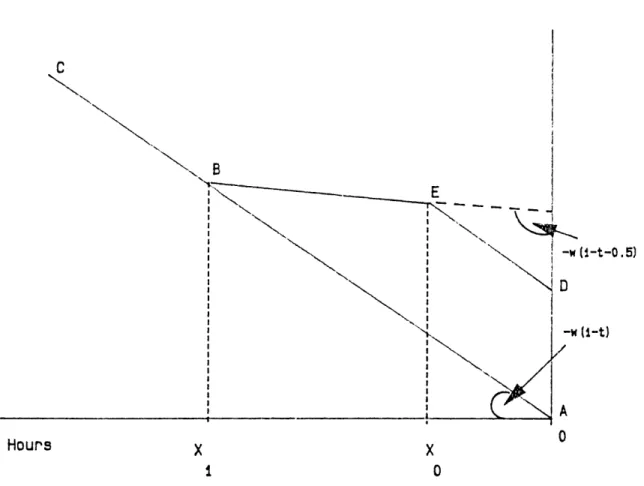
exhausted.5 The tax schedule yields the familiar non-linear budget constraint depicted in figure 1. Prior to age 62, an individual faces the budget set ABC which is governed by the after tax wage w(1-t). At age 62, the individual is eligible to receive a basic benefit level of B if he retires. Up to an earnings level of X., the marginal incentives are unchanged so that the slope of the budget line is given by the negative of the earlier after-tax wage. At that point, the earnings test taxes the basic benefit at a 1:2 rate so that the slope of the budget line is now w(1-t-0.5). At X₁, the basic benefits are exhausted and the individual's budget set lies along the BC portion of the original segment. The total budget set under the Social Security system is thus DEBC.

Several analysts have seized upon the implications of figure 1 as a reason for concern with the work-incentive effects of the Social Security system. The unambiguous conclusion that Social Security reduces labor force participation does not, however, follow

immediately. Drawing inferences based upon figure 1 alone can be misleading since the diagram does not fully capture the relevant incentives. In particular it ignores the life-cycle nature of the choices involved as well as salient features of the Social Security

5

In 1981, the earnings test allowed a maximum of $6,600 in earnings before benefits were reduced.

Figure 1

-

Non-Linear Budget Constraint For Individual

Eligible for Social Security Benefits

Income

C

'K

E

KK~

IC

X

x

(1-t)

0

I0

Hours

system.

First, the existence of automatic benefit recomputation (ABR) implies that the return to work consists of increments to Social Security wealth in addition to earnings. The effects of ABR have been outlined in some depth by Blinder, Gordon and Wise (BGW) [1980]. In brief, the Social Security benefits that are received by an

individual upon retirement are calculated on the basis of the

lifetime work history. The first step involves calculating a measure of the individual's average monthly wages (ANW) which, to simplify somewhat, are computed by averaging over the T highest years of earnings in covered employment.6 The primary insurance amount (PIA) is obtained by applying the AMW to a progressive benefit formula. An unmarried individual retiring at the base age of 65 receives the PIA; a married couple receives either the sum of the individual

entitlements, or 1.5 times the single benefit level, whichever is greater. An individual who works for an additional year is able to

6_{The value of T depends upon the age of the individual and the year}

in which the computation takes place. For the individuals in the RHS, the relevant formula is

T = min(year,yr65) - 1956

where year = the year of the computation and yr65 = the year the individual turns 65. For currently retiring individuals, the number of years of computation is the minimum of the current age less 26,

and 36.

7

Beginning in 1974, benefits were indexed for inflation. The PIA is multiplied by the ratio of the growth in the CPI over the interval

from 1974 to the year benefits are received. As Diamond (1977] notes, this creates significant overindexation for inflation since

substitute current earnings for the minimum of the earnings currently used in the computation of the AMW. Individuals with upward sloping age-earnings profiles are likely to have much higher current earnings than those received in the lowest earnings period, especially in an

inflationary environment, so that the increases in the AMW and hence in future Social Security benefits can be significant. BGW perform calculations which suggest that under pre-1977 law, the wealth effect is on the order of a 50% wage subsidy for a representative

individual.

Second, the effects of the imperfect actuarial adjustment mean that the relevant lifetime budget constraint can be improved by

additional work up through age 65. Actuarial adjustments are made to the basic benefit with the stated purpose of providing statistically fair increases and decreases in benefits for those accelerating or postponing retirement. Individuals who elect to retire prior to age 65 have their monthly benefits decreased to account for the longer expected period of time over which they will be receiving those benefits. The actuarial reduction is 5/9% for each month between ages 62 and 65 in which the individual does not draw benefits. No benefits are paid prior to age 62. Similarly, benefits are increased

the indexation is from a fixed date rather than from the date the individual turns 62, and since, prior to 1977, the AMW computations were based upon nominal income. From 1977 onward, the AMW is

computed using earnings indexed by the growth in overall earnings levels.

by 1/12% for each month without payment of benefits between ages 65 and 72.8 Calculations made by BGW indicate that these actuarial adjustments are fair or more than fair for the 62-65 period and less than fair for the post-65 period. Thus, there is an actuarial bonus to delaying retirement to age 65, but a penalty for delaying past 65.

The effects of ABR and actuarial adjustments are difficult to capture with a single-period model of this type, but if thought of as wage subsidies, can be represented by increases in the slope of the budget line under Social Security. For large enough wage subsidies, the income and substitution effects operate in opposite directions, with the substitution effect encouraging work. The result of the various income and substitution effects are such that the exact

relationship between Social Security and retirement is theoretically ambiguous. Furthermore, assessing the magnitude of the effects of Social Security upon retirement requires empirical analysis.

1.2 Partial Retirement

1.2.1 The Definition of Retirement

There is no natural way in which to define retirement,

consequently a variety of definitions for retirement have been used in the empirical literature. Among them are complete withdrawl from the labor force (Gordon and Blinder (1980]), transition from job held

8_{Recent legislation has allowed the full payment of benefits once an}

at the start of the sample (Fields and Mitchell [1984]),

self-reported status (Hausman and Wise [1985]), the receipt of pension income (Burkhauser (1979]), and work less than a specified number of hours (Boskin [1977]).

Difficulties arise with the use of each of these definitions. Under the definition based upon labor force participation,

individuals working a few hours a week but who are substantively retired and perhaps drawing pension benefits will be classified as working. Under a transition definition, individuals who make job changes totally unrelated to retirement will be classified as retired. Self-reported status suffers from being unrelated to

observable economic activity. Available evidence suggests that using pension receipt as an indicator of retirement may be misleading

because many individuals who are not working at all receive no pension income (Diamond and Hausman [1984]). Finally, there is a certain arbitrariness to definitions based upon reduced work effort. What is most disturbing is the result that these definitions often yield conflicting classifications.9

Underlying these definitional difficulties is the fact that a single form of retirement is unable to capture the behavior of

individuals who are not employed in a "standard" full-time job, but

9_{To see the problems involved, consider the case of an individual who} reduces the number of hours worked per week in the same job by a third in order to collect a newly vested partial pension.

are still in the labor force. It is this fundamental problem that motivates the consideration of partial retirement in this paper.

Like full retirement, partial retirement can be defined in a number of ways, but central to the concept is a discontinuous, though not complete, reduction in work effort. An individual who wishes to reduce his work effort can do so by reducing the number of hours worked per week, by reducing the number of weeks worked per year, by

working less diligently during the time spent at work, or through some combination of the above. For the purposes of this study, partial retirement is defined as employment at a job in which the individual reports less than 35 hours of work per week or employment for less than 46 weeks (the weeks-equivalent of a 35 hour work

week).10 The definition corresponds to considering reductions in the hours and weeks worked, but ignores the unobservable measure of work effort.11

In the subsequent discussion, retirement of either form will be

10Weeks of unemployment are considered as weeks of employment when evaluating the latter measure. It is possible that individuals will report vacation time as weeks of no work so that the weeks definition will overstate the extent of partial retirement. This does not

appear to be a problem since almost all individuals who are

classified as partially retired under the weeks definition are also partially retired by an hours criterion.

11This definition suffers from the arbitrariness cited above. Among the studies that have considered partial retirement, Boskin [1977] and Zabalza et. al. [1980] use reduced hours of work; Gustman and

Steinmeier (1986] use self-reported status. The particular choice of definition used in this study is motivated in part by the questioning

patterns of the Longitudinal Retirement History Survey, and in part by a desire to base the definition on observed behavior.

referred to simply as retirement; where distinguishing between full and partial retirement is necessary, the appropriate qualifier will be used.

1.2.2 The Extent of Partial Retirement

Typically, analyses of retirement behavior have not considered the possibility of partial retirement and have defined a single form of retirement in one of the ways listed above. The notion that partial retirement is distinct from full retirement and should be treated separately in empirical work was first adopted by Boskin

[1977] and has been used by, among others, Boskin and Hurd [1978] and Zabalza et. al. (1980]. For the most part, however, researchers have utilized the concept of a single form of retirement.12

Recent work by Gustman and Steinmeier [1984] has shed some light on the extent of partial retirement. Using a sample drawn from the Longitudinal Retirement History Survey (RHS), they find that of those individuals who are observed to transit from full-time employment, approximately 28.2% partially retire. Over one-third of the

individuals studied report partial retirement in at least one of the four sample periods. These results are corroborated by Zabalza et. al. who report that their sample of elderly in Great Britain exhibits a well-defined bimodal distribution of hours worked, and by Parnes

1 2_{Relatively comprehensive surveys of the literature are provided by}

and Nestel [1981] who find that about 20% of their 1966-1975 National Longitudinal Survey sample reports post-retirement labor market

activity.13 Noreover, given current and anticipated future reductions in mortality rates and the resulting increases in longevity, the importance of partial retirees in the economy is

likely to grow over time.

Drawing upon data derived from the RHS, I find results that are similar to those of Gustman and Steinmeier, despite the use of an hours/weeks worked definition rather than self-reported status. Table 3 shows the number of individuals retiring at various ages,

aggregated across cohorts, broken down by type of retirement. The censoring category refers to those individuals who do not retire over the sample interval. The age at censoring is therefore the last age at which they were observed. The sample includes only those

individuals who retire after age 57. Since less than 1/2 of one percent of the individuals report retirement prior to age 58, and of those individuals, one-quarter appear to be subject to coding error, or are highly unrepresentative of the population as a whole, this

13In the latter study, retirement is defined by self-reported status. Among those classified as retired who reported having worked in the 12 month period prior to the 1976 survey, approximately 17 percent reported working more than 2,000 hours. Assuming work over the entire year, this translates into about 38.5 hours per week. 23 percent of the sample reported working more than 29 hours per week, 42 percent more than 19 hours per weekk,and 71 more than 10 hours per week.

Table 3 - Age distribution of retirement or censoring by type of first retirement, 1633 person RHS subsample.

Type of Initial Retirement Age at Retirement (Number of Persons)

Full Partial Censored Total 58 59 60 61 62 63 64 65 66 67 68 69 70 71 72 73 Totals 4 6 13 27 86 124 117 275 173 67 36 19 14 5 7 2 975 1 0 11 14 61 56 130 75 65 52 20 16 5 6 1 2 515 0 0 7 6 7 7 4 8 1 1 29 23 16 14 12 8 143 5 6 24 41 147 180 247 350 238 119 56 35 19 11 8 4 1633

Note: Based upon author's calculations. The various forms of retirement are defined in the text.

procedure should not create undue biases. 1 Focusing first on the number of individuals in each retirement class, table 3 shows that out of a sample of 1633 individuals, over 500 partially retire. Since 975 individuals move directly to full retirement, a little under a third of those who actually retire over the sample period partially retire. While a bit higher than the figure found by

Gustman and Steinmeier, the observed fraction is certainly comparable in magnitude.

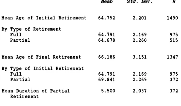
In table 4 I present data on mean age of retirement for various types of retirement. To see the impact of differing definitions, note that if one defines retirement to be the first instance of full or partial retirement, the mean retirement age is 64.75; this average age is in contrast to a mean retirement age of 66.19 resulting from a definition based upon complete withdrawl from the labor force.

Breaking down the mean age of initial retirement, the mean age for partial retirees is 64.68, slightly less than the corresponding age of 64.79 for full retirees.

The closeness of these mean values hides a considerable amount of work activity. For those individuals who partially retire and are

14The ages of retirement for these individuals include 36, 46 and 48. The calculations of the percentage who are excluded on the basis of retirement age are based upon preliminary work utilizing a slightly different subsample than the one used in the estimation. While it can be argued that this exclusion creates a form of self-selection which biases the results, it seems more likely that these individuals differ from the rest of the population in the way that retirement decisions are made and should therefore be considered separately.

Table 4 - Mean age of retirement RHS subsample.

under different retirement paths,

mean

Mean Age of Initial Retirement By Type of Retirement

Full Partial

Mean Age of Final Retirement By Type of Initial Retirement

Full Partial

Mean Duration of Partial Retirement 64.752 64.791 64.678 66.186 64.791 69.841 5.500 Std. Dev. 2.201 2.169 2.260 3.151 2.169 2.269 2.037 N 1490 975 515 1347 975 372 372

Note: Based upon author's calculations. All samples are limited to completed spells for the retirement in question. The partial

retirement category for mean age of final retirement refers to those individuals observed to fully retire who first partially retired.

subsequently observed to fully retire, the mean duration of partial retirement is approximately 5.5 years. As one might expect, the duration is negatively correlated (-0.446) with the age of initial retirement so that individuals who retire earlier remain in partial retirement for a longer period of time. The mean duration is in excess of the durations studied by Gustman and Steinmeier who find that most of those who partially retire spend a relatively short period of time, one to two years, in that state. The discrepancy results, no doubt, not only from the differences in the definitions of partial retirement, but also from the differing definitions of full retirement since I use a definition based upon complete withdrawl from the labor force while Gustman and Steinmeier use self-reported full retirement. The latter definition will classify as fully retired individuals listed as partially retired by my definition.

In addition to differences between mean retirement ages, there are differences in the distribution of retirement ages. Table 3 shows that the number of individuals classified as retiring at a given age rises slowly up to age 62, then sharply through age 65, declining in subsequent years. The same is true when considering either full or partial retirees alone, though the number of partial retirees is generally smaller than the corresponding number of full retirees. The modal age for those who partially retire is age 64, earlier than for those who first fully retire, a result that is

reflected in the slightly lover mean age of retirement. Somewhat surprisingly, the total number of partial retirees at age 64 is greater than the corresponding number of full retirees. The relationship is reversed at virtually every other age.

More informative, perhaps, are simple calculations of the hazard rates for both types of retirement. These represent the probability of retiring at a given age conditional on not having retired prior to that age. Thus, the full retirement hazard for a 63 year old

individual is the probability that he fully retires at age 63, given that he has not retired previously. The hazards are calculated by dividing the number of retirees of a given type, (full or partial) at a given age, by the number of unretired individuals up to that age.15

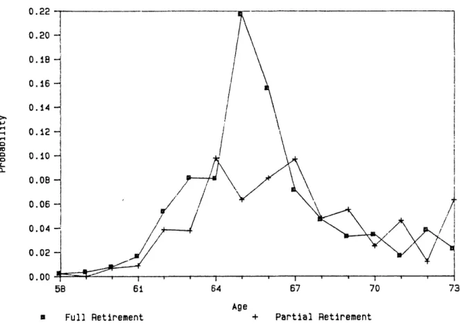
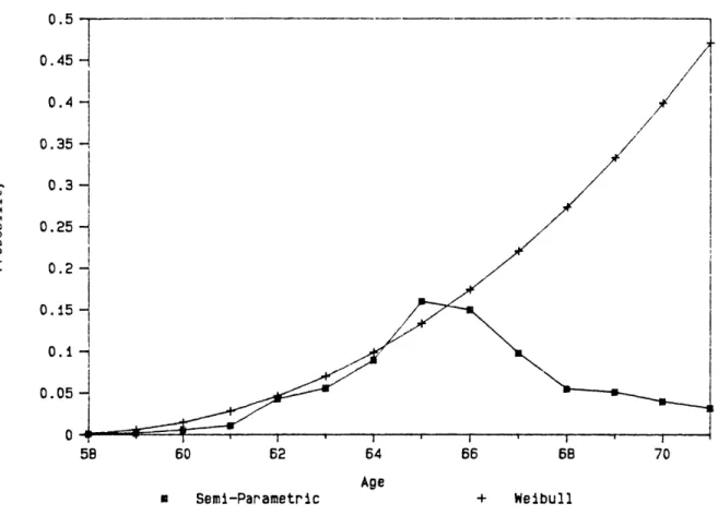
Hazard rates for both forms of retirement are depicted in figure 2. Up to age 64, the hazards are similar in shape, with the full retirement hazard rising somewhat faster than the partial retirement hazard. There is a pronounced spike in the full retirement hazard at age 65 that is not present for partial retirement. If anything, the partial retirement hazard is bimodal, with a pronounced drop in the hazard at age 65 and peaks at age 64 and 66. Moreover, with the exception of ages 65-66, the partial retirement hazard lies above the full retirement hazard for most ages greater than 64. The difference

1 5_{It is easy to show that this is the maximum likelihood estimator of} the hazard rate for a homogeneous sample. This estimator is referred to in the statistics literature as the Kaplan-Meier estimator.

Figure 2

-

Sample Hazard Rates for Retirement

Full and Partial Retirement

0.224 0.20 0.18 0.16 0.14 0. 12 0* 0.10 0.08 0.06 -0.02 58 61 64 67 70 73 Age + Partial Retirement 0 Full Retirement

in hazards suggests that individuals who fully retire are retiring at the "standard" ages close to 65 and that, conditional upon not

retiring at those ages, an individual is more likely to move into partial retirement prior to full retirement than directly to full retirement.

The most important conclusion that I draw from the comparison of sample hazard rates is that the age-profiles suggest that different factors are leading to the decisions to retire fully or partially. Estimation of a model which does not distinguish between the two will confound the differences in behavior implied by the different

hazards. Two cautions should be expressed at this point. First, underlying the results depicted in figure 2 is the assumption that the population is homogeneous. This assumption is obviously

untenable and the econometric specifications developed in the paper are designed to relax this restriction. Second, the sample sizes become relatively small as one moves out to the right tail of the age distribution so that some caution should be taken in drawing

conclusions based upon the shape of the hazards at these later ages. Still, the hazards differ by enough so that it should be safe to conclude that distinguishing between full and partial retirement is important.

2. The Existing Literature

Boskin [1977] who analyzed the labor force participation of a 131 observation sample of households, finding very large negative effects for Social Security. Based upon estimates from a first-order Markov model of transition probabilities, he concluded that the existence of the Social Security system has increased the annual probability of retirement by 40 percent. The 40 percent figure suggests that Social Security is responsible for the bulk of the observed decline in labor force participation in the past few decades.

This view was challenged by Gordon and Blinder [1980] who, building upon their work with Wise [1980] on the institutional characteristics of Social Security, postulate a three-period life-cycle model of labor-leisure choice in which individuals presently choose to work or to retire as the market wage is greater than or less than a reservation wage. Based upon estimates from this model GS find that Social Security has rather small effects on retirement behavior--a change in the Social Security wealth to income ratio of 0.01 (about 14 percent) has a negligable impact upon retirement probabilities. 16

Later work by, among others, Fields and Mitchell [1984], Boskin and Hurd (1984], Burkhauser (1979], Zabalza et. al. (1981] and

1 6_{The Gordon and Blinder finding that Social Security has almost no} effect upon retirement stands virtually alone in the empirical literature, and is difficult to reconcile with the large spikes in retirement hazards coincident with Social Security eligibility found by Hausman and Wise [1985] and others.

Burtless [1986], using a variety of techniques come to a number of often conflicting conclusions. This smorgasbord of results led Aaron

to conclude in 1984 that "...about all that can be said is that a preponderance of studies, whose evidentiary value is quite low, concludes that Social Security has an indeterminate impact upon retirement behavior."

Among the many studies which consider the determinants of

retirement behavior, perhaps the closest to the present analysis are the recent study of partial retirement conducted by Gustman and Steinmeier [1986] and the risk models of retirement developed by Hausman and Wise (1985] and Diamond and Hausman [1984]. In this paper, I combine the concern with partial retirement of Gustman and Steinmeier with the statistical techniques developed in the Hausman and Wise and Diamond and Hausman papers, while relaxing some of the less satisfactory assumptions in both.

Gustman and Steinmeier (GS) estimate a structural model of

retirement in which partial retirement is represented by the presence of an alternative wage-leisure offer. Demographic and other control variables enter into the specification solely through the preference for leisure, while economic variables enter through the lifetime budget constraint. They find moderate effects of economic variables upon retirement, with a hypothetical 50 percent increase in

compensation streams for full and partial retirement, pensions, and Social Security reducing the percentage of individuals working

full-time by about 10 percentage points for individuals up through age 64, and by a smaller amount for older individuals. This increase in the number of retirees is distributed unevenly across the two types of retirement.

While the GS paper is a careful analysis of the partial retirement issue and as such is an important contribution to the analysis of retirement behavior, the overly simple structure of their model makes it difficult to disentangle the effects of Social

Security from the effects of, say earnings. 7 In fact, it is a requirement of the GS model that the effects of a dollar increase in

the present discounted value (PDV) of Social Security benefits

exactly equal a corresponding increase the PDV of earnings or wealth. If it is believed that individuals discount future Social Security benefits at a different rate than other income streams, this

assumption is untenable. The assumption of identical discount rates is likely to be a problem given evidence of liquidity constraints, since individuals are prohibited by law from borrowing against Social Security wealth.18 Furthermore, the GS assumption that individuals face a single alternative wage-leisure offer for partial retirement

17In all fairness, this is the result of the extreme complexity of their estimation technique.

18See Paquette [1985] for evidence that elderly individuals face constraints on their liquidity. Diamond and Hausman [1984] also provide evidence from the National Longitudinal Survey of Older Males that supports this result.

is open to criticism.

The HW and DH studies both take a different approach to analyzing the determinants of retirement. Building upon the

statistical literature and the work of Lancaster [1979] they specify functional forms for the conditional probability of retirement and use these to estimate probabilities of retirement at different ages. Using a sample drawn from the RHS, HW estimate a hazard model of

retirement which indicates that Social Security and other economic variables have significant effects upon retirement. According to their calculations, the increase in Social Security benefits over the past two decades may account for up to one-third of the decrease in labor force participation. DH estimate a hazard model of retirement for a slightly younger sample of National Longitudinal Survey of Older Men (NLS) individuals. Their results are similar in character to the HW results.

Unfortunately, these latter two studies assume a single form of retirement. Moreover, in the specification of the hazard functions, strong parametric restrictions are placed upon the behavior of

individuals. These restrictions take the form of simple functional form specifications for the effects of aging upon retirement

probabilities.19 In this paper I relax both the assumption of a

19The same is true for the dual-risk model estimated by DH for

re-employment and retirement of the unemployed. The DH restrictions involve linearity of the latent random variables for time to

re-employment and time to retirement with respect to the covariates. This specification implicitly places strong, non-testable functional

single form of retirement and the parametric restrictions upon behavior.

3. Econometric Specification

The econometric techniques employed in this paper are derived from the extensive literature on hazard models.20 Hazard models have enjoyed considerable popularity in empirical work since Lancaster

[1979] introduced them to the economics profession in his study of unemployment durations. The previously mentioned studies by HW and DH apply these techniques to the study of retirement behavior. This paper, in contrast to earlier studies, uses techniques developed recently by Han and Hausman [1986) to estimate semi-parametric dual risk models that allow for correlation between the risks. In the retirement context, the two risks of interest are the probabilities of full and partial retirement. The technique is outlined in some detail in the remainder of the section.

It should first be noted, however, that despite an obvious

relationship to other discrete choice models such as the logit, these techniques employ reduced forms which are not grounded in maximizing theory. While one can think of an individual solving a complicated

form restrictions upon the shapes of the baseline hazards.

2 0_{These models are also referred to as failure time models. Standard}

references in the statistical literature are Cox and Oakes [1984] and Kalbfleisch and Prentice (1980].

dynamic stochastic programming problem to determine an optimal retirement date, such a model cannot be linked directly to these hazard estimates. Intuitively, however, the model that underlies

these specifications is one in which individuals solve a maximizing problem by making sequential labor-force participation decisions,

comparing the utility received from retiring at a given time with the utility from continuing to work as well as the utility received from accepting an alternative, partial retirement wage-leisure offer and retiring at a later date.21 The utility comparisons are influenced both by the age at which the decisions are being made and by the effects of other, individual specific factors.

3.1 Single Risk Estimation

Generally, an observation on a failure time can be of two types. First, the time of failure can be the direct result of the hazard process under investigation. Thus, a direct failure time observation on retirement would provide the age at which an individual is

observed to retire. Alternatively, the time of failure can result from right censoring of the data. Right censoring occurs when the period over which the individual is surveyed is not long enough for

2 1_{These offers might be thought of as coming from a distribution of}

offers in much the same way that job offers are received by an

unemployed individual (see Katz [1985]). Much more thought needs to be applied to the question of the best way in which to combine the retirement and reservation wage frameworks.

observation of a direct failure time. For example, the ending of the RHS sample period in 1979 censors failure times for those individuals who are still working at that date.

A failure time observation can therefore be characterized by the time of failure and by the type of failure, actual or censored.

Suppose that failure time data of the form (t.,5.,X ), i=1,...,N, are observed where

t. is the observed failure time for individual I

a is a censoring indicator where a= 0 ohercnsored failure X is a k-vector of covariates.

In the retirement context, t represents the age of retirement if 8=0, or the age that the individual leaves the survey if 8=1. It should be pointed out that in most of the discussion that follows, t. is an assumed to be a discrete approximation to the true failure time. The use of a discrete approximation results from the fact that in most data available to economists, observations on individuals are made at discrete points in time. For the RHS survey, the discreteness of the data results from the fact that observations on individual employment status may only be made at year intervals. Thus, an observed failure time of t. implies that the true failure time lies in the interval

(t -1,t ].

true failure time. Suppressing the individual subscript, I assume that the conditional probability of retirement at time t can be written in the following form

(3.1.1) h(t) = lim+ Pr(t < T ( t + 4 I T > t)

4-.

= A(t) exp(Xp).

where A(t) is a non-negative function of age which represents the effect of time upon the conditional probability. This model is the proportional hazards specification of Cox [1972). It derives its name from the fact the effects of the covariates X operate

proportionally upon the baseline hazard A(t) through the parameters

A-Two functions of h(t) are of additional interest. First, the survivor function, Q(t), gives the probability that the individual failure time is greater than t so that the individual is observed not to have failed at time t. In the present analysis, survival

corresponds to noting that an individual has not yet retired at a given age. Second, the unconditional density function for failure time, f(t), is a standard probability density function for the random variable for failure time, T. Both can readily be written in terms of h(t):

(3.1.2) Q(t) = Pr(T > t) = exp(- f h(s) ds),

(3.1.3) f(t) = lim+ Pr(t < T < t + J) = h(t) Q(t).

The complete specification of the likelihood of an observation for either continuous or discrete data is possible using a combination of

(3.1.2) and (3.1.3).

Unobservable individual effects are readily incorporated into the specification. Suppose that there is an additional random component to the hazard function, 0, which enters multiplicatively. Then (3.1.1) becomes

(3.1.4) h(tje) = e A(t) exp(Xp) = 9 h(t).

where

e

(3.1.5) Q (t) E E9 Q(t je)

= E9 exp(- f h(s|e) ds)

S

where o2 is the variance of the gamma distribution.

It is a straightforward exercise to write out, for the entire sample, the log-likelihood functions associated with each of these specifications. For illustrative purposes, I consider two cases. First, if there is continuous data and no heterogeneity, the

log-likelihood function is given by

N

(3.1.6) log L(p) =

1

i=1

while if heterogeneity is present and there is discrete data of the form described above, the log-likelihood is

N

(3.1.7) log L(p,o) = Z (1-6 ) log (Q (t -1) - Q (t ))

i=1

*

+ _{6. log Q (t )}

Most commonly, the specification has been completed by choosing a functional parameterization of the baseline hazard A(t)--often a single-parameter Weibull (A(t) = a t "~). Unfortunately, it has been established that results obtained from maximum likelihood estimation of these functions are sensitive to the choice of a distribution for the heterogeneity parameter and the choice of functional form for the

baseline hazard.22 To reduce the biases resulting from functional form restrictions, I adopt the semi-parametric HH approach of

estimating (3.1.6) and (3.1.7) parametrically with respect to the p, but with no restrictions on the form of A(t).

To see how the technique works, note that (3.1.3) can be rewritten as the transformed model

(3.1.8)

It

X +

t

(3.1.9) 1t log ft A(s) ds

where e has an extreme value distribution. Rewriting the likelihood in the regression form involves a simple transformation of variables, a process which is outlined in greater detail in Appendix 1.

Suppose now that an individual is observed to have retired at time t where t is again a discrete approximation to the actual

failure time T. The probability of observing a failure at time t for a given individual is given by

(3.1.10) Pr(t-1 < T t) =

+x

fit-1+XA

The estimation technique involves treating the 1 t-functions of the

baseline hazard as a parameter for each of the T potential failure periods and estimating them jointly with the

p.

otherwise, the log-likelihood for the entire sample corresponding to (3.1.6) can be written as

(3.1.11) log L(P,1) N T

= Z yi (6i log

fe)

i=1 t=1 rt+xp

+ (1-68) log t +XP (e) de

where (1 = 1 1 ,**. 1). Since s has an extreme value distribution, the specification corresponds to an ordered logit likelihood, with

the categories determined by the T failure times.23 The addition of heterogeneity to the model is straightforward, and is presented in Appendix 2.

3.2 Competing Risks Estimation

The extension of the semi-parametric technique to the competing

2 3

As might be expected, assuming that the e has a standard normal distribution yields essentially the same parameter estimates (after scaling for the unequal variances) except in the extreme tails of the distributions. Both models are easy to compute since algorithms for computing the CDFs are well-known. This finding is analagous to the results for the logit and probit models.