Computation of Nonlinear Hydrodynamic Loads on
Floating Wind Turbines Using Fluid-Impulse Theory
The MIT Faculty has made this article openly available.
Please share
how this access benefits you. Your story matters.
Citation
Chan, Godine Kok Yan et al. “Computation of Nonlinear
Hydrodynamic Loads on Floating Wind Turbines Using
Fluid-Impulse Theory.” ASME 2015 34th International Conference on
Ocean, Offshore and Arctic Engineering, 31 May- 5 June, 2015, St.
John’s, Newfoundland, Canada, ASME, 2015. © 2015 by ASME
As Published
http://dx.doi.org/10.1115/OMAE2015-41053
Publisher
American Society of Mechanical Engineers (ASME)
Version
Final published version
Citable link
http://hdl.handle.net/1721.1/109579
Terms of Use
Article is made available in accordance with the publisher's
policy and may be subject to US copyright law. Please refer to the
publisher's site for terms of use.
†Email address for correspondence: [email protected]
COMPUTATION OF NONLINEAR HYDRODYNAMIC LOADS ON FLOATING WIND
TURBINES USING FLUID-IMPULSE THEORY
Godine Kok Yan Chan†
Massachusetts Institute of Technology (MIT) Cambridge, Massachusetts 02139, USA
Paul D. Sclavounos MIT
Cambridge, Massachusetts 02139, USA Jason Jonkman
National Renewable Energy Laboratory (NREL) Golden, Colorado 80401, USA
Gregory Hayman NREL
Golden, Colorado 80401, USA
ABSTRACT
A hydrodynamics computer module was developed to evaluate the linear and nonlinear loads on floating wind turbines using a new fluid-impulse formulation for coupling with the FAST program. The new formulation allows linear and nonlinear loads on floating bodies to be computed in the time domain. It also avoids the computationally intensive evaluation of temporal and spatial gradients of the velocity potential in the Bernoulli equation and the discretization of the nonlinear free surface. The new hydrodynamics module computes linear and nonlinear loads—including hydrostatic, Froude-Krylov, radiation and diffraction, as well as nonlinear effects known to cause ringing, springing, and slow-drift loads—directly in the time domain.
The time-domain Green function is used to solve the linear and nonlinear free-surface problems and efficient methods are derived for its computation. The body instantaneous wetted surface is approximated by a panel mesh and the discretization of the free surface is circumvented by using the Green function. The evaluation of the nonlinear loads is based on explicit expressions derived by the fluid-impulse theory, which can be computed efficiently.
Computations are presented of the linear and nonlinear loads on the MIT/NREL tension-leg platform. Comparisons were carried out with frequency-domain linear and second-order methods. Emphasis was placed on modeling accuracy of the magnitude of nonlinear low- and high-frequency wave loads in a sea state. Although fluid-impulse theory is applied to floating wind turbines in this paper, the theory is applicable to other offshore platforms as well.
KEYWORDS
Wave-structure interactions, Fluid Impulse Theory
INTRODUCTION
The offshore wind industry has the potential to grow rapidly for a number of reasons. Wind is an inexhaustible and clean energy source. The horizontal-axis wind turbine is a mature technology. Vast wind resources exist in the offshore environment with stronger and steadier wind speeds allowing for significantly higher capacity factors than those encountered over land. The logistics of the offshore environment favor large multimegawatt turbines in the 6- to 10-MW range. These turbines can be easily assembled, transported to, and installed at the offshore wind power plant site. The support structure of offshore wind turbines can be either a bottom-mounted structure in shallow waters or a floating platform if the water is deeper than about 50 m. The wave loads exerted on these foundations by ambient sea states over the life of an offshore wind power plant must be properly modeled and predicted so that safe and cost-effective support structure designs can be developed.
The evaluation of the wave loads on offshore platforms is typically carried out either by Morison’s equation or by frequency-domain panel methods with appropriate time-domain transforms for transient analysis. Morison’s equation is a strip-theory-based time-domain method for slender structures. The method accounts for fluid inertia, added mass, and viscous effects by selecting appropriate added mass and drag coefficients. Morison’s equation also permits the treatment of strong nonlinearities in the vicinity of the waterline arising from steep ambient waves. Frequency-domain methods, on the other hand, are applicable to large-volume platforms and model linear and nonlinear potential-flow effects by solving first- and second-order free-surface problems. This leads to the computation of linear and quadratic transfer functions (QTFs). The time-domain fluid-impulse method presented in this paper
Proceedings of the ASME 2015 34th International Conference on Ocean, Offshore and Arctic Engineering OMAE2015 May 31-June 5, 2015, St. John's, Newfoundland, Canada
OMAE2015-41053
bridges the gap between Morison’s equation and frequency-domain methods. It can be used for both slender and large-volume offshore structures and allows for the modeling of higher-order transient nonlinear effects in the vicinity of the waterline.
In this study, the fluid-impulse method is applied to the computation of the nonlinear surge diffraction force on the Massachusetts Institute of Technology (MIT)/National Renewable Energy Laboratory (NREL) tension-leg platform (TLP), which supports a 5-MW wind turbine. Previous studies have carried out simulations for floating wind turbines using Morison’s equation and frequency-domain methods. Investigators carried out computations of the loads and responses of TLP floating wind turbines and documented them in [1-3]. Simulations for the Hywind Spar floating wind turbine structure based on Morison’s equation were reported by [4]. For the International Energy Agency Offshore Code Comparison Collaboration (IEA OC3) Spar, simulations were reported by [5]. For the semisubmersible WindFloat structure, simulations were presented by [6]. In [7], simulations for the IEA OC3 Continued (OC4) semisubmersible were documented.
The conclusions from the simulations reported in these and other studies are summarized here. There is good agreement between methods predicting the linear potential-flow loads from Morison’s equation or frequency-domain methods. The accuracy of Morison’s method deteriorates as the wavelength of the ambient wave decreases and becomes comparable to the diameter of a cylindrical floater. The agreement between various methods is less satisfactory for predicting the nonlinear low- and high-frequency loads and responses partly because the underlying modeling assumptions differ and partly because the accurate computation of the sum- and difference-frequency QTFs is a complex and time-consuming task. Because it is a time-domain method that may treat slender and large-volume structures, the fluid-impulse method developed by [8,9] addresses the gap between the long-wavelength approximations in the time-domain Morison-based method for slender members and frequency-domain approaches. In addition, the fluid-impulse method allows the evaluation of second-order and higher-order nonlinear effects via compact force expressions that circumvent the discretization of the free surface by taking advantage of the analytical structure of the time-domain Green function.
Viscous effects are not addressed in this paper, but they may contribute a significant component to the sea-state loads on bottom-mounted and floating wind turbine substructures. They can be accounted for by including Morison-type viscous force terms in the fluid-impulse theory. The advent of powerful multicore computational clusters, the growing maturity of computational fluid dynamics, and the availability of promising high-Reynolds-number turbulence models for massively separated flows [10]; however, offer a promising avenue for the future treatment of viscous effects by overlaying the fluid-impulse theory and the Navier-Stokes equations.
FLUID-IMPULSE THEORY FORMULATION
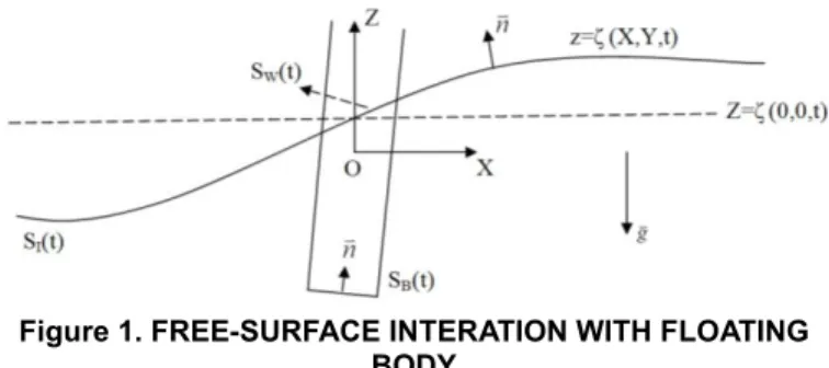
Figure 1 illustrates a platform floating on a free surface interacting with a nonlinear ambient wave assumed to be irregular. The reference coordinate system (X,Y,Z) is fixed in space with its origin located on the calm water surface with the positive Z-axis pointing upward. The free-surface elevation
resulting from the ambient wave is denoted by the solid line. The dashed line defines a horizontal plane intersecting the Z-axis at the local elevation of the ambient wave profile. The acceleration of gravity is g and the water density is ρ.
Figure 1. FREE-SURFACE INTERATION WITH FLOATING BODY
In Figure 1, the ambient wave velocity potential is denoted by
I( , , , )X Y Z t and the disturbance radiation/diffraction potentials are denoted by
( , , , )X Y Z t . Both are subject to the Laplace equation in the fluid domain as2 2 2 2 2 2 0. X Y Z (1)
On the instantaneous position of the body boundary ( )
B
S t
, the normal velocity of the radiation potential is equal to the normal velocity of the body boundary Unbecause of its oscillatory motions , ( ). n B U on S t n
(2)In the diffraction problem, the diffraction potential offsets the ambient wave normal velocity on SB( )t
, ( ) I B on S t n n
(3)For notational simplicity, the radiation and diffraction (RD) potentials are hereafter denoted by the same symbol, with the body boundary conditions from Eqs. (2) and (3) applying for each potential, respectively.
The Fluid Impulse Theory (FIT) derived by [8] linearizes the disturbance RD potential
about the ambient wave surface S tI( ) exterior to the body waterline as2 2 g Z 0, on S tI( ). t (4)
The conventional definition of the force and moment acting on the body follows from the integration of the hydrodynamic pressure obtained from Bernoulli’s equation over the instantaneous body wetted surface
( ) ( ) ( ) 1 ( ) ( ) ( ) 2 ( ) 1 ( ) ( ) ( ) 2 . I I I SB t I I I SB t F t gZ nds t M t gZ t X n ds
(5)The evaluation of the nonlinear hydrodynamic force and moment given by Eq. (5) requires the computation of the partial time and space derivatives of the disturbance potential over the instantaneous wetted surface of the body. This computational task requires fine panel meshes that lead to slow convergence in the evaluation of nonlinear forces.
The FIT formulation circumvents the computation of gradients of the disturbance potential by deriving new expressions for the hydrostatic and hydrodynamic forces summarized in the following sections. The total force in Eq. (5) is decomposed into a number of components
( ) H( ) F K( ) B FS.
F t F t F t F F (6) Only these forces are discussed in the remainder of this section. The definition of the moments can be found in the original FIT article [8].
Nonlinear Buoyancy Force
The hydrostatic force acting on the body takes the following form
( ) ( ) .
H W
F t
g t k (7)In Eq. (7), k is the unit vector pointing in the positive Z-direction and W( )t is the volume enclosed by the body wetted surface
( )
B
S t
and the nonlinear ambient wave surface interior to the bodySW( )t , defined in Fig. 1. The nonlinear hydrostatic force given by Eq. (7), then, always points upward. In the classical definition of the nonlinear body force obtained by integrating the hydrodynamic pressure from Bernoulli’s equation in Eq. (5), the nonlinear hydrostatic force depends on the shape of the body wetted surface and does not necessarily point upward. Equation (7) extends the classical Archimedean buoyancy force in calm water to the unsteady case of nonlinear wave body interactions via the introduction of a time-dependent displacement bounded by the body wetted surface and a dynamic water plane area defined by the ambient wave. Froude-Krylov Impulse Force
This force takes the following form
( ) ( ) ( ) ( ) . F K I I SBt SW t W t d d F t n ds dv dt dt
(8) The surface integrations in Eq. (8) are carried out over the instantaneous intersection of the body boundary and the ambient wave profile, which is assumed to be known with the unit normal vector pointing inside the body. An additional integration is carried out over the ambient wave free surface interior to the body. An application of Gauss’s theorem provides an alternative definition of the Froude-Krylov impulse as the integral of the ambient wave velocity vector over the volume internal to the body wetted surface and its dynamic water plane area. The evaluation of the new Froude-Krylov force and moment requires knowledge of only the velocity potential of the ambient wave over the body boundary and not its partial time derivative or its spatial gradients.Radiation and Diffraction Body Impulse This force takes the following form
( ) . B SB t d F n ds dt
(9) The integration in Eq. (9) is carried out over the instantaneous body wetted surface defined by its intersection with the ambient wave profile. Again the evaluation of the forces and moments requires only the RD velocity potentials over the body boundary and not their partial time derivative or spatial gradients.Radiation and Diffraction Free-Surface Impulse Force This force takes the following form
( ) ( ) 2 2 ( ) 1 1 ( ) ( ) ... 2 FS SI t SI t I I SI t d F n ds k ds dt t d ds dt g t g t z
(10) The unit normal vector to the ambient wave free surface may be expressed in terms of the gradients of the free-surface elevation. Denoting by the order of magnitude of the ambient wave slope obtains the following, with errors quadratic in the wave slope
2 2 2 ( ( , , )) ( ( , , )) 1 1 ( ) . I I X IY I I X IY I X IY Z X Y t i j k n Z X Y t i j k O (11)Substituting Eq. (11) in Eq. (10), invoking the linearized free-surface condition, and considering the force in the X-direction obtains the following
2 ( ) ( ) 2 2 2 ( ) 1 ( ) ( ). 2 I I FS X SI t SI t I D SI t d d F ds ds g dt X t t X g dt t X d ds O dt t Z X g
(12) In summary, the nonlinear hydrodynamic force acting on a body floating in an ambient irregular wave of large amplitude has been derived as the sum of a nonlinear buoyancy force pointing upward and the time derivative of a sequence of impulses. The Froude-Krylov nonlinear impulse involves an integral of the ambient wave velocity potential over the instantaneous body wetted surface and the interior water plane area defined by the ambient wave elevation. The body RD nonlinear impulse involves an integral of the RD velocity potentials over the body wetted surface. The free-surface RD nonlinear impulse involves integrals of the RD disturbances over the infinite ambient wave free surface exterior to the body waterline.The forces discussed in this section are based on the assumption that the RD velocity potentials satisfy the linear free-surface condition over the ambient wave free-surface profile. Higher-order nonlinear effects can be accounted for by invoking the fully nonlinear free-surface condition and introducing quadratic and cubic nonlinearities as forcing terms in the right-hand side of the linear free-surface condition in Eq.
(4) via perturbation theory. Details on the treatment of these nonlinear effects are presented in [9].
INTEGRAL EQUATION FOR THE DISTURBANCE POTENTIAL
The disturbance potential
satisfies the linearized free-surface condition in Eq. (4) on the ambient wave free-surface S tI( ) illustrated in Fig. 1. The horizontal dashed planar surface illustrated in the figure intersects the Z-axis at the ordinate(0, 0, ) ( )
I t I t
. To take advantage of the analytical properties of the time-domain Green function, the free-surface condition (Eq. 4) is hereafter assumed to be valid on the planar surfaceZ
I( )t . This assumption is justified by the small slope of steep waves in a sea state. Introduce the new coordinate system centered on the dashed planar surface as follows ( ) I( ). x X y Y z t Z
t (13) The Laplace equation maintains its original form relative to the new coordinate system. The free-surface condition, satisfied by the disturbance potential relative to the new coordinates(x X y, Y z, Z I( ), )t t ( , , , )X Y Z t
, followsfrom these identities
2 2 2 2 2 2 2 2 ( ) 2 ( ) ( ) ( ) . I I I I z t t t z t t z t t t z t z t t z
(14)Introducing Eq. (14) in Eq. (4), the free-surface condition relative to the new coordinate system becomes
2 2 2 2 2 g I( )t z 2 I( )t z t I( )t 2 0,z 0. t z (15) For ambient waves of small steepness, terms involving the time derivatives of the incident wave elevation are of the order of KA relative to the leading order terms, where A is the characteristic amplitude of the ambient wave and K is the characteristic wave number. Consequently, the free-surface condition relative to the new coordinate system, with relative errors ofO( )
, becomes the following:2 2 g z 0, z 0. t (16)
The body boundary conditions in Eqs. (2) and (3) maintain their form because they involve only spatial derivatives. They are enforced on the instantaneous wetted surface of the body defined relative to the new coordinate system.
From the preceding analysis, it follows that the free-surface condition in Eq. (16) is enforced on the planar z=0 surface at each time step. Relative to this plane the body wetted surface is more submerged below z=0 when
I( )t 0 and less submerged when
I( )t 0. The vertical coordinate of a point of the body wetted surface is given byz Z
I( )t , where Z is the vertical coordinate relative to the earth-fixed frame.The boundary value problem for the disturbance potential becomes a body nonlinear time-domain free-surface problem subject to the linear free-surface condition. Invoking the time-domain Green function, a time-convolution integral equation can be derived for the disturbance potential along the lines of [11,12]. The disturbance velocity potential is represented by a distribution of sources over the instantaneous wetted surface of the body, as follows
( ) 0 ( ) 1 1 1 ( , ) ( , ) 4 ' ( , ) ( , , ). SB t t SB x t ds t r r d ds H x t
(17)The unknown source strength distribution ( , )t for t>0 is determined from the solution of the integral equation obtained by enforcing the body boundary condition as follows
( ) 0 ( ) 1 1 1 ( , ) ( , ) 4 ' ( , ) ( , , ) . SB t t SB n x t n ds t n r r d ds H x t
(18) The left-hand side of Eq. (18) is a known normal velocity on the body wetted surface for the RD problems via Eq. (2) and Eq. (3), respectively.Invoking the following notation,
2 2 2 1/2 2 2 2 1/2 ( , , ) ( , , ) [( ) ( ) ( ) ] ' [( ) ( ) ( ) ] , x x y z r x y z r x y z
(19)the time-domain Green function is defined as follows
(0) ( ) 0 0 1/2 2 2 1 1 1 ( , ) 4 ' 1 ( , , ) sin ( ) 2 ( ) ( ) . k z G x r r H x t dk gke gk t J kR R x y
(20)The integral equation in Eqs. (17) through (20) is solved by discretizing the instantaneous body wetted surface with planar panels and advancing the time-convolution integral ahead in time starting at t=0.
The panel mesh typically extends up to the deck above the free surface and its coordinates are defined relative to a body-fixed coordinate system. As a result, no re-meshing of the body wetted surface is necessary at each time step for large amplitude motions. A translation and rotation of the original panel mesh and the identification of the portion of the panel mesh that is wet at each time step are necessary. An essential attribute of the efficiency of the computational scheme is the fast computation of the memory component of the Green function defined by the second term in Eq. (20).
in a sea state and in Eq. (22). The solution of the integral equation in Eq. (18) provides the disturbance velocity potential
( , ),x t t 0
over the instantaneous position of the wetted surface via Eq. (17). The substitution of the incident and disturbance potentials in Eqs. (8) and (9) allows the evaluation of the fluid-impulse Froude-Krylov and body forces. This is carried out by first integrating the velocity potentials over the body wetted surface and then taking the time derivative of the resulting time-dependent integral. The evaluation of the partial time derivative and spatial gradients of the ambient and disturbance potentials is circumvented. The free-surface impulse force in Eqs. (10) through (12) is evaluated in the next section.FREE-SURFACE IMPULSE FORCE
The fluid-impulse force in Eq. (12) in the X-direction involves quadratic and cubic products of the incident and disturbance potentials. This force component, then, accounts for higher-order effects. Keeping the leading order quadratic effects in Eq. (12) for the free-surface fluid-impulse force in the X-direction obtains the following
2 0 0 . ID DD FS X FS X FS X ID I I FS X z DD FS X z F F F d F ds g dt x t t x d F ds g dt t x
(21)In Eq. (21), the free-surface impulse force is decomposed into two terms. The ID term involves cross-products of the incident and disturbance potentials, whereas the DD term involves a quadratic product of the disturbance potential. In addition, the integration is carried out over the shifted z=0 plane exterior to the instantaneous body waterline. The force defined by Eq. (21) is of second order in the incident and disturbance potentials with the latter satisfying the linear free-surface condition in Eq. (4). This force is of higher order if the disturbance potential satisfies the nonlinear inhomogeneous free-surface condition discussed in the next section.
The incident wave potential of an irregular wave train is represented by the linear superposition of plane-progressive waves with amplitudes obtained from the sea state spectrum and independent phases drawn from the uniform distribution. The velocity potential in deep water of a unidirectional irregular wave propagating at an angle relative to the positive X-axis is given by
cos sin 2 ( , , ) / . z i x i y i t i j j j j j j I j j j j igA x z t e g
(22)Second-order effects may be included in the definition of the ambient waves in deep or finite water depth by invoking the analytical solutions available in [13].
The evaluation of the infinite free-surface integral in the ID component of the free-surface impulse force can be carried out explicitly in terms of the source strength over the body wetted surface and the disturbance potential over the water plane area internal to the body surface. This was carried out by [9] and the result follows
2 cos sin ( ) cos sin cos ( , , ) ( , , ) ( , ) ( , , ) . ID I I X SW i t i i i SB z i x i y i t i I d F ds g dt x t t x A e K t K ds e igA x z t e
(23)The evaluation of the source Kochin function K and the integral over the internal water plane area involving the incident and disturbance potentials can be carried out easily using the solution of the integral equation in Eq. (18) for the source strength and the representation in Eq. (17) for the disturbance potential.
The infinite integral of the DD component of the free-surface impulse can also be reduced explicitly into a form that involves integrals of the memory component of the disturbance potential over the body wetted surface and the internal water plane area as described by [9]. The result follows
2 ( ) 1 1 1 1 1 ( ) 2 ( ) 2 ( ) ( ) 1 2 ( ) 1 2 2 1 2 0 ( ) ( , ) ( , ) 2 ( , ) ( , ) ( , , ). M DD X SB t M M M CW SW t M SB t F ds t dl n ds g t g t x t d ds H t
(24) The force components in Eqs. (8) and (9) involve the ambient and disturbance velocity potentials linearly, yet they account for nonlinear effects via the time dependence of the body wetted surface defined by its intersection with the ambient wave profile. The force components in Eqs. (23) and (24) involve quadratic products of the incident and disturbance potentials. In Eqs. (8), (9), (23), and (24), higher-order effects can be accounted for by including second-order effects in the definition of the ambient wave velocity potential. The computation of the forces in Eqs. (8), (9), (23), and (24) is described in the numerical results section.HYDRODYNAMIC PRESSURE
The local hydrodynamic pressure is of interest for structural analysis. The force expressions derived from the FIT theory rely only on the knowledge of the velocity potentials over the body boundary. The direct evaluation of the hydrodynamic pressure is circumvented, which leads to an efficient computational scheme with a coarse panel mesh. The evaluation of the local pressure is still possible, however. It involves a few simple steps as discussed in this section.
Using the methods described previously, the total velocity potential
I
is evaluated on the panels. Denote the velocity potential at the centroid of the ith panel at time t by( )t
and the velocity of that centroid as a point fixed on the body (and translating with its local velocity because of its rigid
body motions) by V ti( ). The convective time derivative of the total velocity potential along the path of the centroid of the ith panel over a time step t is defined by
( ) ( ) ( ) ( ). i i i i i i i D t t t Dt t D t V t Dt t (25)Solving for the partial time derivative of the total potential yields the following
( ) ( ) ( ) ( ). i i i i i t t t t V t t t (26)Therefore, the partial time derivative of the total potential at the centroid of the ith panel at time t can be evaluated in terms of the value of the velocity potential at the centroid of the same panel at time t t, the velocity of the panel centroid at time t, and the gradient of the total potential at the centroid of the ith panel at time t. The value and gradient of the incident wave component of the total potential are easy to evaluate analytically. The gradient of the disturbance potential is available from its definition in Eq. (17) as a distribution of sources over the body wetted surface.
The hydrodynamic pressure at the centroid of the ith panel follows from Bernoulli’s equation
( ) 1 ( ) ( ) 2 i i i i t p t t gZ t (27)
The velocity vector V ti( ) follows from the solution of the equations of motion of the platform.
ADDITIONAL NONLINEAR COMPONENTS
The second-order potential resulting from the nonlinear free-surface condition was not included in this study. The significance of the second-order potential will be evaluated and computed in future studies and the full nonlinear numerical results will be compared with experimental data.
NUMERICAL RESULTS
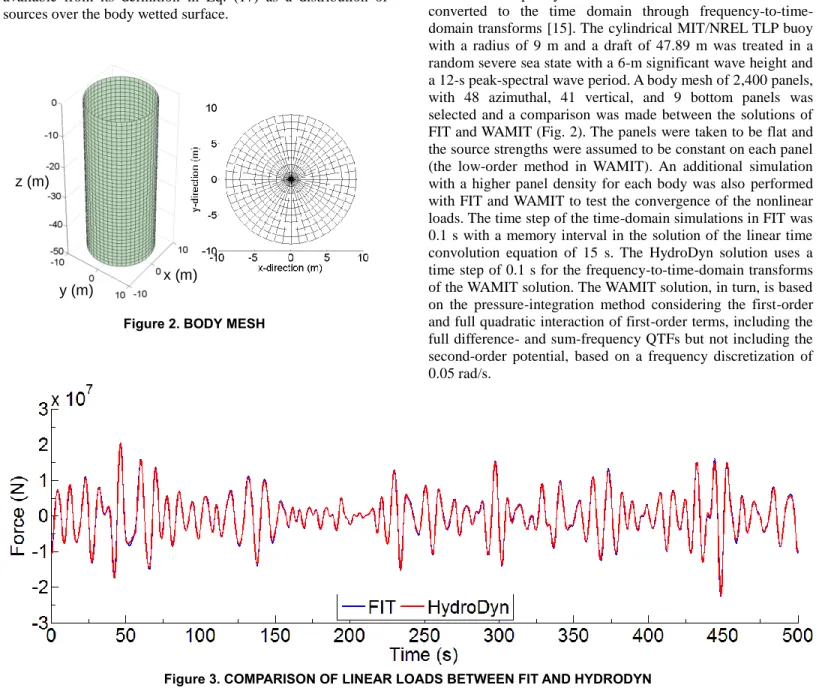
The fluid-impulse theory was implemented for the computation of the linear and nonlinear surge diffraction force on a truncated vertical cylinder in a new FAST module called FIT. The results were analyzed and compared with the potential-flow method of FAST’s HydroDyn module [14], based on frequency-domain solutions from WAMIT and converted to the time domain through frequency-to-time-domain transforms [15]. The cylindrical MIT/NREL TLP buoy with a radius of 9 m and a draft of 47.89 m was treated in a random severe sea state with a 6-m significant wave height and a 12-s peak-spectral wave period. A body mesh of 2,400 panels, with 48 azimuthal, 41 vertical, and 9 bottom panels was selected and a comparison was made between the solutions of FIT and WAMIT (Fig. 2). The panels were taken to be flat and the source strengths were assumed to be constant on each panel (the low-order method in WAMIT). An additional simulation with a higher panel density for each body was also performed with FIT and WAMIT to test the convergence of the nonlinear loads. The time step of the time-domain simulations in FIT was 0.1 s with a memory interval in the solution of the linear time convolution equation of 15 s. The HydroDyn solution uses a time step of 0.1 s for the frequency-to-time-domain transforms of the WAMIT solution. The WAMIT solution, in turn, is based on the pressure-integration method considering the first-order and full quadratic interaction of first-order terms, including the full difference- and sum-frequency QTFs but not including the second-order potential, based on a frequency discretization of 0.05 rad/s.
Figure 2. BODY MESH
x (m) y (m)
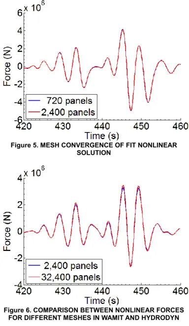
Fi gu re 4. CO M PAR ISO N O F SUR G E NO NLINEAR F O RC E BETW EEN FI T AN D HYD RO DYN
The sea state was discretized using a constant frequency step of 0.01256637 rad/s up to a first-order cut-off frequency of 2 rad/s. To aid in the comparisons, the same amplitudes and phases for each frequency step were used in both FIT and HydroDyn.
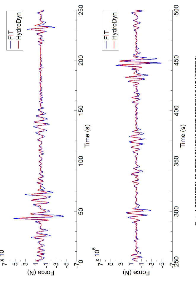
Linear Solution
The linear solution for the diffraction problem was first obtained by FIT and HydroDyn. As Fig. 3 shows, the two solutions were found to be in very good agreement. This agreement verified the accuracy of the linear solution of the FIT module, which is necessary for the computation of the nonlinear solution in the following sections.
Nonlinear Solution
Next, the nonlinear solution for the diffraction problem in the surge direction was derived using the results from the linear solution. The sum of all nonlinear loads from FIT including the Froude-Krylov impulse, the disturbance-body impulse, and the free-surface impulse was compared with the nonlinear solution obtained from HydroDyn (Fig. 4). The two solutions are in agreement, with the solution for FIT displaying a higher amplitude relative to the solution from HydroDyn. The rate of convergence is different between the two methods. The FIT formulation is a momentum method requiring only the computation of the source strengths, which are linear components, allowing the method to achieve convergence with a comparatively coarse mesh. The numerical results produced by HydroDyn in this study used a pressure integration method involving the computation of the gradient of potentials, which requires a denser mesh for convergence.
To further understand the effects of the density of the body mesh to the nonlinear solution for solving the diffraction problem using FIT, a mesh with fewer panels was also used and the solutions between a 720-panel mesh and a 2,400-panel mesh is shown in Fig. 5. The difference between the two solutions is negligible, suggesting that the solution provided by the 2,400-panel mesh is close to convergence.
A similar study on the density of the body mesh was performed for the nonlinear solution from WAMIT and the results are shown in Fig. 6. Because the solution for WAMIT is based on the pressure integration method using low-order panels, it requires many panels for convergence. As a result, a mesh with much higher density was selected for this study. A 32,400-panel mesh was chosen and the results are compared with the solution computed using 2,400 panels. The difference was found to be about 5% in amplitude, suggesting that further discretization may be needed for a converged solution. A similar finding (not shown here) resulted from comparing the diagonal (mean-drift) entries of the difference-frequency QTF using two different methods in WAMIT—the pressure integration method and the momentum conservation method. Even though the momentum conversation method converges faster than the pressure integration method in WAMIT, the momentum conservation method can only be used to compute the diagonal entries of the difference-frequency QTF, not the full difference- and sum-frequency QTFs applied here. With the pressure integration method in WAMIT, using a finer mesh near the free surface and coarser mesh elsewhere would likely lead to a converged solution faster than using a uniform fine-resolution mesh as was done here.
Figure 5. MESH CONVERGENCE OF FIT NONLINEAR SOLUTION
Figure 6. COMPARISON BETWEEN NONLINEAR FORCES FOR DIFFERENT MESHES IN WAMIT AND HYDRODYN
DISCUSSION AND CONCLUSION
A new method has been presented for evaluating the nonlinear sea-state loads on the floater of the MIT/NREL TLP wind turbine. It is based on a FIT of the loads exerted by steep ambient waves on floating bodies, which expresses the forces as the time derivatives of impulses. Explicit expressions were presented for the quadratic wave loads in terms of integrals of the velocity potentials and the source strength distribution over the body wetted surface and the internal water plane area circumventing the discretization of the infinite exterior free surface.
A comparison was carried out between the linear and second-order surge diffraction force on the MIT/NREL TLP floater between FAST’s HydroDynmodule (based on WAMIT output) and FIT. Agreement was found and the differences remaining are still being assessed. The convergence properties of the quadratic loads computed by FIT with increasing panel density were also studied and found to be excellent.
The FIT method can be used for the computation of the nonlinear loads, including slow-drift, springing, and ringing excitation and responses of floating wind turbines. It can also
be used for the evaluation of the corresponding loads and responses of ships and oil and gas platforms.
ACKNOWLEDGMENTS
The authors would like to acknowledge the support from the Massachusetts Clean Energy Center. This work was supported by the U.S. Department of Energy under Contract No. DE-AC36-08GO28308 with the National Renewable Energy Laboratory. Funding for the work was provided by the DOE Office of Energy Efficiency and Renewable Energy, Wind and Water Power Technologies Office.
REFERENCES
[1] Wayman, E. N., Sclavounos, P. D., Butterfield, S., Jonkman, J. and Musial, W., 2006. ―Coupled Dynamic Modeling of Floating Wind Turbine Systems.‖ Presented at the Offshore Technology Conference (OTC), Houston, TX, May 1–4. [2] Sclavounos, P.D., Lee, S., DiPietro, J., Potenza, G., Caramuscio, P., and De Michele G., 2010. ―Floating Offshore Wind Turbines: Tension Leg Platform and Taught Leg Buoy Concepts Supporting 3-5 MW Wind Turbines.‖ Presented at the European Wind Energy Conference EWEC 2010, Warsaw, Poland, April 20–23.
[3] Bachynski, E.E., Etemaddar, M., Kvittem, M., Luan, C., and Moan, T., 2013. ―Dynamic Analysis of Floating Wind Turbines During Pitch Actuator Fault, Grid Loss and Shutdown.‖ Energy Procedia, 35, pp. 210–222.
[4] Nielsen, F.G., Hanson, T., and Skaare, B., 2006. ―Integrated Dynamic Analysis of Floating Offshore Wind Turbines,‖ OMAE 2006, Hamburg, Germany, June 4–9.
[5] Jonkman, J., & Musial, W., 2010. Offshore Code Comparison Collaboration (OC3) for IEA Wind Task 23 Offshore Wind Technology and Deployment.
[6] Roddier, D., Cermelli, C., Aubault, A., & Weinstein, A., 2010. ―WindFloat: A floating foundation for offshore wind turbines.‖ Journal of Renewable & Sustainable Energy, 2(3), 033104.
[7] Robertson, A., Jonkman, J., Musial, W., Vorpahl, F., and Popko, W., 2014. ―Offshore Code Comparison Collaboration Continued. Phase II Results of a Floating Semi-Submersible Wind Energy System.‖ Presented at OMAE 2014, San Francisco, CA, June 8–13.
[8] Sclavounos, P.D. (2012). ―Nonlinear Impulse of Ocean Waves on Floating Bodies.‖ Journal of Fluid Mechanics, 697, pp. 316–335.
[9] Sclavounos, P.D., Forthcoming. Nonlinear Loads on Ships and Offshore Structures.
[10] Fu, S., Haase, W., Peng, S.-H., and Schwamborn, D., 2011. Progress in Hybrid RANS-LES Modelling. In Vol. 117 of Notes on Numerical Fluid Mechanics and Multi-Disciplinary Design, Springer.
[11] Stoker, J.J.,1957. Water Waves. Interscience, New York. [12] Wehausen, J.V., and Laitone, E.V., 1960. Surface Waves. In Vol. IX, Encyclopedia of Physics, pp. 446–778. Springer Verlag, New York.
[13] Jensen, J.J. (2005). ―Conditional Second-Order Short-Crested Water Waves Applied to Extreme Wave Episodes.‖ Journal of Fluid Mechanics, 545, pp. 29–40.
[14] Jonkman, J.M., Robertson, A.N., and Hayman, G.J., 2014. HydroDyn User’s Guide and Theory Manual (Draft). NREL, Golden, CO.
[15] Lee, C.-H., and Newman, J.N., 2004. ―Computation of Wave Effects Using the Panel Method.‖ In Numerical Models in Fluid-Structure Interaction, S. Chakrabarti, ed. Preprint, WIT Press, Southhampton, UK.