HAL Id: insu-01742611
https://hal-insu.archives-ouvertes.fr/insu-01742611
Submitted on 25 Mar 2018
HAL is a multi-disciplinary open access
archive for the deposit and dissemination of
sci-entific research documents, whether they are
pub-lished or not. The documents may come from
teaching and research institutions in France or
abroad, or from public or private research centers.
L’archive ouverte pluridisciplinaire HAL, est
destinée au dépôt et à la diffusion de documents
scientifiques de niveau recherche, publiés ou non,
émanant des établissements d’enseignement et de
recherche français ou étrangers, des laboratoires
publics ou privés.
simulation of 1D non-linear site effect. Results of the
validation phase
Régnier Julie, Luis-Fabian Bonilla, Pierre-Yves Bard, Hiroshi Kawase, Etienne
Bertrand, Fabrice Hollender, Marianne Marot, Déborah Sicillia, Atsudhi Nozu
To cite this version:
Régnier Julie, Luis-Fabian Bonilla, Pierre-Yves Bard, Hiroshi Kawase, Etienne Bertrand, et al..
PRENOLIN Project: a benchmark on numerical simulation of 1D non-linear site effect. Results of the
validation phase. 9ème Colloque National AFPS2015, AFPS / IFSTTAR, Nov 2015, Marne-la-Vallée,
France. �insu-01742611�
9ème Colloque National AFPS 2015 – IFSTTAR
Projet PRENOLIN banc d’essai international sur l’analyse
numérique des effets de site 1D non-linéaire. Résultat de la
phase de validation.
PRENOLIN Project:
a
benchmark
on
numerical
simulation of 1D non-linear site effect. Results of the
validation phase.
Régnier Julie * — Luis-Fabian Bonilla** — Pierre-yves Bard**,*** —Hiroshi
Kawase****— Etienne Bertrand*— Fabrice Hollender*****— Marianne Marot*—
Déborah Sicillia******— Atsudhi Nozu******
* CEREMA, Nice, France, Julie.regnier@cerema.fr ** IFSTTAR, Paris, France, fabian.bonilla @ifsttar.fr
***Univ. Grenoble Alpes, ISTerre, Grenoble, France, pierre-yves.bard@ujf-grenoble.fr ****DPRI, Kyoto, Japan, kawase.hiroshi.6x@kyoto-u.ac.jp
***** CEA, Cadarache, France, fabrice.hollender@cea.fr ******EDF, Aix-en-Provence, France, deborah.sicilia@edf.fr *******PARI, Yokosuka City, Japan, nozu@pari.go.jp.
RÉSUMÉ. L’un des objectifs du projet PRENOLIN est d’évaluer les incertitudes épistémiques associées au calcul des effets de
site 1-D non-linéaire. Le projet consiste en un banc d’essai international permettant de tester de nombreuses méthodes numériques de calcul de la réponse des sites incluant différents modèles constitutifs tenant compte du comportement non-linéaire du sol sous chargement cyclique. La phase de vérification (i.e. comparaison entre les modèles numériques et des cas canoniques) est suivie d’une phase de validation dans laquelle les résultats des approches numériques sont comparés à des enregistrements de séismes sur des sites réels bien caractérisés. 21 équipes participent au banc d’essai testant 21 codes. Les trois sites sélectionnés pour la phase de validation proviennent des réseaux accélérométriques japonais KiK-net et PARI. Les premiers résultats ont montré que le comportement non-linéaire des sols avait été sous-estimés et qu’une analyse précise et une calibration des résultats des essais en laboratoire avec des données in-situ était nécessaire. La plupart de l’incertitude épistémique provient des incertitudes sur les données d’entrées (mesure en laboratoire et interprétation) ainsi que modèle constitutif utilisé. Ce banc d’essai est conjointement financé par le projet ANR Sinaps@ et le projet SIGMA (EDF, CEA, AREVA & ENL)
ABSTRACT. One of the objectives of the PRENOLIN project is the assessment of uncertainties associated with non-linear simulation of 1D site effects. An international benchmark is underway to test several numerical codes computing the non-linear seismic site response, including various non-non-linear soil constitutive models. The preliminary verification phase (i.e. comparison between numerical codes on simple, idealistic cases) is now followed by the validation phase, which compares predictions of such numerical estimations with actual strong motion data recorded from well-known sites. The benchmark involves 21 teams dealing with 21 different non-linear computations. Extensive site characterization was performed at three sites of the Japanese KiK-net and PARI networks. The first results indicate that the linear site response is overestimated while the linear effects are underestimated. At the end of this phase, most of the epistemic uncertainty sources for non-linear site response analysis is recognized as due to the constitutive model linked to the interpretation of the soil data. PRENOLIN is part of two larger projects: SINAPS@, funded by the ANR (French National Research Agency) and SIGMA, funded by a consortium of nuclear operators (EDF, CEA, AREVA, ENL).
MOTS-CLÉS: effets de site, non-linéaire, Japon, KiKnet, modélisation numérique, validation.
KEYWORDS: Site effects, non-linear, KiK-net, numerical modelling, validation.
1. Introduction
While a consensus has undoubtedly been reached on the existence of non-linear effects, their quantification and modeling remains a challenge, despite the existence of a commonly accepted practice. The ability to accurately predict non-linear site responses has indeed already been the subject of two recent comparative tests. It was one of the targets of the pioneering blind tests initiated in the late 80's/early 90's on 2 sites of Ashigara Valley (Japan) and Turkey Flat (California); however, those sites lacked strong motion records until the 2004 Parkfield earthquake during which the Turkey Flat site experienced a 0.3g motion. A new benchmarking of 1D non-linear codes was thus carried out in the last decade. Its main findings were reported by Kwok et al., (2008) and Stewart and Kwok, 2009, who emphasized the key importance of the way these codes are used and of the required in-situ measurements. Tests on 2D NL modeling were also attempted within the framework of the Cashima/E2VP project (Bard et al 2011), but the coupling of geometrical complexity and non-linearity proved to be premature to perform such kind of computations.
For this reason, the PRENOLIN project considers only 1D soil columns, to test the non-linear codes in the simplest possible, though realistic, geometries. It is organized in two phases: (1) the initial verification phase, aiming at a cross-code comparison on very simple idealistic 1D soil columns with prescribed linear and non-linear parameters; (2) the subsequent, still ongoing, validation phase comparing numerical predictions with actual observations. The target sites are as close as possible to a 1D soil geometry (horizontal stratification), without liquefaction and associated with available sets of downhole and surface recordings for weak and very strong motions. Such pre-existing information has been complemented with careful in-situ and laboratory measurements designed as close as possible to the team requirements. The sites were selected within the Japanese KiK-net and PARI (Port and Airport Research Institute) networks.
In this article, we present the site selection and characterization, but sake of conciseness only the results of the two iterations at Sendai site are presented. The first iteration consist in forward computations without knowledge of the true surface soil response, while in the following iterations, this information was made available to the participating teams.
2. The codes tested
We compared 21 different numerical codes used by 21 participating teams; some teams tested several codes and some codes were tested by different teams: SeismoSoil (A-0), FLIP (B-0), PSNL (C-0), CYBERQUAKE (D-0), NOAH-2D (E-0), DEEPSOIL (J-0 equivalent linear method and J-1, F-0 and M-2, for the non-linear method) NL-DYAS (G-0), OPENSEES (H-0), 1DFD-NL-IM (K-0), ICFEP (L-1), FLAC.7.00 (M-0), DMOD2000 (M-1), GEFDYN (N-0), EPISPEC1D (Q-0), real ESSI (R-0), ASTER (S-0), SCOSSA-1,2 (T-0), SWAP-3C (U-0), GDNL (Y-0), SANISAND (W-0), EERA (Z-0) and PLAXIS (Z-1).
3. Site selection
Sites were selected from the KiK-net and PARI networks. The vertical accelerometric sensor array configuration sensor allowed the calculation of borehole site responses. The soil at PARI sites are less deep than the ones at the KiK-net sites, the downhole sensor is only at ~10 to 15 m depth, and a Vs profile is therefore available along the whole soil profile. More than 46,000 (six-component) recordings from KiK-net were analyzed, to derive a) the empirical site response at the 688 sites and b) the numerical linear site response from the available Vs profile. Two additional sites from the PARI network were analyzed, Sendai and Onahama (30 and 80 earthquake recordings, respectively).
9ème Colloque National AFPS 2015 – IFSTTAR 3
The site selection was performed on the basis of the following requirements: (1) availability of both strong and weak events recordings, (2) plausibility of a 1D geometrical soil configuration, i.e., satisfactory agreement between numerical and empirical site responses in the linear / weak motion range, and (3) the downhole sensor must not be too deep (depth < 250 m). To fulfill the first and second criteria, we selected sites that recorded at least two earthquakes with PGAs higher than 50 cm/s2 at the downhole sensor and we selected 1D KiK-net site configurations identified and reported by and Thompson et al., (2012), in addition to visual inspections of the comparison between the numerical and empirical site response curves. Initially, 5 KiK-net sites (FKSH14, IBRH13, IWTH04, KSRH10 and NIGH13) and 2 PARI sites were selected. Among the KiK-net sites, 4 sites were removed due to liquefaction susceptibility (FKSH14), rocky geology (IBRH13), mountainous environment (IWTH04) and insufficient nonlinearity (NIGH13). We selected 3 sites among the remaining ones -KSRH10, Onahama and Sendai - to be fully characterized for the purpose of the validation phase.
4. Site characterization and soil column definition
An extensive measurement campaign was carried out at each of these 3 sites, to obtain the in-situ VS, VP and
density profiles (using suspension logging for KSRH10 and downhole PS logging for Onahama and Sendai). Additional MASW measurements were performed to check the spatial variability of the soil properties. To constrain the non-linear soil parameters, multiple laboratory measurements were conducted on (1) Disturbed soil samples: Moisture content, soil particle density, particle size distribution, liquid and plastic limits and (2) Undisturbed soil samples: Wet density, tri-axial compression test (either drained for sandy soil or un-drained for clayey soil), consolidation tests, cyclic undrained tri-axial test for sandy samples and cyclic tri-axial test to obtain the non-linear soil properties. The number and location of the undisturbed soil samples is specified in Table 1, along with the downhole sensor depth, the maximal depth of impedance contrast and the type of soil.
Table 1. Geological characteristics of the 3 selected sites with locations of the undisturbed soil samples.
Site Downhole
sensor depth (m)
Max. impedance
contrast depth (m) Type of soil Number of cyclic tri-axial test (location)
Sendai 8 7 Sand 2 (3.3 & 5.4 m)
Onahama 11 17 Sand 3 (4.5, 7.5 &11.4 m)
KSRH10 250 44 Sand /clay 6 (3.5, 7.5, 14.5, 22.5, 29,7 & 34 m) These data, together with the observed linear empirical site response, were used by the organizing team to define a soil column to be used by all participants in the first iteration of the validation phase. At the Onahama site, it turned out that the distance between the location of the accelerometric sensors and the complementary drillings was too large compared to the strong spatial variability of the shallow soil parameters. For the second iteration
at Sendai site only, two additional soil columns were defined (SC1 and SC2). SC2 is close to the soil column of
the first iteration but with a larger low strain damping, while SC1 involves a similar Vs profile but with largely modified degradation curves adapted from the literature. In addition, the teams could volunteer to perform additional optional calculations on a preferred soil column (SCE, self defined), with either total or effective stress analysis.
The characteristic of the soil column for the iteration 1 at KSRH10 and iteration2 at Sendai site are synthesized in the table 2 and represented in figure 1.
Table 2. Soil properties of Sendai (a) and KSRH10 (b) sites.
(a)
(b)
9ème Colloque National AFPS 2015 – IFSTTAR 5
(b)
Figure 1. Vs profiles, G/Gmax and damping curves relative to shear strain, at Sendai (a) and KSRH10 (b) sites.
5. Input motion selection
The PGA and the frequency content of a recording are two relevant parameters of the input motion for describing the expected degree of non-linear soil behavior (Assimaki and Li, 2012). Nine input motions per site were selected, representing 3 different PGA levels (≥ 0.6, 0.2-0.3 m/s2 and ≤ 0.1 m/s2 at the downhole sensor) and approximately 3 distinct frequency contents. PGA was calculated on the acceleration time histories as the quadratic mean of the EW and NS components, filtered between 0.1 and 40 Hz. The numbering of input motion corresponds to decreasing PGA level from #1 to #9.
The empirical borehole Fourier transfer functions (BFSR; here, the surface to downhole motion spectral ratio) is calculated for the 18 input motions, illustrated in Figure 2. For KSRH10, the inter-event BFSR variability is quite large as well as between components of a same event. This indicates that the site does not behave similarly from one component to another and may indicate a more complex site configuration than wished. At Sendai, we observe that the BFSR of the stronger motions 1 and 2 are shifted towards lower frequencies, while their amplitude is reduced compared to the other events, reflecting non-linear soil behavior during these events
Figure 2. Comparison of the empirical transfer
functions for the EW and NS components of each of the 9 input motions for sites KSRH10 (upper graph) and Sendai (lower graph).
6. Method of analyses of the computations
The 28 team/code couples were asked to calculate the propagation of 9 input motions at both sites. They had to provide, respectively, the accelerations for 8 and 12 virtual receiver locations (at the surface and interfaces) and the stress-strain histories at 7 and 11 locations (at the middle of each soil layer).
From these results, we then performed a comparative analysis for a number of parameters:
a few engineering parameters as selected by (Anderson, 2004), i.e., PGA, response spectra at different period ranges, CAV, duration, and cross-correlation.
surface / downhole sensor amplification for Fourier (BFSRs) and response spectra
depth dependence of peak shear strain, shear strength and PGA,
G/Gmax curves, stress-strain curves at selected receivers
additional time-frequency analyses (ratio between surface and downhole Stockwell-transforms).
7. Comparison of the computations with observations
In this paper, only the results of Sendai for which two iterations have been realized are presented.
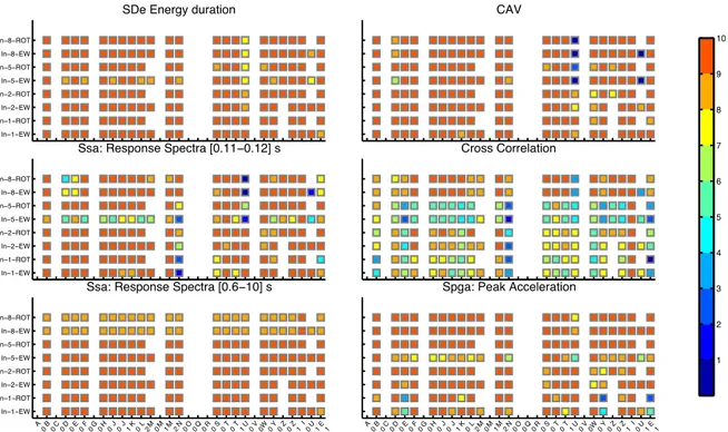
7.1. Overview of the results: Anderson criteria
The results for Anderson’s criteria (i.e comparison of each team results with empirical solution for few engineering parameters) for iterations 1 and 2 (for both SC1 and SC2 soil columns) are illustrated in Figure 5, Figure 4 and Figure 5.The results are shown only for the compulsory cases on the input motions 1, 2, 5 and 8 for both the EW and the rotated components.
The first iteration indicates a very satisfactory agreement for both the pseudo-spectral acceleration at long periods and the energy duration (as expected since the "reference" site is very shallow). Despite the very short distance between the two sensors, the cross-correlation once again proved a very stringent criterion. At short periods, the PGA is very well reproduced only for the input motions 9 and 2. For periods close to the site fundamental resonance frequency (i.e., around 8-9 Hz), there isn't any agreement on pseudo spectral acceleration, especially for input motions 1 and 5. The discrepancies between the simulations and the observation using input 1 can probably be explained by non-satisfactory non-linear soil properties. For the input 5 (a moderate motion with downhole pga around 25 cm/s2), the discrepancies are likely to be related to
specificities of the input motion. The fit significantly improved from iteration 1 to 2:
For SC2 (similar velocity profile, similar NL curves, except the increased low strain damping), the fit is clearly better for input motions 2, 5 and 8. For the input motion 5, the fit is improved when using the rotated component instead of the EW, which suggests that the EW component was not the best single component to correctly capture the down-hole reference motion. The fit remains very poor however for the strongest input motion (#1) and high-frequency indicators.
The soil column SC1, defined with non-linear soil properties imported from the literature and tuned to the observed low-strain damping, provides an additional improvement especially for the strongest input motion.
9ème Colloque National AFPS 2015 – IFSTTAR 7
Figure 3: Anderson criteria for iteration 1 at Sendai.
Figure 5: Anderson criteria iteration 2 using soil column SC1 at Sendai.
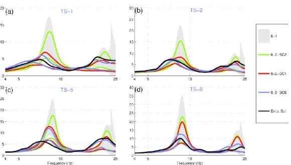
7.2. Comparing the average +/- σ of predicted response with the observed one
To compare the results of the 2 iterations and the different soil columns used, we calculated the average +/- σ of all predictions. Figure 6 represents the comparison of the empirical surface / downhole transfer function (black line) with the predictions, for the iteration 1 (grey area), the iteration 2 with the SC2 soil column (green lines), the SC1 soil column (red lines) and the preferred soil columns SCE (blue lines).
We can first observe that the variability of the computations decreases from iteration 1 to iteration 2, for all the ground motion intensity measures that are considered here.
For the input motion 8, the observation is in the prediction envelope whatever the iteration or soil column. Nevertheless, the computations get closer to the observations especially for the preferred ("SCE") soil models.
For the input motion 5, all iterations and soil columns fail to predict the observation,
For input motions 1 and 2, the results get closer to the observations from iteration 1 to 2. The fit is also significantly improved with the soil column 1 and the preferred soil column compared to the soil column 2.
9ème Colloque National AFPS 2015 – IFSTTAR 9
Figure 6: Comparison of the average +/- σ empirical transfer function (black line) with the computations, for
the iteration 1 (grey area is the ) for the iteration 2 with the SC2 soil column (green lines), the SC1 soil column (red lines) and the preferred soil columns SCE.
8. Conclusions
From the validation phase exercise at Sendai, we can observe that the fit has been significantly improved from iteration 1 to iteration 2. The exercise was blind for the first iteration, which was no longer the case for the second one. The soil parameters were adjusted to improve the fit between computations and observations, at both low and large strains. Therefore, there is no surprise for such good results at the end of the second iteration. Conversely, it was surprising (and somewhat disappointing) to observe that the fit was better using non-linear soil behavior parameters from the literature, instead of lab tests performed on specific samples from the site.
The lab measurements – as they were interpreted in July 2014 by the organizing team - appear to be insufficiently non-linear compared to the observations. The main issue concerns their relevancy (or their interpretation) at low strain, as they gave a four times smaller shear modulus than the field measurements. These lab data should have been adjusted to the in-situ measurements.
The literature curves used for this specific site gave very good results. Using such low cost characterization of the non-linear soil behavior is very attractive. It has nevertheless its own limitations: it cannot catch local site specificities and is limited to a maximum shear strain (1% for the Darendeli’s curves – a level that is however not reached in the present benchmarking exercise)
This issue on the relevance of laboratory data that represent the in-situ soil characteristics needs to be better understood. This is an ongoing investigation topic for the last months of the PRENOLIN project.
Although the epistemic uncertainty linked to the numerical approach decreases from iteration 1 to iteration 2, it is still significant and must be accounted for. When looking at the transfer functions, we observe that there is no "true" or "reference" solution valid for the whole range of frequencies and input motion levels. It is worth noticing that the observations lie within the range spanned by the whole set of computations.
The lessons of this exercise for future strong ground motion prediction exercices are multiple and declined in the following points:
For proper assessment of the non-linear site response, one should use several non-linear codes to account for the epistemic uncertainty linked to the numerical approach;
The laboratory measurements that describe the cyclic behavior must be carefully interpreted:
o Cyclic-triaxial tests cannot be considered as always fully reliable at low strains. Resonant column are an interesting complementary measurement to constrain the degradation curves at low strain. This conclusions is suggested mainly by participants coming from outside Japan, but a deeper understanding of the tri-axial test device practice in Japan should be looked for, as Japanese scientists have a long experience with Japanese measurements and do trust them even at moderate to low strains. Thus, this point is open and still under debate.
o A comparison of the results with literature curves is systematically recommended. However, there is always a possibility for non-usual soil behavior (the previous experience in Mexico City should be kept in mind)!
o Elastic properties measured in the lab should be compared to in-situ measurements.
9. Acknowledgments
We acknowledge the dedicated and proactive participating teams from all over the world: D. Assimaki, J. Shi (Caltech, US), S. Iai (DPRI, Japan), S. Kramer (Univ. Washington, US) E. Foerster (CEA, France), C. Gelis & E. Delavaux (IRSN, France), A.Giannakou (Fugro, France), G. Gazetas E. Garini & N. Gerolymos (NTUA, Greece), J. Gingery (UCSD, US), Y. Hashash & J. Harmon (Univ. Illinois, US), P. Moczo, J.Kristek & A. Richterova (CUB, Slovakia), S. Foti & S. Kontoe (Politecnico di Torino & Imperial college, Italy) G. Lanzo (Univ. Roma La Sapienza, Italy) F. Lopez-Caballero & S. Montoya-Noguera (ECP, France), F. De-Martin (BRGM, France), B.Jeremic, F. Pisano & K. Watanabe (UCD, TU Delft & Shimizu Corp, US), A. Nieto-Ferro (EDF, France), A. Chiaradonna, F. Silvestri & G. Tropeano (UNICA, Italy), MP-Santisi d'Avila (UNS, Nice) D. Mercerat (CEREMA, France) and D. Boldini (UNIBO, Italie)
10. References
Anderson, J.G., 2004. Quantitative measure of the goodness-of-fit of synthetic seismograms. 13th World Conf. Earthq. Eng. Assimaki, D., Li, W., 2012. Site and ground motion-dependent nonlinear effects in seismological model predictions. Soil Dyn.
Earthq. Eng. 143–151.
Kwok, A.O., Stewart, J.P., Hashash, Y.M., 2008. Nonlinear ground-response analysis of Turkey Flat shallow stiff-soil site to strong ground motion. Bull. Seismol. Soc. Am. 98, 331–343.
Regnier, J., 2013. Variabilité de la réponse sismique: de la classification des sites au comportement non-linéaire des sols. Paris Est.
Stewart, J., Kwok, A., 2009. Nonlinear Seismic Ground Response Analysis: Protocols and VerificaBon Against Array Data. PEER Annu. Meet. San Franc.-Present. 84.
Thompson, E.M., Baise, L.G., Tanaka, Y., Kayen, R.E., 2012. A taxonomy of site response complexity. Soil Dyn. Earthq. Eng. 41, 32–43.