Design and implementation of Carbon Monoxide and Oxygen emissions measurement in swirl-stabilized oxy-fuel combustion

(1)

Design and Implementation of Carbon Monoxide and

Oxygen Emissions Measurement in Swirl-Stabilized

Oxy-Fuel Combustion

by

Andrew Sommer Submitted to the

Department of Mechanical Engineering

in Partial Fulfillment of the Requirements for the Degree of

ARCHIVE!

Bachelor of Science in Mechanical Engineering at the

Massachusetts Institute of Technology June 2013

MA SSCH STTS INSTITlUTE

JUL 3

1 2013

L

RPARIES

Signature of

A uth o r... ...

Department of Mechanical Engineering May 10, 2013

Certified

b y ... . . . .. .. .. ...

Ronald C. Crane (1972) Professor oMechanical Engineering Thesis Supervisor

Accepted

by ... n...!... ...

Anette Hosoi Professor of Mechanical Engineering

(2)

(3)

Design and Implementation of Carbon Monoxide and

Oxygen Emissions Measurement in Swirl-Stabilized

Oxy-Fuel Combustion

by

Andrew Sommer

Submitted to the Department of Mechanical Engineering on 5/10/2013 in Partial Fulfillment of the

Requirements for the Degree of

Bachelor of Science in Mechanical Engineering

Abstract

Oxy-fuel combustion in natural gas power generation is a technology of growing interest as it provides the most efficient means of carbon capture. Since all the emissions from these power plants are sequestered, there are stringent regulations on the proportions of oxidizable contents in the flue gases. This work investigates natural gas oxy-fuel combustion and

represents the first iteration of carbon monoxide and oxygen emissions measurement in hot flue gases in the swirl-stabilized combustor at the MIT Reactive Gas Dynamics Laboratory. An equilibrium model using CANTERA was provided estimates for the experimental observations and was used to determine the accuracy of the measurement system. A water-quenched probe was designed and built to cool the sample gas and to allow measurements using a commercially available Lancom gas analyzer. Modifications to the existing combustion setup were made to facilitate emissions measurement at a sampling duct located downstream of the combustion

chamber. Measurements for comparison between air and oxy fuel combustion were done at a constant adiabatic flame temperature. This corresponds to an equivalence ratio of 0.6 for air, and a CO2 mole fraction of 0.69 for oxy-fuel combustion. Overall the measurement system

provided reasonable readings for air-combustion, but measurements in oxy-fuel combustion understated the expected CO concentrations by a factor of four and overstated expected 02

(4)

values by an order of magnitude. Air leakage into the combustion chamber is the suspected reason for these discrepancies, and recommendations are laid out for the next iteration of emissions measurement.

Thesis Supervisor: Ahmed F. Ghoniem

(5)

Acknowledgements

I would first like to thank Professor Ghoniem for giving me the opportunity to work with

his research team. I have been honored by the opportunity as an undergraduate to do complex technical work in the field of combustion and fascinated by the challenges that have been presented. I would also like to thank Dr. Santosh Shanbhogue, who was a mentor and guide during my work with the Reactive Gas Dynamics Lab. He provided invaluable assistance and advice during each aspect of my project and has taught me many lessons. Finally, I would like to thank the other members of the Reactive Gas Dynamics Lab for the work that laid the foundation for my research.

(6)

(7)

List of Figures

1-1 Air Com bustion Adiabatic Flam e M odel ... 11

1-2 Air Com bustion Em issions M odel ... 11

1-3 CO2 Em issions in Air Com bustion ... 12

1-4 Oxy-Fuel Com bustion Adiabatic Flam e M odel ... 13

1-5 Oxy-Fuel Com bustion Em issions M odel ... 14

2-1 Com bustor Graphic ... 15

2-2 Sw irlers ... 16

2-3 Exhaust Hood ... 16

2-4 W ater-Quenched Probe ... 17

2-5 Lancom 4 Gas Analyzer ... 17

2-6 Probe Design ... 18

2-7 Probe Tip Exploded View ... 19

2-8 Probe Rear ... 19

2-9 Epoxy-Sealed Hose Fittings ... 20

2-10 Probe Tip Elbow ... 21

2-11 Probe M ounted in Com bustor ... 21

2-12 Forces on the Sam pling Duct ... 22

2-13 Sam pling Duct Support Design ... 23

2-14 Sam pling Duct Support ... 24

2-15 Lancom Air Readings ... 25

3-1 Air Com bustion Em issions M easurem ent ... 27

3-2 Oxy-Fuel Combustion Emissions Measurement, 450 Swirler ... 28

3-3 Oxy-Fuel Combustion Emissions Measurement, 150 Swirler ... 29

(9)

Section 1 - Introduction

1.1 Oxy-Fuel Combustion as a Method of Carbon Sequestration

Carbon dioxide is increasingly seen as a factor in global climate change. As the world's energy needs continue to grow, the amount of carbon dioxide released through the combustion of fossil fuels will also increase. Carbon dioxide sequestration is seen as a viable means of reducing the volume of CO2 released into the atmosphere. Three methods exist for carbon capture and sequestration: 1) carbon dioxide can be separated from exhaust gases after the combustion process; 2) an integrated gasification combined cycle can be used to separate carbon products prior to combustion; 3) oxy-fuel combustion, or the burning of fuel with pure oxygen, diluted with CO2, allows for the easy capture of CO 2 after the combustion process. Of

the three paths, oxy-fuel combustion has the fewest penalties to efficiency, making it a promising candidate for adoption.

Before oxy-fuel combustion can be implemented on a broad scale, the emissions characteristics of oxy-fuel flames have to be studied. In particular, carbon monoxide and oxygen emissions from fuel combustion must meet pipeline specifications in order for oxy-fuel combustion to be adopted. Any oxidizable species present in the stream to be sequestered poses a danger to the sequestration well and is tightly regulated.[9]

Traditionally oxy-fuel combustion has been associated with coal-fueled combustion due to its high CO 2 emissions (roughly three times greater per unit of energy than natural gas

generation), but the economic and environmental advantages promised by oxy-fuel combustion are beginning to draw interest to natural gas power generation as well. Kluger describes several pilot programs at Alstom including not only a 30 MW coal oxy-fuel combustion pilot plant but also a 30 MW natural gas oxy-fuel combustion plant.[5] The economic incentives matched with the feasibility of the technology make oxy-fuel combustion an object of legitimate and valuable study.

This work will focus specifically on oxy-fuel combustion as it relates to natural gas-fueled combustors, as this is an area that has been less explored than coal applications of oxy-fuel combustion but which has increasing relevance amidst recent dramatic increases in shale gas

(10)

1.2 Prior Works

Experimental studies and modeling examining the applications of oxy-fuel combustion in natural gas turbines have been relatively absent until recently. Williams et al. examined combustion in both air and oxy-fuel on a small premixed swirl-stabilized combustor, determining that oxy-fuel equivalence ratios must be greater than 0.95 in order to produce significant CO emissions, however from that point forward those emissions rise more rapidly in oxy-fuel mixtures than in air.[10] Amato et al. used a similar combustor system along with numerical modeling to examine the relations between CO and 02 emissions and stoichiometric ratios, flame temperature, and pressure. Additionally, they found that operating at a fixed residence time reduces the emissions sensitivity of CO and 02 to flame temperature.[2] At the Reactive Gas Dynamic Laboratory at MIT, Shroll performed extensive numerical modeling of a

1-D strained flame, demonstrating that competition for the H radical caused by the presence of CO2 in oxy-fuel combustion causes elevated CO emissions.[8]

Others have examined the effect of swirler geometry on flame characteristics and emissions. Li and Gutmark correlated larger recirculation zones caused by swirl to lower temperature distributions and NOx emissions for low inlet-temperature air combustion.[6] Andrews and Ahmad determined that swirlers with a large central hub created a recirculation zone at the hottest part of the flame, increasing NOx emissions for air combustion.[3] Foley et al. examined swirling, lean, premixed air combustion, identifying four basic flame configurations at various equivalence ratios that influence recirculation and residence time.[4] Clearly there is a connection between flame behavior, residence time, temperature, and emissions. Work relating emissions in oxy-fuel combustion to swirl number is lacking from the current literature, however. This thesis seeks to take the first steps towards measuring and characterizing those relationships.

1.3 Experimental Goals

The end goal of this research is to develop a relationship between swirl number and emissions. Namely, it is expected that as swirl increases the effective residence time of the products will increase and CO emissions will decrease since the decomposition reaction has time to run its course. The goal of this thesis is to develop the first iteration of an emissions measurement system, compare it to target values developed through numerical models, and identify design changes in the experimental setup that will allow more accurate emissions measurements at a time scale that can detect the contributions of a swirler to residence time.

(11)

1.4 Numerical Modeling

Numerical modeling for this work was done using CANTERA, a package for performing thermodynamic, kinetic, and transport calculations. This package includes the GRI-Mech 3.0 optimized mechanism for performing simulations on natural gas combustion which includes 53 chemical species and 325 related reactions [1]. By equilibrating a given mixture of products and holding enthalpy and pressure constant, the adiabatic flame temperature and product concentration could be calculated. Appendix section A2 shows the exact MATLAB code used to run the simulations. Lean combustion in air can be simulated by inputting the following reactants into GRI Mech 3.0:

0 CH4 + 2 02 + 7.52 N2 (1-1)

Prior to examining species, a relationship between fuel equivalence ratio and adiabatic flame temperature is established, as shown in Figure 1-1.

E CU, -o CU 2400 2200 2000 1800 1600 1400 1200 0. 4 0.5 0.6 0.7 0.8 Equivalence Ratio' 0.9 1

Figure 1-1. As fuel equivalence ratio (0) increases, so does adiabatic flame temperature.

As a point of reference, the adiabatic flame temperature at 0=0.6 is 1666K.

This temperature relation provides a foundation upon which to perform a species analysis. Figure 1-2 shows the predicted equilibrium concentrations of CO and 02 over the same span of fuel-air equivalence ratios for air - methane combustion.

(12)

10 13 10 E CL10 2 0 0 2 S10 C 00 0 -1 10 14 12 8 -8 4 ppm CO _%02 0.4 0.5 0.6 0.7 0.8 0.9 1 Equivalence Ratio'

Figure 1-2. Predicted equilibrium CO and 02 concentrations for combustion given equivalence ratios.

in air at

Note that for 0=0.6 the predicted concentrations of CO and 02 are 9.7 ppm and 7.8% respectively. CO2 is another byproduct of air combustion, and also varies with fuel-air equivalence ratio, as shown in Figure 1-3.

9 8.5 8 7.5 0 *.6: 7 CU 6.5 5 6 05.5 5 4.5 0.4 0.5 0.6 0.7 0.8 0.9 Equivalence Ratio'

Figure 1-3. Predicted equilibrium CO2 concentration for combustion

equivalence ratios. 1 in air at given r r 2 0

(13)

The predicted CO2concentration at 0=0.6 is 5.9%.

Simulations were then run for oxy-fuel mixtures using the following reactants:

1 CH₄_{+202 + n CO}₂ The mole fraction of CO2 is defined as:

X = n n C0 2

fCH₄+n02+nCO₂ 3_+nCO2

Again, an adiabatic flame temperature relation is first established, as shown in Figure 1-4.

F-E

0 2600 2400 2200 2000 1800 1600 1400 1200 0.5 0.6 0.7 0.8 Mole Fraction CO 2 (1-2) (1-3) 0.9

Figure 1-4. Adiabatic flame temperature decreases as mole fraction of the diluent CO2

increases.

As the reactant concentration of the diluent CO2 increases the adiabatic decreases, as expected. As a reference point for oxy-fuel combustion, at x flame temperature is 1883 K. Species analysis over the same range of provides equilibrium concentrations of CO and 02 as shown in Figure 1-5.

flame temperature

=0.69 the adiabatic CO2 mole fractions

(14)

105 E CD_ 4 S 10 0 3 C- 10

0

10 2 3.5 3 0.5 AU 0.5 0.55 0.6 0.65 0.7 0.75 0.8 0.85 0.9 Mole Fraction _C02

Figurel-5. Predicted equilibrium CO and 02 Concentrations for oxy-fuel combustion at given mole fractions of C0 2.

Note that for x=0.69 the predicted concentrations of CO and 02 are 6520 ppm and 0.33%

respectively. Note also that CO emission concentrations are considerable higher for oxy-fuel combustion than for air combustion, while 02 concentrations are considerable smaller in oxy-fuel combustion.

Numerical models of air and oxy-fuel combustion provide a foundation upon which to perform experimentation and measurement of emission concentrations. The reference values

(0.6 equivalence ratio in air-combustion and 0.69 mole fraction CO 2 in oxy-fuel combustion) are the values at which measurement tests were run (as described in Section 2). Emissions concentration measurements will then be compared to the reference values to determine the validity of the measurements, to evaluate the design of the combustor setup, and to provide insight into the real behaviors observed during the experimentation.

- ppm CO * % 02 2.5 -. 2 0 -1.5 0

(15)

Section

2 -

Experimental Setup

2.1 Combustor Setup

Experiments were conducted in an axisymmetric swirl-stabilized combustor, as shown in Figure 2-1. This setup is designed for both air and oxy-fuel combustion. The premixing chamber consists of a 38mm diameter stainless-steel 316 inlet pipe with inlets for air, oxygen, carbon dioxide, and methane. All gases are metered using Sierra Instruments Smart-Trak 2 digital mass flow controllers (Model C100M-NR-3-OV1-SV1-PV2-V1-S1-C10-GS for methane, Model C100H2-NR-17-OV1-SV1-PV2-V1-S1-C10 for all other gases). For air combustion the 02 and CO2 inlets

were switched off, and for oxy-fuel combustion the air inlet was switched off. The mixture enters the combustion chamber via a choke plate, which is located 550 mm upstream of the dump plane. The mixture flows through an axial vane swirler, located 50 mm upstream of the dump plane, and is ignited using an automotive spark igniter housed 30 mm upstream of the dump plane. Two axial swirlers were used in the experiment which had vane angles of 150 and

450 respectively, as shown in Figure 2-2. A 76 mm l.D., 400 mm long quartz tube is mounted

downstream of the dump plane to allow observation of the flame. Ceramic sheet insulation was used to make O-rings at both ends of the quartz tube to provide a seal and also protect the tube from chipping.

Air/CO2 Oxygen CH4 Choke Igniter Dump/ Sampling

Inlet Plate . Expansion

Inlet Inlet Swirler Plane rucI

M

(16)

Figure 2-2. Left: The 150 axial vane swirler installed inside the combustor. Right: The 450

axial vane swirler. The white powder is aluminum oxide from another experiment running on the same setup.

The quartz tube is held in place downstream using a stainless steel circular duct 165 mm long. This duct is designed with four port taps that are used for temperature, dynamic pressure and species sampling measurements. Where this duct terminates downstream, a stainless steel exhaust hood 290 mm in diameter receives the flue gases which flow to the building exhaust trench, as shown in Figure 2-3.

Figure 2-3. Exhaust gas flows into the hood and is piped safely to an exhaust trench.

A gas sample for measuring carbon monoxide, oxygen, and carbon dioxide is extracted

using a custom designed water-quenched probe (Figure 2-4, detailed in section 2.2) connected to a Lancom 4 Portable Gas Analyzer (Figure 2-5) by a 3 meter long sample line. The gas temperature is measured using an OMEGA K-type thermocouple (Part# KTXL-116G-12).

(17)

Figure 2-4. Lancom standard probe encased in concentric tube heat exchanger

Figure 2-5. Lancom 4 Portable Gas Analyzer

Before each test, a zero calibration was performed on the Lancom gas analyzer. In this test, the analyzer draws a sample of ambient air (79% N2 and 21%02) from the surroundings through a vent in the plumbing, bypassing the probe and sample line and flowing directly over the sensors. This ensures a proper baseline for each test and eliminates sensor drift. In addition, span calibrations for each gas sensor had been run by the manufacturer to ensure accuracy over each sensor's range (see appendix Al for details on sensor range).

2.2 Designing the Water Quenched Probe

The standard sampling probe provided by the manufacturer consists of a stainless steel tube 305 mm long connected to a thermocouple sensor and a gas hose 3 m long that feeds the gas sample to the gas analyzer. This probe is rated to 600 *C. However, the temperature of the flue gases can reach up to 2000 *C. Additionally, reactions involving pollutants such as carbon monoxide would continue to run at high temperatures, and concentrations measured at the gas analyzer would be different than gas concentrations at the sampling duct due to the long

(18)

residence time. A heat exchanger was therefore required to quench the gas as it entered the probe and freeze the products at their sampling duct concentrations. As part of this thesis a design was conceived, built, and tested which provided a 3 gallon per minute flow of cold water along the gas probe, resulting in cooling of the gas by as much as 850 0_C.

This quenching was achieved by encasing the standard Lancom probe in a concentric heat exchanger consisting of two stainless steel pipes measuring 3/8" and 3/4" NPT respectively. Cold water from the RGDL building water supply system (pressurized to 100 psi) flowed into the system along the probe's length along the outermost conduit between the 3/8" and 3/4" pipes, entered the inner conduit through perforations in the 3/8" pipe near the tip of the probe, and then returned between the 3/8" pipe and the probe pipe to the cold water return pipe (pressurized to 75 psi), drawing heat from the gas in the probe as it flowed to the analyzer and shielding the probe pipe from the hot exhaust gases inside the combustor. Figure

2-6 shows the design in more detail.

Sample Gas

Cold Water Outlet Cold Water Inlet

Figure 2-6. The Lancom probe encased in a concentric heat exchanger. Cold water flows down the outer conduit and back through the inner conduit, cooling the gas as it flows inside the probe.

The water supply in the RGDL was pressurized to 100 psi, and this presented a major challenge in the design of the probe, as all connections had to be watertight at this pressure. At the tip of the probe, two stainless steel rods were bored and turned to create end plugs. Heavy interference fits (diameter overlap of 0.003") were used to eliminate the need for fittings while maintaining pressure integrity (Figure 2-7).

(19)

00

Figure 2-7. Two stainless steel end plugs were made to seal the tip of the probe.

Interference fits maintained pressure integrity against the 100 psi cold water flow.

At the back end of the probe, two stainless steel threaded caps (3/4 NPT and 3/8 NPT respectively) were used to create the seal. Each cap was through-drilled in a lathe to create a hole for the inner piping to fit through it. These holes also utilized interference fits with the inner pipes to create a seal (Figure 2-8).

Figure 2-8. Two end caps seal off the water conduits at the back end of the probe. Holes in the cap allow the inner piping to protrude past. Interference fits provide a seal.

Since all components (inner probe, both pipes, plugs, and end caps) were made of Type 304 stainless steel, they exhibit the same amount of thermal expansion when heated, so the interference fits remain intact in the heat of combustion. In contrast to the plugs in the tip of the probe, the caps' thin walls prevented the interference fit from providing a complete seal. When pressurized to 100 psi, slow leaks appeared at the back end of the probe. Loctite* Multi-Purpose Repair Putty was used to seal the leaks - the epoxy putty could be pressed into threads and gaps and provided a strong, waterproof seal when it cured. Additional leaks were fixed by

(20)

/2" inner diameter high-pressure flexible PVC tubing (two hoses, each measuring 3.8 m

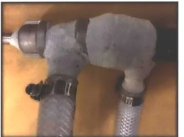
long) was chosen in order to supply the probe with water without creating a large pressure drop. Y2" to 3/8" Acetal barbed couplings were modified on the lathe (the 3/8" barb was removed) and pressed into holes milled in the pipes to create the water inlet and outlet. These press-fits were reinforced with epoxy putty to provide a seal and secure the connection against the forces of pressure and general handling (Figure 2-9). The PVC hoses along with Y2" NPT-to hose barbed adapters connected the probe to the water supply and return pipes. Zip ties were used initially to secure the fittings, but these proved to be unreliable, so hose clamps were substituted instead.

Figure 2-9. Epoxy putty supports the acetal barbed fittings at the inlet and outlet of the

probe heat exchanger and seals the pipe caps from the high pressure water supply.

A flange was press-fit onto the probe to allow for secure connection to the sampling

duct. Additionally, a 10-32 threaded elbow was machined from a Y4" diameter pipe (Figure

2-10), replacing the sintered filter on the probe and increasing the inlet pressure of the gas to

increase velocity in the sample line and reduce response time of the measurements. Due to the late addition of the elbow, the probe inlet was located 28mm radially outward from the center of the exhaust pipe. This can be remedied in future tests by adding shims between the flange and the sampling duct or by moving the flange closer to the end of the probe.

(21)

Figure 2-10. The stainless steel 10-32 threaded elbow was screwed onto the end of the probe to increase sample line flow velocity. In this image it has been blackened due to oxidation by the flue gases.

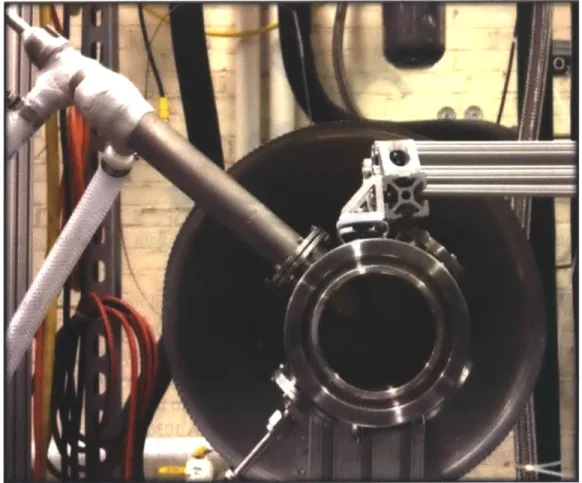
Figure 2-11 shows the fully assembled probe connected to the sampling duct.

Figure 2-11. The water-quenched probe connected to the sampling duct, as viewed axial

to the combustor.

A flow of 3 gallons per minute was observed running through the heat exchanger, as measured by a Blue-White Industries F-410 Rotameter, cooling gases by as much as 850 *C upon entering the probe.

(22)

2.3 Exhaust Sampling Duct Support

The sampling duct and probe combined weighed 3.5 kg. In addition, the hoses attached to the probe were filled with water, providing a rotational moment on the sampling duct (Figure 2-12). Alignment between the sampling duct and dump plane was crucial since the quartz tube that connected the two was fragile and would break under shear forces caused by misalignment. Additionally air influx into the combustor due to the pressure drop caused by the flame needed to be mitigated for an accurate measurement of exhaust gas. Any angular misalignment between the dump plane and sampling duct would create a gap that air could enter through.

Figure 2-12. The sampling duct support had to withstand both vertical loads and rotational moments about the axial and vertical axes.

80/20 extrusions and brackets were the primary structural materials for the sampling

duct support due to their high strength to weight ratio. Two horizontal 80/20 rails were utilized

- one directly underneath the sampling duct, the other offset beside the first. Sliders fit into the

grooves in the extrusions, allowing the sampling duct to be moved any given distance from the dump plane. Stainless steel hanging pipe supports clamped onto the sampling duct from above to prevent rotation of the sampling duct or central column. A 1030 profile column with an arc milled in the top having the same radius as the sampling duct sat below the sampling duct to take vertical loads. A second 2020 profile column riding on the offset rail with two 1010 profile arms attached to the pipe hangers controlled angle. A 1020 extrusion connected the two sliders so they would translate as one body. Figure 2-13 shows a model of the design.

(23)

Hanging Pipe Supports Offset Column Sampling Duct & Probe Central Column Slider

Figure 2-13. The central column takes the main weight of the sampling duct and probe. The hanging pipe supports take any moment that is applied and allow for angular

alignment of the front face of the sampling duct.

Considerable compliance appeared in the system, most notably at the sliders, which would rotate several degrees when a moment was applied. For this reason, the two column design was selected over a single column system. To protect against the heat of combustion, all connections between the sampling duct and support pieces utilized pieces of ceramic sheet insulation to act as heat shielding. Figure 2-14 shows the support that was built, which closely resembles the model.

The sampling duct was now able to translate freely any distance from the dump plane, free of deflections due to loading while maintaining axial alignment with the combustor and quartz tube.

(24)

Figure 2-14. The sampling duct support. Left: The sampling duct with the quartz tube in place and secured. Right: The sampling duct and support, slid closer to the dump plane to check alignment.

2.4 Emissions Measurement

Once the sampling duct was secured and the water-quenched probe was installed, the measurement process could begin. The cold water supply was turned on, the Lancom 4 Gas Analyzer was connected to the probe, and a zero recalibration cycle was run, as described in section 2.1. Once the recalibration was complete but prior to any flow in the combustor, preliminary probe readings were taken of the air in the tube to confirm proper readings at the sensor. Figure 2-15 shows the screen of the gas analyzer during this process.

(25)

--- A

Figure 2-15. "Zero" readings taken with air.

Note that some of these measurements differ from established air readings (such as 0.7 ppm

CO). This is due to sensor bias. Emissions measurements were offset by the zero bias during analysis but were corrected by subtracting this value.

With the analyzer calibrated and zeroed, emissions measurements could then be taken. Initial measurements were taken with combustion of an air-methane mix with a 450 axial vane swirler installed. The fuel - air flow was initiated and maintained at a Reynolds number of 20,000 and the concentrations were adjusted in order to reach an equivalence ratio of 0.73 at which ignition occurred. The equivalence ratio was then quickly dropped to 0.6, corresponding to an adiabatic flame temperature of 1666 K. At this point emissions logging was initiated, with manual logging being triggered every 5 seconds. The response time of the gas analyzer was roughly 15 seconds (so emissions concentrations measured at the analyzer lagged concentrations in the sampling duct by 15 seconds). The flame was maintained at an equivalence ratio of 0.6 for two minutes. Fuel flow was then shut off and the flame was extinguished, but air flow was continued in order to purge the combustor of any excess fuel and to cool the apparatus. Data logging continued at 5 seconds intervals until CO and 02

concentrations had returned to levels consistent with pure air. Multiple tests were conducted, with the analyzer recalibrated and zeroed and the combustor purged and cooled with air

(26)

Once it was confirmed that the analyzer was making accurate readings and a basis for comparison had been established from measurements taken in air, oxy-fuel experiments could be run. With the 450 axial vane swirler still installed, the analyzer was recalibrated and zeroed in air as described in the preceding paragraph. The mixed flow of carbon dioxide/oxygen/methane was then initiated and maintained at a Reynolds number of 20,000. The individual gas species concentrations were adjusted to bring the mole fraction of CO 2 to 0.69. The combustor was

promptly ignited, and data logs of the emissions concentrations were again recorded every 5 seconds. The flame was maintained for two minutes then extinguished. Fuel and oxygen flows were shut off, compressed air was turned on, and CO 2 was shut off. Flowing compressed air purged the combustor of any unburned fuel and allowed it to cool (while being significantly less expensive to run than purchased gas). Once the last test had been run and the combustor had cooled, the air flow was shut off, the 450 swirler was replaced with a 150 axial vane swirler, and the experiment was run again in the same manner.

Once all the data had been recorded and the combustor had cooled to acceptable levels, the air flow was turned off in the combustor, the flow of water through the probe's heat exchanger was shut off, and the water line was depressurized via a drain valve in the lab's piping.

Section 3 - Results and Discussion

3.1 Emissions in Air Combustion

Several emissions tests were run for combustion in air at an equivalence ratio of 0.6, as described in Section 2.4. Figure 3-1 shows the data from one such test. The flame is ignited at t=Os and extinguished at t=150s. As predicted in the numerical modeling in Section 1.4, CO 2

climbs to 6% and remains there until the flame is extinguished. Oxygen concentration drops to

9%, which is slightly higher than the expected equilibrium concentration of 7.8% that the

Cantera simulations predicted. This is likely due to an influx of ambient air into the combustion chamber downstream of the dump plane (probably at each end of the quartz tube) caused by the pressure drop induced by the flame. We also observe an initial spike in CO concentration caused by the initial combustion of excess fuel at ignition, followed by a decline to a stable equilibrium value of 10 ppm at t=90s, which approaches the equilibrium values predicted by Cantera. The CO concentration plateaus at this value until the flame is extinguished. The jump

(27)

in CO following the extinguishing of the flame is likely due to residual hydrocarbons in the flow line reacting in the hot combustion chamber following the extinguishing of the flames.

25 0 o20

0

015 0 E CL C 10 0 4-A 0 0 0 30 60 90 120 150 180 210

Time after ignition (s)

Figure 3-1. The emissions concentrations of one air combustion test, 0=0.6. CO emissions reach a stable value at t=90s and plateau until the flame is extinguished at t=150s.

The average equilibrium CO concentration for the four test runs in air was 10.22 ppm with as standard deviation of .54 ppm. This is very close to the 9.7 ppm predicted by Cantera, indicating that the reaction has approached its equilibrium value by the time it reaches the sensor.

3.2 Emissions in Oxy-Fuel Combustion

Emissions tests were then run with oxy-fuel combustion at a CO2 mole fraction of 0.69

with the 450 swirler still installed, as described in section 2.4. Figure 3-2 shows the results of one of these tests. Carbon dioxide concentrations exceed 30%, the maximum the sensor can measure, so they are not included in the figure. The oxygen concentration starts well above air concentration levels, as would be expected in oxy-fuel combustion, then drops down to 7% until the flame is extinguished. This is considerably higher than the oxygen content of 0.33%

.ppm CO S% CO2

- % 02

(28)

that is predicted by the Cantera simulations in section 1.4. Hydrocarbon emissions were measured to be less than 0.1% during combustion, indicating nearly complete product burn. This would point to the ingress of air into the combustion chamber upstream of the sampling duct due to the pressure drop caused by the flame. CO concentrations rose sharply to a plateau around 1675 ppm. 2000 1500 E 0 0 CO 0 1 1000 0

0

500 0 Figure 3 450 swir right axi 20 40 60 80 100

-2. ler S. 40 30 C 0 20 -0 0_C)4 10 IL L L .ppm CO '% ₀₂ r r 1 120 140 160

An emissions test for oxy-fuel combustion with a CO 2 mole fraction of 0.69. A

is installed. CO concentrations are on the left axis, 02 concentrations on the

The measured CO concentration at the plateau for oxy-fuel tests at a mole fraction of 0.69 and a 450 swirler was 1662 ppm with a standard deviation of 26.4 ppm.

The experiment was also run for a 15' swirler, as shown in Figure 3-3. Note that the CO concentration fluctuates more during the plateau, but that otherwise the measured emissions values are very similar between the two tests.

rr

(29)

-2000 - 1500 E 0 1000 0 0

C~)

500 0 50 100 150

Figure 3-3. An emissions test for oxy-fuel combustion with a

15* swirler is installed. 200 Sp '% - L - l Mn 250 CO2mole fraction of 0.69. A

The measured CO concentration at the plateau for oxy-fuel tests at a mole fraction of 0.69 and a 150 swirler was 1711 ppm with a standard deviation of 70.9 ppm.

Figure 3-4 compares the measured plateau CO concentrations of oxy-combustion as recorded in section 3.1. Note that oxy-fuel combustion results in CO emissions of magnitude greater than air combustion.

to those of air several orders Pm CO 02 40 30 20 10 20 . 0 0 10 c. I | 0

(30)

10 -E 0 2 0 10 a) C 0 0 C)10 100

Air, 45 Deg Swirler Oxy, 45 Deg Swirler Oxy, 15 Deg Swirler Figure 3-4. CO Emissions for air and oxy-fuel combustion. The error bars represent 2 standard deviations from the measured mean.

Both tests registered well below the predicted equilibrium CO concentration of 6520 ppm for oxy-fuel combustion at a CO2 mole fraction of 0.69. The average CO concentration with

the 45* swirler installed was 25.5% of the expected value. With the 150 swirler installed, CO emissions were 26.2% of the expected value.

It is possible that these discrepancies are due to the additional ambient air pulled into the combustor (as evidenced by the extremely high oxygen levels), diluting the exhaust gases.

CO emissions are highly sensitive to oxygen concentrations, and even small volumes of air

would decrease CO emissions substantially. Adding .1 moles of 02 and .39 moles of N2 to the

oxy-fuel reactants 1-3 (corresponding to an air leak at 5% of the inlet gas volumetric flow which is then combusted) reduces predicted CO emissions to 60% and raises 02 to 1.1%. This does not take into account additional air leaking into combustor downstream of the combustion chamber, which may or may not be burned completely but would enter the sampling duct and contribute to the measured emissions. Air-combustion measurements showed values of

C0 2+CO+0 2 above those predicted by the model. A full oxygen balance could not be performed

(31)

oxy-fuel case the CO2 levels were above the sensor's maximum range. Additionally, the analyzer

was not equipped with a N2 sensor, so measuring air leakage directly was impossible.

CO emissions are also kinetically controlled and highly dependent on temperature

history, and the reactions are occurring at temperatures less than the adiabatic flame temperature due to heat losses. This may be another reason that CO emissions are much lower than expected for oxy-fuel combustion, although it doesn't explain why 02 levels are so much higher than expected.

Section 4 -Conclusion and Recommendations

4.1 Assessment of Thesis Goals, Results

This thesis represents the first iteration of a carbon monoxide measurement system. A working system was developed to effectively measure CO and 02 emissions for both air and oxy-fuel combustion. A heat-exchanger was built that reduced sample gas temperatures by as much as 850 "C. A support was built for the sampling duct that allowed for easy mating to the

current combustor assembly. Initial measurements for air combustion indicate emissions on the order of the concentrations predicted by numerical modeling. There are however significant discrepancies between the emissions data and the models for oxy-fuel combustion. This may be due to air leakage into the combustor at both ends of the quartz tube due to the pressure drop associated with the combustion flame. Alternatively, the discrepancy in emissions may be due to temperature effects on the reactions. Additional investigation is needed into this question. There is also the question of adequate gas quenching; sample line temperatures approached

6000C as measured by the sampling probe, and CO decomposition reactions may not have been

adequately frozen in place to get a proper reading of concentrations at the sampling duct. These are the technical issues with the current experiment that must be addressed in the next iteration.

4.2 Recommendations for Future Work

In order to address the concerns mentioned, the following changes are recommended: The quartz tube should be replaced by a flanged pipe bolted and sealed to both the dump plane and sampling duct. This would eliminate air influx issues into the combustion

(32)

products and allow for more accurate measurements. If the same discrepancies in emissions were still observed, it would then be clear that they were caused by other phenomenon such as temperature variation.

A range recalibration should be conducted on the Lancom analyzer - the recommended

time between recalibrations has nearly expired.

The temperatures in the sample line need to be verified by a second thermocouple. The thermocouple installed in the probe runs axially down the length of the probe and may not accurately measure the colder temperature of the gas as it exits the probe.

If additional quenching is required, a larger diameter heat exchanger (or a longer heat

exchanger and probe) could allow further reductions in sample line temperatures.

A custom sample hose could be made with a larger inner diameter. This could increase

gas sample velocity and decrease the response time of the analyzer.

The probe inlet should be moved to the center of the sampling duct through the addition of shims or the relocation of the probe flange closer to the tip.

By solving the challenges encountered in the first iteration of the design, most notably

the issue of air leakage into the combustor, accurate emissions concentrations should be able to be measured with a higher degree of confidence, allowing a more detailed investigation into the effects of swirl number and residence time on emissions concentration.

(33)

Bibliography

[1] "Current and Future Releases of GRI-Mech." GRI-Mech. UC Berkeley. Web. 2 May 2013. <http://www.me.berkeley.edu/gri_mech/releases.htm>.

[2] Amato, A., B. Hudak, P. D'Souza, P. D'Carlo, D. Noble, D. Scarborough, J. Seitzman, and T. Lieuwen. "Measurements and analysis of CO and 02 emissions in CH 4/CO 2/02 flames." Proceedings of the Combustion Institute 33, no. 2 (2011): 3399-3405.

[3] Andrews, G. E., H. S. Alkabie, MM Abdul Aziz, US Abdul Hussain, N. A. Al Dabbagh, N. A. Ahmad, AF Ali Al Shaikly, M. Kowkabi, and A. R. Shahabadi. "High-intensity burners with low NOx emissions." Proceedings of the Institution of Mechanical Engineers, Part A: Journal of Power and Energy 206, no. 1 (1992): 3-17.

[4] Foley, C. W., I. Chterev, J. Seitzman, and T. Lieuwen. "Flame Configurations in a Lean

Premixed Dump Combustor with an Annular Swirling Flow." In 7th US National Combustion Meeting, no. 1D16. 2011.

[5] Kluger, Frank, Benedicte Prodhomme, Patrick M6nckert, Armand Levasseur, and Jean-Francois Leandri. "CO 2 capture system-Confirmation of oxy-combustion promises through pilot operation." Energy Procedia 4 (2011): 917-924.

[6] Li, Guoqiang, and Ephraim J. Gutmark. "Effects of swirler configurations on flow structures and combustion characteristics." ASME paper no. GT2004-53674, 2004.

[7] Shingley, Joseph E. Mechanical Engineering Design. 8th ed. New York: McGraw-Hill, 2011. 115-117.

[8] Shroll, Andrew P., Santosh J. Shanbhogue, and Ahmed F. Ghoniem. "Dynamic-Stability Characteristics of Premixed Methane Oxy-Combustion." Journal of engineering for gas turbines and power 134, no. 5 (2012).

[9] White, Vince, Rodney Allam, and Edwin Miller. "Purification of Oxyfuel-Derived CO2 for Sequestration or EOR." In Proceedings of the 8th Greenhouse Gas Technologies Conference GHGT, vol. 8. 2006.

[10] Williams, Timothy C., Christopher R. Shaddix*, and Robert W. Schefer. "Effect of syngas composition and C0 2-diluted oxygen on performance of a premixed swirl-stabilized combustor." Combustion Science and Technology 180, no. 1 (2007): 64-88.

(34)

Appendix

Al Lancom 4 Gas Analyzer Sensor Ranges:

Sensor 02 CO (low) CO (H, compensated) CO (high) SO, NO NO, H2S C02 "2 Hydrocarbons (CH,) Minimum Range 0 to 25% v/v 0 to 100 ppm 0 to 100 ppm 0 to 4000 ppm 0 to 100 ppm 0 to 100 ppm 0 to 100 ppm 0 to 200 ppm 0 to 25% v/v Maximum. Range* 0 to 30% v/v 0 to 6000 ppm 0 to 4000 ppm 0 to 10 % 0 to 4000 ppm 0 to 5000 ppm 0 to 1000 ppm 0 to 1000 ppm 0 to 4% v/v (Calibrated as methane) Accuracy % of range A1% A12%* +A2%* A:2%* A+2%* A2%* A2%* A2%* +A2%* Resolution 0.1% v/v 0.1 ppm 0.1 ppm 0.1 ppm 0.1 ppm 0.1 ppm 0.1 ppm 0.1 ppm 0.1% v/v 0.1% v/v

A2 Cantera Modeling Code

%% Cantera Numerical Modeling

%Air Combustion clear all clc phi= [.4: .05:1]; AFT=zeros(size(phi)); COConc=zeros(size(phi)); 02Conc=zeros(size(phi)); CO2Conc=zeros(size(phi)); ind=1; for p=.4:.05:1 Xl='CH4:'; X2=num2str(p); X3=', 02:2, N2:7.52'; X= [X1, X2, X3] ; gas= GR130(); set(gas, 'T', 300, 'P', oneatm, 'X', X); equilibrate(gas, 'HP'); AFT(ind)=temperature(gas); COConc(ind)=moleFraction(gas,'CO'); CO2Conc(ind)=moleFraction(gas,'CO2'); O2Conc(ind)=moleFraction(gas,'02'); ind=ind+l; end Z= [phi;AFT]; AFT1=AFT; ... ... .... ... ..... .. . .. .... ... . -- --- --- ---

(35)

-figure (1)

plot(phi,AFT1, 'bo-')

%title('Adiabatic Flame Temperature Variation, Methane-Air Mix', 'interpreter','latex','fontsize',16);

xlabel('Equivalence Ratio $$\varphi$$', 'interpreter','latex', 'fontsize',13); ylabel('Adiabatic Flame Temperature (K)','interpreter','latex','fontsize',13);

figure(2)

[AX,H1,H2]=plotyy(phi,COConc*1000000,phi,02Conc*100);

xlabel('Equivalence Ratio $$\varphi$$', 'interpreter', 'latex','fontsize',13); ylabel('CO Concentration, ppm', 'interpreter', 'latex', 'fontsize',13);

set(get(AX(2), 'Ylabel'), 'String', '$$CO_2,\ 0 2$$\ Concentration\ (\%)', 'interpreter', 'latex', 'fontsize',12)

set(H1, 'LineStyle', '-')

set(Hl,'Marker','o')

set(H2,'LineStyle','-') set(H2, 'Marker', 'x') set(AX(1), 'YScale', 'log');

set(AX(l), 'YTick', [1E-2,lE-l,1,10,100,1000,10000])

set(AX(2),'YTick', [0:.02:.14]*100)

set(AX(2),'ylim', [0 .14]*100)

1=legend('ppm $$Co$$', '$$\%\ 0_2$$', 'Location', 'North'); set(1, 'Interpreter', 'Latex');

figure(3)

plot(phi, CO2Conc*100, '

xlabel('Equivalence Ratio $$\varphi$$', 'interpreter','latex', 'fontsize',13); ylabel('$$CO_2$$ Concentration\ (\%)','interpreter','latex', 'fontsize',13);

%% Oxy-Fuel Simulations hold off A= [3:.1:12]; % C02 Concentration AFT=zeros(size(A)); COConc=zeros(size(A)); CO2Conc=zeros(size(A)); O2Conc=zeros(size(A)); ind=1; for p=3:.1:12 Xl='CH4:1, 02:2, C02:'; X2=num2str(p); X=[Xl,X2]; gas= GRI30(); set(gas, 'T', 300, 'P', oneatm, 'X', X); CO2Conc(ind)=moleFraction(gas,'CO2'); equilibrate(gas, 'HP'); AFT(ind)=temperature(gas); COConc(ind)=moleFraction(gas, 'CO'); O2Conc(ind)=moleFraction(gas,'02'); ind=ind+l; end AFT2=AFT; . . . . .......

(36)

figure (1)

plot(CO2Conc,AFT,'b.-')

%title('Adiabatic Flame Temperature Variation, Oxy-Combustion', interpreter, 'latex', 'fontsize',16);

xlabel('Mole Fraction $CO_2$','interpreter','latex','fontsize',13);

ylabel('Adiabatic Flame Temperature (K)','interpreter','latex','fontsize',13); %set(gca,'XDir','reverse')

figure (2)

cif

[AX,H1,H2]=plotyy(CO2Conc,COConc*1000000,CO2Conc,02Conc*100)

%title('Carbon Monoxide Concentration, Oxy-Combustion','interpreter', 'latex', 'fontsize',16); xlabel('Mole Fraction $CO 2$','interpreter','latex','fontsize',13);

ylabel('CO Concentration, ppm', 'interpreter','latex','fontsize',13);

set(get(AX(2),'Ylabel'),'String','$$0_2$$\ Concentration\ (\%)', 'interpreter','latex', 'fontsize',12) set(AX(1),'YScale', 'log'); set(AX(1),'YTick', [lE-2,1E-1,1,10,100,1000,1E4,lE5]) set(H1,'LineStyle','-') set(Hi,'Marker','.') set(AX(l),'ylim', [50 1E5]) set(H2,'LineStyle', '-') set(H2,'Marker','.')

1=legend('ppm $$CO$$','$$\%\ 0_2$$','Location','NorthEast'); set(1,'Interpreter','Latex');

%set(gca, 'XDir','reverse') %grid on

% figure(3)

% semilogy(AFT,COConc,'ko-')

% ylabel('CO Concentration, Fraction of Total', 'interpreter','latex','fontsize',13);

% xlabel('Adiabatic Flame Temperature (K)','interpreter','latex','fontsize',13);

% grid on

% title('Adiabatic Flame Temperature vs $$\varphi$$, C02 Ratio','interpreter','latex', 'fontsize',13);