HAL Id: hal-00153131
https://hal.archives-ouvertes.fr/hal-00153131
Submitted on 2 Jan 2016
HAL is a multi-disciplinary open access
archive for the deposit and dissemination of
sci-entific research documents, whether they are
pub-lished or not. The documents may come from
teaching and research institutions in France or
abroad, or from public or private research centers.
L’archive ouverte pluridisciplinaire HAL, est
destinée au dépôt et à la diffusion de documents
scientifiques de niveau recherche, publiés ou non,
émanant des établissements d’enseignement et de
recherche français ou étrangers, des laboratoires
publics ou privés.
Systematic analysis of equatorial noise below the lower
hybrid frequency.
O. Santolik, F. Nemec, K. Gereova, E. Macusova, Y. de Conchy, Nicole
Cornilleau-Wehrlin
To cite this version:
O. Santolik, F. Nemec, K. Gereova, E. Macusova, Y. de Conchy, et al.. Systematic analysis of
equa-torial noise below the lower hybrid frequency.. Annales Geophysicae, European Geosciences Union,
2004, 22 (7), pp.2587-2595. �10.5194/angeo-22-2587-2004�. �hal-00153131�
SRef-ID: 1432-0576/ag/2004-22-2587 © European Geosciences Union 2004
Annales
Geophysicae
Systematic analysis of equatorial noise below the lower hybrid
frequency
O. Santol´ık1, F. Nˇemec1, K. Gereov´a1, E. Mac ´uˇsov´a1, Y. de Conchy2, and N. Cornilleau-Wehrlin3
1Faculty of Mathematics and Physics, Charles University, V Holeˇsoviˇck´ach 2, Prague, CZ-18000, Czech Republic 2LESIA/Observatoire de Paris-Meudon, F-92195, Meudon Cedex, France
3CETP/IPSL, 10/12 Avenue de L’Europe, V´elizy, F-78140, France
Received: 5 August 2003 – Revised: 24 November 2003 – Accepted: 11 December 2003 – Published: 14 July 2004 Part of Special Issue “Spatio-temporal analysis and multipoint measurements in space”
Abstract. We report results of a systematic analysis of a large number of observations of equatorial noise between the local proton cyclotron frequency and the local lower hybrid frequency. The analysis is based on the data collected by the STAFF-SA instruments on board the four Cluster spacecraft. The data set covers their first two years of measurement in the equatorial magnetosphere at radial distances between 3.9 and 5 Earth radii. Inspection of 781 perigee passages shows that the occurrence rate of equatorial noise is approximately 60%. We identify equatorial noise by selecting data with nearly linearly polarized magnetic field fluctuations. These waves are found within 10◦of the geomagnetic equator, consistent with the published past observations. Our results show that equatorial noise has the most intense magnetic field fluctua-tions among all the natural emissions in the given interval of frequencies and latitudes. Electric field fluctuations of equatorial noise are also more intense compared to the av-erage of all detected waves. Equatorial noise thus can play a non-negligible role in the dynamics of the internal magneto-sphere.
Key words. Magnetospheric physics (waves in plasma) – Space plasma physics (waves and instabilities) – Radio sci-ence (magnetospheric physics)
1 Introduction
Equatorial noise is an intense natural emission of electromag-netic plasma waves observed within a few Earth radii (RE) of
geocentric radial distance, and always recorded very close to the geomagnetic equator. Its frequency interval ranges from a few Hertz to several hundreds of Hertz. These waves were first observed by Russell et al. (1970) in the outer plasmas-phere at frequencies between twice the local proton cyclotron frequency (fH+) and half the lower hybrid frequency (flh). Correspondence to: O. Santol´ık
(ondrej.santolik@mff.cuni.cz)
The observations were made within 2◦from the equator, and the magnetic field fluctuations carried by those waves were found to be very close to the direction parallel to the static ter-restrial magnetic field (B). This observed polarization corre-sponds well to the theoretical properties of the whistler-mode waves below flh (e.g. Stix, 1992), assuming that the wave
vectors are very close to perpendicular to B.
Later observations (Gurnett, 1976; Perraut et al., 1982; Laakso et al., 1990; Kasahara et al., 1994; Andr´e et al., 2002) revealed that the equatorial noise occurs at radial dis-tances between 2 and 7 RE, and at latitudes within 10◦from
the magnetic equator, and that its lowest frequency could go down to the fundamental fH+. Detailed time-frequency
spectrograms (Gurnett, 1976) also showed that, what ap-pears as a noise band in the low resolution data, is in fact a superposition of many spectral lines with different fre-quency spacings. The term “equatorial noise” is, however, still used even for these discrete wave phenomena, to indi-cate the connection to the original observations of Russell et al. (1970). The generation mechanism of these waves is most probably connected to the ion-cyclotron harmonic interac-tion (Gurnett, 1976), with energetic protons having ring-like distribution functions at a pitch angle of 90◦(Perraut et al., 1982). After being generated at the ion Bernstein wave-mode branches, the waves subsequently propagate in the electro-magnetic whistler mode (also known as the extraordinary or fast magnetosonic mode). Equatorial noise thus can be ob-served far away from its generation region.
Multipoint observations of equatorial noise by the four Cluster spacecraft have been presented by Cornilleau-Wehrlin et al. (2003) and Santol´ık et al. (2002). They ad-dressed the location of noise with respect to the equatorial plane and the spatio-temporal structure of its frequency spec-tra. Santol´ık et al. (2002) found these waves within 2◦of the magnetic equator, and Cornilleau-Wehrlin et al. (2003), in another case, at about 3◦of the model equator, with an exten-sion of 0.15 REin the direction perpendicular to the ecliptics.
Since a common feature of the equatorial noise is the pres-ence of harmonic lines whose spacings do not match the local
2588 O. Santol´ık et al.: Systematic analysis of equatorial noise below UT: 2100 2120 2140 2200 2220 2240 R (RE): 4.60 4.46 4.38 MLat (deg): -28.29 -16.59 -4.30 MLT (h): 0.40 0.52 0.64 4.37 4.44 4.57 8.23 20.58 32.40 0.77 0.93 1.11 10-9 10-8 10-7 10-6 10-5 nT 2 Hz -1 10 100 1000 f (Hz) flh 10-8 10-7 10-6 10-5 10-4 mV 2 m -2 Hz -1 10 100 1000 f (Hz) 0.0 0.2 0.4 0.6 0.8 1.0 Ellipticity SVD 10 100 1000 f (Hz) 0.0 0.2 0.4 0.6 0.8 1.0 Planarity SVD 10 100 1000 f (Hz)
(a)
(b)
(c)
(d)
Fig. 1. Example of data collected by Cluster 4 on 17 February 2002. From the top: (a) sum of the power-spectral densities of the three
magnetic components, (b) sum of the power-spectral densities of the two electric components ; (c) ellipticity and (d) planarity are determined using the singular value decomposition of the magnetic spectral matrix. Universal time (UT) and position of the spacecraft are given on the bottom of the figure using the radial distance (R) in the Earth radii (RE), magnetic dipole latitude (MLat) in degrees, and magnetic local time
(MLT) in hours. Maximum possible value of the local lower hybrid frequency (flh) is plotted over the panels (a)–(d). The data in panels (c)
and (d) are not shown for weak signals below 10−9nT2Hz−1.
fH+, waves have to propagate in the radial direction, in order
to move through the equatorial plane to a place with a dif-ferent magnetic field strength. Santol´ık et al. (2002) showed a case where the wave propagation directions have a radial component.
This paper is also based on the data of the Cluster project. We present the first results of our systematic anal-ysis of a large number of observations of equatorial noise. These emissions are, together with the whistler mode cho-rus, among the most intense electromagnetic waves observed in the low-latitude region of the Earth’s magnetosphere, and their sensitivity to the variations of the geomagnetic activity indicates their importance for the “space weather” applica-tions, i.e. prediction of fluxes of energetic particles as a con-sequence of variations of the solar input (Andr´e et al., 2002). Therefore, we focus our attention on the probability densi-ties of the wave intensity in both electric and magnetic
com-ponents. We establish a selection criterion for recognizing the equatorial noise emissions, and compare the intensities of equatorial noise with those of other emissions in the same in-terval of frequencies and latitudes. In Sect. 2 we will present the data set and, using an example case, we will describe our analysis methods. In Sect. 3 we will show results of the sys-tematic analysis, in Sect. 4 we will discuss these results and, finally, in Sect. 5 we will present brief conclusions.
2 Data set and analysis methods
We use the data collected by the “spatiotemporal analy-sis of field fluctuations” (STAFF-SA) instruments on board the four Cluster spacecraft operated by the European Space Agency (ESA). STAFF-SA was designed for onboard calcu-lation of power-spectral densities, mutual phases, and coher-ence relations of three orthogonal magnetic components and
two electric components (Cornilleau-Wehrlin et al., 1997, 2003). The analysis is made in 27 frequency channels between 8 Hz and 4 kHz, and the instrument has several mea-surement modes. Of those, we only use the “normal mode” in the present study. This mode provides us with the full five-component analysis in the entire frequency band of the instrument. The data are analyzed on board with the time resolution of 1 s (for the power-spectral densities) or 4 s (for the phases and coherence). The results are then compressed and transmitted to the ESA receiving stations. In the sub-sequent preprocessing phase the received data are calibrated and organized in Hermitian spectral matrices 5×5, one ma-trix per frequency channel, i.e. 27 matrices every 4 s. Each spectral matrix contains the real power-spectral densities on its main diagonal and complex cross-spectral densities as its off-diagonal elements.
We have analyzed all the preprocessed data intervals where the Cluster spacecraft were close to their perigee during the first two years of operation (2001–2002). In these portions of their orbits the spacecraft scanned the low-latitude region of the Earth’s magnetosphere at all magnetic local times, and at radial distances between 3.9 and 5 RE.
The preprocessed STAFF-SA data have been organized into intervals of ≈1-hour duration, and we have selected those in-tervals where the instrument measured within ≈30◦ of the geomagnetic equator. In most cases we have joint two or three adjacent ≈1-hour intervals, to obtain a better cover-age of the equatorial region. We have worked with the data of each spacecraft separately, thus increasing the amount of data intervals entering in the statistics. Discussion of this ap-proach is presented in Sect. 4. Using that procedure, we have collected the total number of 781 data intervals of ≈1–3 h, measured in the equatorial region close to the perigee of the four Cluster spacecraft. To ensure the coherence of our re-sults and to gain experience for their reasonable interpreta-tion, we have visually inspected all the intervals before doing the subsequent computer analysis. This inspection showed that in 671 perigee cases the data were available in a re-stricted interval of latitudes within 10◦of the geomagnetic equator where we expect equatorial noise to appear. Of those cases, we have identified the presence of equatorial noise in 398 intervals (59%).
Figure 1 shows an example of those data intervals where the equatorial noise emissions were present. The measure-ments were done by Cluster 4 on 17 February 2002. The spacecraft was close to its perigee, and we show the data recorded in the low-latitude region within ±30◦of magnetic equator (magnetic latitude is determined using the dipole ap-proximation of the Earth’s magnetic field). Figures 1a and 1b represent power-spectral densities of the magnetic and elec-tric field, respectively. Equatorial noise is the intense electro-magnetic emission seen on both panels close to the center of the time interval, within a few degrees from the equator. In the frequency domain it appears as two main peaks at ≈30 Hz and ≈70 Hz. The emission is confined below the upper es-timate of the lower hybrid frequency (flh), calculated as the
geometric average of the proton and electron cyclotron
fre-quencies. To plot this estimate in Fig. 1, we use the measure-ments of the ambient magnetic field made on board (Balogh et al., 2001). It represents the true value of flh only in a
dense plasma, with the plasma frequency much larger than the electron cyclotron frequency, which is always the case in the plasmasphere.
Multidimensional measurements of electric and magnetic fields allow us to analyze polarization properties of equato-rial noise emissions. Ellipticity Lp of polarization of the magnetic field fluctuations is shown in Fig. 1c. We use the singular value decomposition technique from Eq. (13) of Santol´ık et al. (2003), defining Lp=w2/w1, where w1
and w2are the two largest singular values of the magnetic
spectral matrix. In the idealized case of exactly planar po-larization, the result represents the ratio of the lengths of the minor and major axes of the polarization ellipse. It varies between 0 (linear polarization) and 1 (circular polarization). The equatorial noise can be easily distinguished by its po-larization close to linear, as it was first described by Russell et al. (1970). Very similar results have been obtained using classical methods based on eigenvalue analysis (e.g. Samson, 1973). The abrupt change in the Lpvalues at a constant fre-quency of 62.5 Hz outside the equatorial noise emission is an instrumental effect. It is connected to the boundary between the frequency bands of the STAFF-SA instrument, where dif-ferent averaging of measured data is done during the onboard analysis.
Figure 1d represents the planarity F of the polarization of magnetic field fluctuations from Eq. (12) of Santol´ık et al. (2003). It is defined as F =1−√w3/
√
w1, where w1and w3
are, respectively, the maximum and the minimum singular values of the magnetic spectral matrix. In an idealized case of random fluctuations, F reflects the ratio of the shortest and the longest axes of the 3-D polarization ellipsoid, defined by standard deviations of magnetic noise. A value close to 0 would mean that the fluctuations appear in all three axes of the ellipsoid with the same probability, whereas a value of 1 would represent a strict confinement of the fluctuations to a single 2-D plane. Note that the boundary at 62.5 Hz seen in Fig. 1d is the same instrumental effect as described in the previous paragraph. For the equatorial noise, the value of F ≈0.8 suggests that the magnetic field fluctuates very close to a single plane, with a small fraction of random 3-D fluc-tuations. Values of F and Lp are obviously interdependent in that sense, that a given Lp sets a lower limit of possible values of F , 1−pLp≤F ≤1. On the other hand, a given F doesn’t have any implication for possible values of Lp.
3 Systematic analysis of the entire data set
The polarization analysis shown in Fig. 1 has been done with the entire data set recorded during the perigee portions of the 781 orbits of the Cluster spacecraft. We have selected the frequency channels between 8 Hz (the lowest frequency an-alyzed by the STAFF-SA instrument) and 300 Hz (the upper estimate of the maximum flh throughout the data set). This
2590 O. Santol´ık et al.: Systematic analysis of equatorial noise below -0.5 0.0 0.5 EllipticitySVD 0 1•105 2•105 3•105 4•105 5•105 6•105 N 0 2•104 4•104 6•104 NE -0.5 0.0 0.5 EllipticitySVD 0.0 0.2 0.4 0.6 0.8 1.0 NE / N
(a)
(b)
Fig. 2. Histograms of modified ellipticity LsLp (see text)
deter-mined using the singular value decomposition of the magnetic spec-tral matrix. (a) Histogram of all 1.4×10⁷time-frequency points, plotted in red with the left-hand-side vertical scale; and of selected 1.3×10⁶intense events above 10−6nT2Hz−1, plotted in blue, with the right-hand-side vertical scale. (b) Normalized histogram of the elipticity of the intense events.
means that we use only the 16 lowest frequency channels of the instrument. The analysis has been further limited to the data measured within ±30◦of magnetic latitude from the magnetic equator. If this interval of latitudes is completely covered by the data, it would, given the orbital parameters of Cluster satellites, correspond to a time interval of approx-imately 1 h and 40 min, i.e. with the 4-second time resolu-tion, to 1500 measurements. Since the selected time intervals do not always cover that total range of latitudes, the average number in our data set is ≈1100 measurements per interval. For the 781 perigee passages, we thus have the total num-ber of 16×1100×781 ≈ 1.4×10⁷time-frequency points. In these points we have analyzed measured spectral matrices which served as input data for calculations of the average power-spectral densities of the magnetic and electric fluctua-tions, ellipticity, and planarity (see Sect. 2).
Figure 2 shows histograms constructed from the obtained ellipticity values. The results are now slightly modified com-pared to the method used in Fig. 1c. The purpose is to re-flect the sense of rotation of the wave magnetic field. We
0.2 0.4 0.6 0.8 Planarity 0 1•105 2•105 3•105 4•105 N 0 5.0•103 1.0•104 1.5•104 2.0•104 2.5•104 NE 0.2 0.4 0.6 0.8 Planarity 0.0 0.2 0.4 0.6 0.8 1.0 NE / N (a) (b)
Fig. 3. Histograms of the planarity determined using the singular
value decomposition of the magnetic spectral matrix. (a) Histogram for all 1.4×10⁷time-frequency points, plotted in red with the left-hand-side vertical scale; and for selected 5.4×10⁵nearly linearly polarized events with Lp < 0.2, plotted in blue, with the
right-hand-side vertical scale. (b) A normalized histogram for the nearly linearly polarized waves.
multiply Lp by a sign coefficient Ls, which is either −1, or +1 according to the sign of the phase shift between the two components of magnetic fluctuations perpendicular to B. The value of −1 represents the left-hand polarized waves (the sense of the ion cyclotron motion) and the value of +1 represents the right-hand polarized waves, (the sense of the electron cyclotron motion). If the polarization is linear, and the corresponding phase shifts are either 0◦or ±180◦, then Lpis zero and Lsmay be defined as −1 or +1, with no effect on the resulting product LsLp. Similarly, if the polarization is close to linear, Lpis close to zero, and the influence of Ls on the result is negligible. The values LsLpof ±1 then corre-spond to exactly circular polarization (right- or left-handed), absolute values less than 1 mean elliptic polarization, and the value of zero still represents strictly linearly polarized waves. To obtain the histograms in Fig. 2, the interval h −1, +1i has been divided into 100 consecutive subintervals, and the number of cases contained in each of these subintervals has been counted. The entire data set mainly contains right-hand, nearly circularly polarized waves with some small fraction of
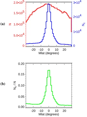
-20 -10 0 10 20 Mlat (degrees) 0 5.0•104 1.0•105 1.5•105 2.0•105 N 0 1•104 2•104 3•104 NE -20 -10 0 10 20 Mlat (degrees) 0.00 0.05 0.10 0.15 0.20 NE / N
(a)
(b)
Fig. 4. The same as in Fig. 3, but for the magnetic dipole latitude.
left-hand polarized waves (red curve in Fig. 2a). Note that the onboard compression algorithm leads to phase quantiza-tion effects reflected on the histogram as a set of superposed small-amplitude peaks. If we now select just the most in-tense waves with the magnetic spectral densities larger than 10−6nT2Hz−1, we obtain a non-negligible fraction of nearly linearly polarized waves with the absolute value of elliptic-ity below ≈0.2 (blue curve in Fig. 2a). The artifacts intro-duced by the onboard compression are removed if we cal-culate the relative fraction of the intense waves among all the recorded measurements. This normalized histogram of ellipticity (Fig. 2b) is obtained as the ratio of the blue and red histograms from Fig. 2a. It clearly shows that the ma-jority of nearly linearly polarized waves is more intense than 10−6nT2Hz−1, forming a distinct peak around zero
ellip-ticity in Fig. 2b, with a maximum close to 80%. Based on our visual inspection of all the available data from the perigee passages of the Cluster satellites, we can identify those intense linearly polarized waves with the equatorial noise emissions. As we will show next, this identification proves true, considering our results on the magnetic latitudes of these waves. From Fig. 2b we can also estimate a rea-sonable threshold of 0.2 for the ellipticity Lp, bounding the peak of the intense linearly polarized waves. This threshold will be used in the following to identify the equatorial noise emissions. -8 -6 -4 log(nT2Hz-1) 0 1•105 2•105 3•105 4•105 5•105 6•105 N 0 5.0•103 1.0•104 1.5•104 2.0•104 2.5•104 NE -8 -6 -4 log(nT2 Hz-1 ) 0.0 0.2 0.4 0.6 0.8 1.0 NE / N (a) (b)
Fig. 5. The same as in Fig. 3, but for the sum of the power-spectral
densities of the three components of magnetic field fluctuations.
Results for the planarity of the magnetic field polarization are shown in Fig. 3. We use the same analysis method as for the example case in Fig. 1d. The obtained values have been counted in 100 subintervals between 0 and 1 to construct the histograms in Fig. 3. The histogram for all events (red curve in Fig. 3a) shows a broad peak shifted toward lower values, with a maximum around 0.3. For the selected nearly linearly polarized waves with Lp< 0.2 (blue curve in Fig. 3a) the peak is clearly moved towards higher values of the planarity. Its maximum is now slightly below 0.8. As we have shown in Sect. 2, possible values of the planarity F are limited, given the ellipticity Lp. For Lp<0.2 we cannot obtain F lower than ≈0.55. Normalized histogram of the planarity values for the nearly linearly polarized waves is shown in Fig. 3b. We can see that 100% of the observations of high planarity val-ues (>0.9) correspond to the nearly linearly polarized waves. This fraction decreases toward lower planarity values down to the cutoff at F ≈0.55.
Figure 4 presents the histograms of the magnetic dipole latitudes of the events. To obtain these histograms, the in-terval from −30◦to +30◦has been divided into 50 consec-utive subintervals. The histogram for all events (red curve and left-hand scale in Fig. 4a) is not a constant function of the magnetic latitude because of the particular method we used to select the data set. Since we always selected the data intervals containing the measurements close to the magnetic
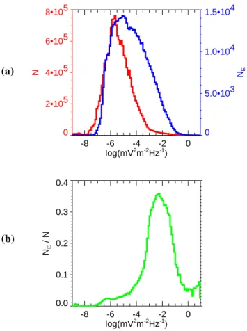
2592 O. Santol´ık et al.: Systematic analysis of equatorial noise below -8 -6 -4 -2 0 log(mV2 m-2 Hz-1 ) 0 2•105 4•105 6•105 8•105 N 0 5.0•103 1.0•104 1.5•104 NE -8 -6 -4 -2 0 log(mV2m-2Hz-1) 0.0 0.1 0.2 0.3 0.4 NE / N (a) (b)
Fig. 6. The same as in Fig. 3, but for the sum of the power-spectral
densities of the two measured components of electric field fluctua-tions.
equator, the histogram shows a broad peak centered at the zero latitude. This is therefore a purely artificial effect.
The histogram looks quite different for the waves with Lp<0.2 (blue curve and right-hand scale in Fig. 4a). The maximum is again close to the equator, but the peak is now much narrower, with the majority of events confined within 10◦of the magnetic equator. The ratio of the two histograms, shown in Fig. 4b, again forms a narrow peak, with approx-imately the same width. It moreover shows that about 17% of all events observed close to the magnetic equator is nearly linearly polarized. This fraction decreases toward higher lat-itudes. For latitudes to the south of −10◦ and to the north of +10◦, it goes down to 1–2%. This residual value will be discussed in Sect. 4. The majority of the observed nearly lin-early polarized waves is, however, cllin-early concentrated close to the equator. This further validates this selection criterion for the equatorial noise emissions.
In the analysis presented in Fig. 2 we have used a threshold of 10−6nT2Hz−1 to select intense waves. Figure 5 shows more details on the distribution of the obtained values of the magnetic power-spectral density. To construct the his-tograms, the interval between 10−10and 10−2nT2Hz−1has been divided into 100 consecutive logarithmic subintervals. The histogram of all events (red curve and left-hand scale in Fig. 5a) peaks close to 10−7nT2Hz−1, steeply decreases just
below 10−6nT2Hz−1, and forms a decreasing tail at higher
intensities.
The main peak is only slightly higher for the waves with Lp< 0.2 (blue curve and right-hand scale in Fig. 5a), but the high-intensity tail extends to significantly higher inten-sities with a higher probability. The ratio of the two his-tograms, shown in Fig. 5b, reveals that the linearly polarized waves dominate the most intense emissions with the mag-netic power-spectral density above 10−4nT2Hz−1, leaving only about 20% of those intense events to waves with a dif-ferent polarization. Oppositely, a very low relative fraction of nearly linearly polarized waves is observed for less intense waves below 10−6nT2Hz−1.
Figure 6 shows histograms of the electric power-spectral density in a similar format as in Fig. 5. We use the inter-val of inter-values between 10−9 and 101mV2m−2Hz−1, again divided into 100 consecutive logarithmic subintervals. The histogram of all events (red curve in Fig. 6a) has a peak value close to 10−5mV2m−2Hz−1, about one order of magnitude lower than the histogram for the nearly linearly polarized waves (blue curve). Above 10−4mV2m−2Hz−1, the proba-bility density for the Lp<0.2 subset of events is shifted by about two orders of magnitude higher. The relative fraction of the nearly linearly polarized waves (the ratio of the two histograms shown in Fig. 6b) doesn’t reach such as high val-ues as in the case of the magnetic field fluctuations. It shows a peak fraction of about 35% for relatively intense waves slightly below 10−2mV2m−2Hz−1, but for higher
intensi-ties the relative fraction again decreases down to about 5%. This means that other types of polarization dominate at those extremely high intensities.
4 Discussion
The most important simplification in our analysis method is the selection criterion we use to recognize the equatorial noise emissions. To analyze large volumes of data it is in-evitable to use an automatic recognition procedure, always taking the risk that some data points are either not selected when they should be, or selected by mistake. On the other hand, the advantage of this approach is that the selection is absolutely objective, based on a well-defined criterion, thus removing all possibilities for subjective case-by-case judge-ment which could bias the resulting statistics. In this study we have chosen to set up a relatively simple criterion based on the ellipticity of the magnetic field fluctuations, using known characteristics of the equatorial noise and the visual inspection of all the cases. To verify this approach we have checked the resulting statistics of magnetic latitude and pla-narity of polarization.
The only main problem of this selection criterion has been found in the analysis of magnetic latitudes (Fig. 4b). We have obtained a constant fraction of 1–2% of the nearly lin-early polarized waves for magnetic latitudes below −10◦and above +10◦. If we have no other explanation of these waves, it would mean that the linearly polarized equatorial noise
extends in latitude at least 30◦ from the magnetic equator. This would be in contradiction with the results published in the past. An alternative explanation could be that these ob-servations correspond to linearly polarized signals that we wrongly classify as equatorial noise. We suppose the phe-nomenon is connected to the low-frequency magnetic noise of the instrument. We can see in Fig. 1c that the instrumental noise creates patchy appearances of nearly linear polariza-tion well outside the compact time-frequency region of the natural equatorial noise. Since these spots of linear polar-ization are evenly distributed at all latitudes, the result is the observed 1–2% floor on the normalized histogram.
To test this hypothesis we have further narrowed our selec-tion criteria to include only the most intense waves, with the magnetic spectral density larger than 10−6nT2Hz−1. This condition has been combined with the threshold Lp<0.2. In such a way, the influence of the weak instrumental noise has been eliminated. The resulting normalized histogram (Fig. 7) proves that the main peak close to the equator remains in place as we see it in Fig. 4b but the 1–2% floor disappears. More precisely, the main peak reaches somewhat lower val-ues of ≈10%, and the fraction becomes negligible outside the interval of magnetic latitudes between −10◦and +10◦. This confirms the hypothesis that the 1–2% floor in Fig. 4b is owing to the instrumental noise.
In the present study, we have made another simplification in analyzing the data of the four Cluster spacecraft separately. The approach naturally increases the volume of data entering in the statistics by a factor of 4. However, all the spacecraft pass through the equatorial region in relatively short inter-vals of time, from less than one minute up to about 45 min, depending on the actual configuration of the spacecraft or-bits. We can then question the hypothesis of the indepen-dence of the four data sets obtained by the different space-craft. The geomagnetic conditions certainly are very similar for the four spacecraft during their closely separated perigee passages, but, nevertheless, the internal structure of the equa-torial noise emissions can be highly variable at spatiotem-poral scales comparable to the separation of the spacecraft (Santol´ık et al., 2002). In our data set we can find cases where the position of the peak intensity and the latitudinal extent of the equatorial noise are nearly the same on the four spacecraft, and other cases where these parameters are con-siderably different. Detailed analysis of these differences is beyond the scope of the present paper but for the purpose of this discussion we can conclude that the total number of in-dependent cases can be up to 4 times lower, if we consider as independent only those passages separated by at least one full orbital period of the spacecraft (2 days and 9 h). This still does not decrease the total volume of data below any reason-able limit of statistical reliability (recall that the total number of time-frequency points is 1.4×10⁷ – after using the most severe selection criteria in Fig. 7 this number still reaches a value of 2×10⁵).
The analysis of the electric and magnetic power-spectral densities is the main purpose of this work. The results show that, without any doubt, the nearly linearly polarized
emis--20
-10
0
10
20
Mlat (degrees)
0.00
0.02
0.04
0.06
0.08
0.10
0.12
N
E/ N
Fig. 7. The same as in Fig. 4b, but with the additional selection
cri-terion of the magnetic spectral density larger than 10−6nT2Hz−1.
sions are the most intense ones in the given interval of fre-quencies and latitudes, as concerns the magnetic field fluctu-ations. Electric field fluctuations of these emissions are also more intense compared to the average of all detected waves but still their relative fraction in Fig. 6b decreases at very high intensities of more than 10−2mV2m−2Hz−1. It then appears interesting to determine what kind of waves consti-tutes those in approximately 95% of the intense events. Here we must take into account that the selection criterion is based on the polarization of the magnetic fluctuations and does not take into account the polarization of the wave electric field. Intense electrostatic waves thus would not be selected even if they were linearly polarized because they are not accom-panied by a magnetic field signal. Thus, we interpret these intense waves as broadband electrostatic noise, often occur-ring at higher latitudes which are magnetically connected to the Southern and Northern auroral regions. An example can be seen in Fig. 1b where broad-band electrostatic fluctuations are mainly observed at magnetic latitudes below −25◦ and above +25◦. Projected along the approximately dipolar mag-netic field lines on the Earth’s surface, these positions cor-respond, respectively, to auroral latitudes below −65◦, and above +65◦.
The final note of this discussion concerns the significance of our results. We have proven that equatorial noise is the most intense electromagnetic emission within 30◦of the ge-omagnetic equator, in the frequency range between fH+ and flh, and in the range of radial distances between 4 and 5 RE.
As we have shown in Sect. 2, equatorial noise is detected in approximately 60% of all passages of the Cluster spacecraft through the equatorial region at 4–5 RE. This high
occur-rence rate, together with the relatively high observed intensi-ties, indicate that the importance of equatorial noise may be not as marginal, as would suggest the low number of papers
2594 O. Santol´ık et al.: Systematic analysis of equatorial noise below concerning these emissions which can be found in the public
literature. Our results suggest an analogy with natural emis-sions of whistler-mode chorus (generally observed above flh),
which are also very intense, and which are believed to signif-icantly influence the dynamics of the energetic electrons in the Earth’s outer radiation belt (Meredith et al., 2003; Horne et al., 2003; Horne and Thorne, 2003). According to the most accepted generation mechanism of equatorial noise (Gurnett, 1976; Perraut et al., 1982), its amplification is fed by the free energy in the distribution functions of energetic ions, which may be significantly influenced by interactions with these waves.
Natural emissions of equatorial noise can thus play a non-negligible role in the dynamics of the internal magneto-sphere. Equatorial noise can lead to modifications of the dis-tribution functions of energetic ions, possibly causing their perpendicular heating or, on the other hand, phase-space dif-fusion and eventual precipitation into the Earth’s atmosphere. All those arguments are, however, still rather speculative, and global effects of equatorial noise have yet to be quantitatively determined. Our results may indicate that this future research is worth being done.
5 Conclusions
We have described the first results of a systematic study of equatorial noise observed by the Cluster spacecraft between the local proton cyclotron frequency and the local lower hy-brid frequency. This study has been based on the data mea-sured by the STAFF-SA instrument during its first two years of operation. We have analyzed data collected during 781 perigee intervals of the four Cluster spacecraft at radial dis-tances between 3.9 and 5 Earth radii, and at magnetic lati-tudes between −30◦and +30◦. Inspection of these intervals has shown that the occurrence rate of equatorial noise is ap-proximately 60%.
Polarization analysis of magnetic field fluctuations has al-lowed us to select nearly linearly polarized waves with ellip-ticities below 0.2. These waves have been found to have the highest planarity among all the collected wave observations. They have been mainly found within 10◦of the geomagnetic equator. A small fraction of these waves observed at higher latitudes can be explained by the influence of instrumental noise. These results indicate, consistent with the subjective experience gained from the visual inspection of the entire data set, that the low-ellipticity criterion is able to identify equatorial noise with a reasonable success.
Equatorial noise has been shown to have the most intense magnetic field fluctuations among all the natural emissions in the given interval of frequencies and latitudes, being de-tected in approximately 80% of the cases where the mag-netic power-spectral density exceeds 10−4nT2Hz−1. Elec-tric field fluctuations of equatorial noise are more intense compared to the average of all detected waves but their rel-ative fraction decreases at very high intensities of more than
10−2mV2m−2Hz−1, owing to the 95% domination of the
broad band electrostatic noise.
The relatively high observed intensities and high occur-rence ratios of equatorial noise indicate that these natural emissions can play a role in the dynamics of energetic ions in the internal magnetosphere. More research is needed to quantify their influence.
Acknowledgements. We sincerely thank Chris Harvey of CESR
Toulouse, Michel Parrot of LPCE Orleans, Milan Maksimovic of the Meudon Observatory, and other colleagues from the STAFF team for construction, calibration and operations of the instrument and for fruitful discussions of the data. We gratefully acknowledge “space weather” discussions with Franc¸ois Lefeuvre of LPCE Or-leans, who significantly influenced the principal direction of this research. Our thanks are due to the PI of the FGM instrument (A. Balogh) for the DC magnetic field data used for reference and coordinate transformations, and to the Hungarian Cluster Data Cen-ter which provides auxiliary data. ESA and CNES are thanked for their support for the STAFF experiment. This research was sup-ported by the Czech Grant Agency grant No. 202/03/0832.
Topical Editor T. Pulkkinen thanks a referee for his help in eval-uating this paper.
References
Andr´e, R., Lefeuvre, F., Simonet, F., and Inan, U. S.: A first ap-proach to model the low-frequency wave activity in the plasmas-phere, Ann. Geophys., 20, 981–996, 2002.
Balogh, A., Carr, C. M., Acu˜na, M. H., et al.: The Cluster Magnetic Field Investigation: overview of in-flight performance and initial results, Ann. Geophys., 19, 1207–1217, 2001.
Cornilleau-Wehrlin, N., Chauveau, P., Louis, S., et al.: The Clus-ter spatio-temporal analysis of field fluctuations (STAFF) exper-iment, Space Sci. Rev., 79, 107–136, 1997.
Cornilleau-Wehrlin, N., Chanteur, G., Perraut, S., et al.: First results obtained by the Cluster STAFF experiment, Ann. Geophys., 21, 437–456, 2003.
Gurnett, D. A.: Plasma wave interactions with energetic ions near the magnetic equator, J. Geophys. Res., 81, 2765–2770, 1976. Horne, R. B., Glauert, S. A., and Thorne, R. M.: Resonant diffusion
of radiation belt electrons by whistler-mode chorus, Geophys. Res. Lett., 30, 9, 1493, doi:10.1029/2003GL016963, 2003. Horne, R. B. and Thorne, R. M.: Relativistic electron
ac-celeration and precipitation during resonant interactions with whistler-mode chorus, Geophys. Res. Lett., 30, 10, 1527, doi:10.1029/2003GL016973, 2003.
Kasahara, Y., Kenmochi, H., and Kimura, I.: Propagation charac-teristics of the ELF emissions observed by the satellite Akebono in the magnetic equatorial plane, Radio Sci., 29, 751–767, 1994. Laakso, H., Junginger, H., Roux, A., Schmidt, R., and de Villedary, C.: Magnetosonic waves above fc(H+) at geostationary orbit:
GEOS 2 results, J. Geophys. Res., 95, 10 609–10 621, 1990. Meredith, N. P., Cain, M., Horne, R. B., Thorne, R. M., Summers,
D., and Anderson, R. R.: Evidence for chorus-driven electron acceleration to relativistic energies from a survey of geomag-netically disturbed periods, J. Geophys. Res., 108, A6, 1248, doi:10.1029/2002JA009764, 2003.
Perraut, S., Roux, A., Robert, P., Gendrin, R., Sauvaud, J.-A., Bosqued, J.-M., Kremser, G., and Korth, A.: A systematic study of ULF waves above FH+ from GEOS 1 and 2 measurements
and their relationships with proton ring distributions, J. Geophys. Res., 87, 6219–6236, 1982.
Russell, C. T., Holzer, R. E., and Smith, E. J.: OGO 3 observations of ELF noise in the magnetosphere: 2. The nature of the equato-rial noise, J. Geophys. Res., 73, 755–768, 1970.
Samson, J. C.: Descriptions of the polarization states of vector pro-cesses: Applications to ULF magnetic fileds, Geophys. J. R. As-tron. Soc., 34, 403–419, 1973.
Santol´ık, O., Pickett, J. S., Gurnett, D. A., Maksimovic, M., and Cornilleau-Wehrlin, N.: Spatiotemporal variability and propaga-tion of equatorial noise observed by Cluster, J. Geophys. Res., 107, A12, 1495, doi:10.1029/2001JA009159, 2002.
Santol´ık, O., Parrot, M., and Lefeuvre, F.: Singular value decompo-sition methods for wave propagation analysis, Radio. Sci., 38, 1, 1010, doi:10.1029/2000RS002523, 2003.