Methoden
Markus Giftthaler*, Thomas Wolf, Heiko K. F. Panzer, and Boris Lohmann
Parametric Model Order Reduction of
Port-Hamiltonian Systems by Matrix Interpolation
Parametrische Modellordnungsreduktion von Port-Hamilton Systemen mittels
Matrixinterpolation
Abstract: In this paper, parametric model order
reduc-tion of linear time-invariant systems by matrix interpola-tion is adapted to large-scale systems in port-Hamiltonian form. A new weighted matrix interpolation of locally re-duced models is introre-duced in order to preserve the port-Hamiltonian structure, which guarantees the passivity and stability of the interpolated system. The performance of the new method is demonstrated by technical examples.
Keywords: Parametric model order reduction, matrix
in-terpolation, port-Hamiltonian systems.
Zusammenfassung: In diesem Beitrag wird eine
Metho-de zur parametrischen MoMetho-dellordnungsreduktion linea-rer, zeitinvarianter Systeme mittels Matrixinterpolation auf Originalsysteme in Port-Hamilton Form angepasst. Ein Vorgehen zur Matrixinterpolation, welches die Port-Hamilton Struktur im interpolierten System erhält, wird vorgestellt. Dies garantiert Passivität und Stabilität bei der parametrischen Modellordnungsreduktion. Zwei techni-sche Beispiele zeigen die Leistungsfähigkeit der neuen Me-thode.
Schlüsselwörter: Parametrische
Modellordnungsredukti-on, MatrixinterpolatiModellordnungsredukti-on, Port-Hamilton Systeme.
DOI 10.1515/auto-2013-1072
Received November 21, 2013; accepted June 23, 2014
*Corresponding author: Markus Giftthaler, Department of
Mechanical and Process Engineering, ETH Zürich, Sonneggstr. 3, CH-8092 Zürich, e-mail: [email protected]
Thomas Wolf, Heiko K. F. Panzer, Boris Lohmann: Institute
of Automatic Control, Technische Universität München, Boltzmannstr. 15, D-85748 Garching bei München
1 Introduction
The precise mathematical modeling of complex dynam-ical systems may result in systems of differential equa-tions of such a high order that their processing can become very time-consuming or even unfeasible due to shortage of RAM, which is therefore neither reasonable nor prof-itable. Model Order Reduction (MOR) addresses that prob-lem and seeks to approximate the original data of a large-scale model to a much smaller, reduced system.
Paramet-ric Model Order Reduction (pMOR) additionally tries to
pre-serve the system’s dependency on one or more parameters – for example geometric variables or material properties – within the reduced model.
One approach to describe dynamical systems, along-side the well-known first-order state-space representation, Equation (1), is the port-Hamiltonian representation. This is an energy-oriented form of system description with high physical interpretability, which additionally ensures pas-sivity. In recent years, the port-Hamiltonian representation has gradually advanced and gained importance for auto-matic control purposes [1]. Likewise, efforts for developing passivity-preserving model reduction techniques for port-Hamiltonian systems have been undertaken. For exam-ple, structure-preserving MOR approaches using moment matching were presented in [2,3]. AnH2-optimal tech-nique including tangential interpolation was suggested in [4].
In this paper, the framework for parametric model order reduction of linear time-invariant systems as pre-sented by Panzer et al. in [5] is extended to linear time-invariant (LTI) systems that are originally modeled in port-Hamiltonian form. Merging pMOR by matrix interpolation with port-Hamiltonian representation results in the advan-tage that stability is preserved in the interpolated system. In Section2, moment matching and parametric model order reduction by matrix interpolation are reviewed. The port-Hamiltonian representation is summarized in
Sec-tion3and the employed structure-preserving MOR tech-nique is presented. In Section4, methods for structure-preserving pMOR for two different representations of port-Hamiltonian systems are introduced and discussed. Two simulation examples follow in Section5.
2 Review of Projection-based MOR
and pMOR
In this section, we briefly review projection-based model order reduction and parametric model order reduction by matrix interpolation.
2.1 Order Reduction by Moment Matching
and Krylov Subspaces
Consider a linear time-invariant Multi-Input/Multi-Output (MIMO) state-space system in the form
E˙x(𝑡) = Ax(𝑡) + Bu(𝑡)
y(𝑡) = Cx(𝑡) (1) with the state vectorx ∈ ℝ𝑛, the input vectoru ∈ ℝ𝑚and the output vectory ∈ ℝ𝑙. We haveE, A ∈ ℝ𝑛×𝑛and assume thatdet E ̸= 0and thatE−1Ais Hurwitz. Furthermore we haveB ∈ ℝ𝑛×𝑚andC ∈ ℝ𝑙×𝑛. It is assumed that system (1) is both controllable and observable. The order𝑛is consid-ered to be large. Let the reduced system be
Er˙xr(𝑡) = Arxr(𝑡) + Bru(𝑡)
yr(𝑡) = Crxr(𝑡) (2)
with model order𝑞 ≪ 𝑛,xr∈ ℝ𝑞,Er, Ar∈ ℝ𝑞×𝑞,Br∈ ℝ𝑞×𝑚 andCr∈ ℝ𝑙×𝑞.
The main idea of moment matching is to expand the frequency-domain transfer functions of the original- and the reduced system in Taylor series about an expansion point𝑠0∈ ℂand match the first𝑞coefficients by means of a suitable projection: the original state vectorxis approxi-mated byx ≈ VxrwithV ∈ ℝ𝑛×𝑞and the state equation is multiplied with a suitably chosen matrixW⊤ ∈ ℝ𝑞×𝑛from the left.
A block Krylov subspace of order𝑝with respect to ma-tricesA ∈ ℝ𝑛×𝑛andR ∈ ℝ𝑛×𝑚is defined as
K𝑝(A, R) = colspan {R, AR, A2R, . . . , A𝑝−1R} (3) Remark: For the ease of presentation it is assumed that all
directions defining a block Krylov subspace (3) are linearly
independent. This implies that all block Krylov subspaces which will be employed in this work have full column rank 𝑝 ⋅ 𝑚. If the assumption does not hold, deflated block Krylov subspaces should be employed [7], which can be incorporated into the presented framework in a straight-forward way.
Lemma 1. [8]: IfVis chosen as a set of basis vectors of the block Krylov subspace
K𝑠0
𝑝 := K𝑝((A − 𝑠0E)−1E, (A − 𝑠0E)−1B) (4)
and W is arbitrary but such that Ar and Er are non-singular, the first𝑞block moments of the reduced system with Er = W⊤EV Br = W⊤B Ar= W⊤AV Cr= CV (5) match.
In this work, we calculate an orthogonal basisVof the union of different Krylov subspaces
⋃ 𝑖 ∈{1,2,...,𝑘} K𝑠𝑖 𝑝𝑖, with 𝑘 ∑ 𝑖=1𝑝𝑖⋅ 𝑚 = 𝑞 (6)
by an Arnoldi-like approach, [9]. Krylov subspace meth-ods for model order reduction are computationally fast, as the main effort is an LU-decomposition during the Arnoldi-procedure. Furthermore, a figurative interpreta-tion of the reducinterpreta-tion process is available: we can think of it as a projection from the original state space to the particu-lar subspace which is spanned byEV, using the projector
EV(W⊤EV)−1W⊤. We will denote the tall and skinny
ma-tricesVandWas projection matrices in the remainder of this paper. Drawbacks of the method are that no general error bound is known and that stability might not be pre-served in the reduced model.
2.2 Parametric Model Order Reduction by
Weighted Matrix Interpolation
If the large-scale system’s behavior additionally depends on a parameter vectorp ∈ 𝛱 ⊆ ℝ𝑑, the system matrices becomeE → E(p),A → A(p),B → B(p)andC → C(p). An exact computation of the reduced system at numerous points in the parameter space may be inefficient. The gen-eral idea of parametric model order reduction by matrix interpolation is therefore the following: given a large-scale system at𝑘sampling pointsp1,p2. . . p𝑘in the parameter
space, first reduce each system to desired order𝑞. Then, in order to approximate the parameter-dependency, the idea is to interpolate between the resulting low-order systems by Er,int= 𝑘 ∑ 𝑖=1 𝜔(p𝑖)Er,𝑖 Ar,int= 𝑘 ∑ 𝑖=1 𝜔(p𝑖)Ar,𝑖 Br,int= 𝑘 ∑ 𝑖=1𝜔(p𝑖)Br,𝑖 Cr,int = 𝑘 ∑ 𝑖=1𝜔(p𝑖)Cr,𝑖 (7)
with weighting factors𝜔(p𝑖) ∈ ℝand∑𝑘𝑖=1𝜔(p𝑖) = 1. The interpolation could also take place in nonlinear form, but for simplicity, we restrict ourselves to linear interpolation in this work.
However, a direct interpolation of reduced matrices (5) according to (7) is not meaningful since the subspaces are themselves parameter-dependent (see e. g. Equation (4)). Two state vectorsxr,1 andxr,2from different reduced sys-tems are not comparable to each other as they are located in different subspaces – except for the improbable case of matching projection matricesV1 = V2.
The direct interpolation (7) of systems that are not comparable to each other can yield e. g. singularEr,intor other unwanted effects. Therefore, it is mandatory to make the reduced system matrices compatible in some sense. As shown in [5], this can be achieved by embedding the lo-cally reduced systems into the original coordinates of the
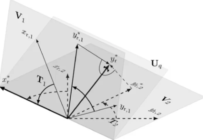
Figure 1: The process of making two pairs of basis vectors of locally
reduced systems{𝑥r,1,𝑦r,1} and {𝑥r,2,𝑦r,2} compatible with respect to a common subspaceU𝑞. The subspaceU𝑞unites the dominant directions ofV1andV2. The matricesT𝑖are chosen such that the images of corresponding pairs of basis vectors coincide after embedding them into the coordinates of the large-scale systems and a subsequent orthogonal projection intoU𝑞. In this example, 𝑥r,1and𝑥r,2are rotated such that𝑥∗r is located in in the intersection ofV1andV2. Accordingly, the images of𝑦∗r,1and𝑦r,2∗ coincide after orthogonal projection intoU𝑞.
large-scale system and subsequently orthogonally repro-jecting them into a common subspaceU𝑞. We review this approach in the remainder of this section.
The subspaceU𝑞is found using a Singular Value
De-composition (SVD)Vall= USN⊤withVall:= [V1V2. . . V𝑘] being the total of all 𝑘projection matrices and everyV𝑖 being orthogonal. By choosing the first𝑞columns ofUas basis forU𝑞, the new combined subspace unites the most dominant directions of all involved reduced systems’ sub-spaces. In this work, we assume that the SVD is solvable in a large-scale setting, given that the number of sampling points in the parameter space is small enough.
A regular state transformation
xr,𝑖= T−1𝑖 x∗r,𝑖 (8)
is applied to each of the𝑘reduced systems (wherexr,𝑖∗ de-notes a state vector in reduced and re-adjusted representa-tion) and each of these𝑘systems is multiplied with a regu-lar matrixM𝑖∈ ℝ𝑞×𝑞from the left, which leaves the input-output behavior unchanged:
E∗ r,𝑖 ⏞⏞⏞⏞⏞⏞⏞⏞⏞⏞⏞⏞⏞⏞⏞⏞⏞ M𝑖Er,𝑖T−1𝑖 ˙x∗r,𝑖= A∗ r,𝑖 ⏞⏞⏞⏞⏞⏞⏞⏞⏞⏞⏞⏞⏞⏞⏞⏞⏞ M𝑖Ar,𝑖T−1𝑖 x∗r,𝑖+ B∗ r,𝑖 ⏞⏞⏞⏞⏞⏞⏞⏞⏞⏞⏞ M𝑖Br,𝑖u yr,𝑖= C⏟⏟⏟⏟⏟⏟⏟⏟⏟⏟⏟r,𝑖T−1𝑖 C∗ r,𝑖 x∗r,𝑖 . (9)
In the following, we review how the matricesM𝑖andT𝑖 are chosen in [5] such that a weighted interpolation of the locally reduced systems becomes meaningful.
The reasoning for choosingT𝑖is as follows: consider𝑘 locally reduced systems with state vectorsx∗r,𝑖. First, reap-ply the transformation (8). Second, write everyxr,𝑖in coor-dinates of the large-scale system by multiplying it withV𝑖 from the left:
ˆx𝑖= V𝑖T−1𝑖 x∗r,𝑖 (10)
In the following, we will refer to this as ‘embedding’-step. Third, every system is orthogonally projected into the sub-space spanned by the columns ofU𝑞, which we will sub-sequently call ‘reprojection’-step:
U⊤
𝑞ˆx𝑖 = U⊤𝑞V𝑖T−1𝑖 xr∗,𝑖. (11)
Definition 1 [5]. The coordinate systems of the state vectors
x∗
r,𝑖are called compatible w. r. t. a matrixU𝑞, if the images of their basis vectors under a transformationT𝑖, embedding using the matrices V𝑖 and reprojection into the subspace spanned by the columns ofU𝑞are identical.
Figure1illustrates the process of making two different, lo-cally reduced systems compatible. From Definition 1, it is
clear thatT𝑖in (11) has to be chosen as
T𝑖= U⊤𝑞V𝑖 (12)
in order to make the coordinate systems of allx∗r,𝑖, 𝑖 = 1, 2, . . . , 𝑘compatible w. r. t. a subspace spanned byU𝑞. In [5],M𝑖is chosen asM𝑖= (W⊤𝑖U𝑞)−1in order to represent the state equations of all reduced models with respect to the same basis. Subsequently, the re-adjusted system ma-tricesE∗r,𝑖,A∗r,𝑖,B∗r,𝑖andC∗r,𝑖from Equation (9) can be inter-polated according to (7).
This approach to parametric model order reduc-tion exhibits several advantageous properties. An eval-uation of the reduced system for any parameter vector
p∗ ∈ {p̸
1,p2. . . p𝑘}is possible by weighted interpolation
without having to repeat the computationally more expen-sive reduction steps, which is especially useful for large-scale systems. Therefore, the original system has to be evaluated and reduced at𝑘sampling points only. At the same time, the reduced system order is independent of𝑘. Furthermore, no analytic dependency of the original sys-tem on parameter-vectorpis necessary – an advantage if the large-scale systems are to be obtained by system iden-tification techniques.
3 Review of the Port-Hamiltonian
Representation
3.1 (Linear) Time-Invariant Port-Hamiltonian
Systems
A time-invariant port-Hamiltonian system is defined as
˙x(𝑡) = (J − R)∇𝐻(x(𝑡)) + Bu(𝑡)
y(𝑡) = B⊤∇𝐻(x(𝑡)). (13)
J ∈ ℝ𝑛×𝑛is the skew-symmetric interconnection matrix. It
captures the interconnection structure and is responsible for a proceeding, dynamical redistribution of energy be-tween connected parts of the system.R ∈ ℝ𝑛×𝑛is the sym-metric, positive semi-definite dissipation matrix.𝐻(x(𝑡)) is the Hamiltonian, the energy function. By deriving the Hamiltonian with respect to time, it can be shown that port-Hamiltonian systems are passive,𝐻(x) ≤ ẏ ⊤u, which ensures stability according to Lyapunov’s second method. For a linear system, the energy function is quadratic, 𝐻(x(𝑡)) = 1
2x⊤Qx. Then, withQ ∈ ℝ𝑛×𝑛being symmetric
and positive-definite, system (13) becomes
˙x(𝑡) = (J − R)Qx(𝑡) + Bu(𝑡)
y(𝑡) = B⊤Qx(𝑡) (14)
with constant system matrices, which we call a standard port-Hamiltonian system in the following.
Depending on the modeling process, a port-Hamiltonian system may either arise in standard form (14) or as
Q−1˙e(𝑡) = (J − R)e(𝑡) + Bu(𝑡)
y(𝑡) = B⊤e(𝑡) (15) which is called co-energy representation [6]. Both are con-nected through a regular state transformationQx(𝑡) = e(𝑡) withe(𝑡)being called the effort vector. However, a numer-ical inversion ofQ, which would be required in order to transform a port-Hamiltonian system from one represen-tation into the other, may be unfeasible due to large model order or bad numerical conditioning. For mechanical sys-tems, for instance, Q often contains the mass and the stiffness matrices on its diagonal, which typically leads to a numerically ill-conditioned problem. Consequently, it is important to distinguish between two cases where the sys-tem arises either in explicit form (14) or implicit form (15). Therefore, two different methods for the pMOR of port-Hamiltonian systems – one for each representation – are required.
In the following,Q−1in system (15) is assumed to be obtained directly from a modeling process that results in co-energy representation, not by inversion of a large-scale matrix. However, in order to emphasize its character as in-verse of the system’s energy matrix, we maintain the nota-tionQ−1.
3.2 Structure-Preserving Model Reduction
of Port-Hamiltonian Systems using
Krylov Subspaces
In order to benefit from the port-Hamiltonian representa-tion’s advantages for reduced-order models, the symmetry and definiteness properties of the system matricesJ,Rand
Qmust be preserved for the reduced models. In the follow-ing, structure- and stability-preserving MOR is reviewed for standard port-Hamiltonian systems and systems in co-energy representation.
3.2.1 Systems in Co-Energy Representation
Consider a large-scale system given in co-energy represen-tation (15). It is emphasized again thatQ−1is assumed to be directly obtained from the modeling process and not by inversion of a large-scale matrix. For order reduction,
we follow Section2and approximatee ≈ VerwithVbeing computed as a basis of the input Krylov subspace accord-ing to (4) withA = J−RandE = Q−1. By choosingW = V, the preservation of definiteness and symmetry properties is guaranteed for the reduced system
Q−1 r ⏞⏞⏞⏞⏞⏞⏞⏞⏞⏞⏞⏞⏞⏞⏞ V⊤Q−1V ˙e r= Jr−Rr ⏞⏞⏞⏞⏞⏞⏞⏞⏞⏞⏞⏞⏞⏞⏞⏞⏞⏞⏞⏞⏞ V⊤(J − R)V e r+ Br ⏞⏞⏞⏞⏞⏞⏞ V⊤B u y = B⏟⏟⏟⏟⏟⏟⏟⊤V B⊤ r er. (16)
V⊤Q−1Vis symmetric and positive definite. As(K⊤JK)⊤=
−K⊤JKfor every skew-symmetric matrixJand arbitrary matrixK, the matrixJr= V⊤JVis skew-symmetric again. Moreover, Rr= V⊤RV is at least positive semidefinite. Thus, passivity is preserved.
3.2.2 Systems in Standard Port-Hamiltonian Form
Now consider an identical large-scale system, but given in standard port-Hamiltonian representation (14). The tech-niques from Section2.1are not directly applicable with-out losing structural properties and possibly passivity. A structure-preserving model order reduction approach for LTI port-Hamiltonian systems using Krylov-subspaces was presented in [2] and is briefly summarized in the fol-lowing:
An approximationx ≈ ̃Verof the original state vector is introduced;̃Vis chosen as the basis of a Krylov subspace according to Equation (4) withE = IandA = (J − R)Q. The state equations are multiplied with a matrixW̃⊤from the left.W̃is a degree of freedom which may be chosen in any suitable way as long asdet(̃W⊤̃V) ̸= 0anddet(̃W⊤(J−
R)Q̃V) ̸= 0. Now, consider the particular choiceW = Q̃̃ V, which leads to Q−1 r ⏞⏞⏞⏞⏞⏞⏞⏞⏞⏞⏞ ̃ V⊤Q̃V ˙er= Jr−Rr ⏞⏞⏞⏞⏞⏞⏞⏞⏞⏞⏞⏞⏞⏞⏞⏞⏞⏞⏞⏞⏞⏞⏞⏞⏞⏞⏞⏞⏞ ̃ V⊤Q(J − R)Q̃V er+ Br ⏞⏞⏞⏞⏞⏞⏞⏞⏞⏞⏞ ̃ V⊤QB u y = B⊤Q̃V ⏟⏟⏟⏟⏟⏟⏟⏟⏟⏟⏟ B⊤ r er. (17)
We therefore obtain the reduced system in co-energy rep-resentation.
Note that evaluating the Krylov subspace in (4) for standard port-Hamiltonian form and co-energy represen-tation shows that
span{V} = span{Q̃V} (18) where span{V} denotes the subspace spanned by the columns of V. As the transfer behavior of the reduced
model only depends on the subspace (18), we can substi-tuteVin (16) byQ̃V, which shows that both reduced sys-tems (16) and (17) are in fact identical w. r. t. input-output behavior.
4 Parametric Model Order
Reduction of Port-Hamiltonian
Systems
By applying the steps from Section2.2directly to a port-Hamiltonian system, it becomes obvious that the stan-dard pMOR procedure destroys the system’s definiteness and symmetry properties. For example, consider two port-Hamiltonian systems to be interpolated linearly with a weighting factor𝜔 = 0.5. Recombining the system matri-ces to(J𝑖− R𝑖)Q𝑖= A𝑖and interpolatingA𝑖shows that:
1
2A1+ 12A2 = 12(J1− R1)Q1+ 12(J2− R2)Q2
̸
= ((12J1+ 12J2) − (12R1+ 12R2)) (12Q1+ 12Q2).
An implicit assumption for this interpolation is that the system and output equation are linear in the interpola-tion variables. This is obviously not true for standard port-Hamiltonian systems, but for systems in co-energy repre-sentation.
In the following, parametric model order reduction by matrix interpolation is extended to port-Hamiltonian systems. These systems may be available to the user in either of the representations given in Section 3, there-fore two different methods are required. In Section 4.1, we adapt the pMOR from Section2.2to port-Hamiltonian systems being modeled in co-energy representation (15). In Section 4.2, we do the same for systems in standard port-Hamiltonian representation (14). In Section4.3, it is shown that both methods result in interpolated systems with identical input-output behavior.
4.1 Systems in Co-Energy Representation
Consider 𝑘 large-scale systems given in co-energy rep-resentation (15) at different sampling points pi, 𝑖 = 1, 2, . . . , 𝑘, in the parameter space. For order reduction, we follow Section3.2.1and obtain𝑘reduced systemsV⊤𝑖 Q−1𝑖 V𝑖˙er,𝑖= V⊤𝑖 (J𝑖− R𝑖)V𝑖er,𝑖+ V⊤𝑖B𝑖u
y𝑖= B⊤𝑖 V𝑖er,𝑖 . (19)
We note that a port-Hamiltonian system in co-energy rep-resentation strongly resembles a standard state-space
sys-tem in implicit form (Equation (1)). Therefore, in this par-ticular case, all steps from Section2.2 can analogously be applied to Equation (19). It is clear that an analysis of the required transformation, embedding and reprojection steps for the reduced systems in order to make them com-patible w. r. t. a subspaceU𝑞also yields a transformation matrixT𝑖= U⊤𝑞V𝑖. Thus, in analogy to Equation (9), we get:
M𝑖V⊤𝑖Q−1𝑖 V𝑖(U⊤𝑞V𝑖)−1˙e∗r,𝑖
= M𝑖V⊤𝑖(J𝑖− R𝑖)V𝑖(U⊤𝑞V𝑖)−1e∗r,𝑖+ M𝑖V⊤𝑖B𝑖u
yr,𝑖= B⊤𝑖V(U⊤𝑞V𝑖)−1e∗r,𝑖 .
whereU𝑞 is chosen as the first𝑞columns ofUfrom the SVDVall= USN⊤with
Vall:= [V1V2. . . V𝑘] (20)
and everyV𝑖being orthogonal. The choice
M𝑖:= T−⊤𝑖 = (U⊤𝑞V𝑖)−⊤= (V⊤𝑖 U𝑞)−1 (21)
preserves symmetry and definiteness properties. The re-duced system matrices in co-energy-representation for ev-ery sampling point𝑖then result as
Q−1∗r,𝑖 := (V⊤𝑖U𝑞)−1V𝑖⊤Q−1𝑖 V𝑖(U⊤𝑞V𝑖)−1
J∗r,𝑖:= (V⊤𝑖U𝑞)−1V⊤𝑖 J𝑖V𝑖(U⊤𝑞V𝑖)−1
R∗r,𝑖:= (V⊤𝑖U𝑞)−1V⊤𝑖 R𝑖V𝑖(U⊤𝑞V𝑖)−1
B∗r,𝑖:= (V⊤𝑖U𝑞)−1V⊤𝑖 B𝑖 (22)
which are ready for interpolation by
Q−1r,int := 𝑘 ∑ 𝑖=1 𝜔(p𝑖)Q−1∗r,𝑖 Jr,int:= 𝑘 ∑ 𝑖=1 𝜔(p𝑖)J∗r,𝑖 Rr,int := 𝑘 ∑ 𝑖=1𝜔(p𝑖)R ∗ r,𝑖 Br,int := 𝑘 ∑ 𝑖=1𝜔(p𝑖)B ∗ r,𝑖. (23)
If desired, the interpolated system can afterwards be trans-formed into standard port-Hamiltonian form by a state transformationer,int = Qr,int⋅ xr,int.
Remark: Note thatM𝑖 = (V⊤𝑖U𝑞)−1andT𝑖= U⊤𝑞V𝑖are the same as in Section2.2, ifW𝑖= V𝑖. Therefore, the pMOR approach presented in [5] includes port-Hamiltonian sys-tems in co-energy representation as special case, which was already highlighted in [10].
4.2 Systems in Standard Port-Hamiltonian
Representation
Now, assume that𝑘large-scale models in standard port-Hamiltonian form
˙x𝑖= (J𝑖− R𝑖)Q𝑖x𝑖+ B𝑖u
y𝑖= B⊤𝑖Q𝑖x𝑖 (24)
are given at sampling pointspi,𝑖 = 1, 2, . . . , 𝑘, in the pa-rameter space. An inversion of Q𝑖, which would be re-quired to bring the system into co-energy representation, might be a tedious or unfeasible task if the order𝑛 of the original system is large, thus the procedure from Sec-tion4.1is not applicable. For order reduction, we follow Section3.2.2instead. We approximate
x𝑖≈ ̃V𝑖er,𝑖, (25)
and eventually get𝑘locally reduced systems
Q−1 r,𝑖 ⏞⏞⏞⏞⏞⏞⏞⏞⏞⏞⏞⏞⏞ ̃ V⊤ 𝑖Q𝑖̃V𝑖˙er,𝑖= Jr,𝑖−Rr,𝑖 ⏞⏞⏞⏞⏞⏞⏞⏞⏞⏞⏞⏞⏞⏞⏞⏞⏞⏞⏞⏞⏞⏞⏞⏞⏞⏞⏞⏞⏞⏞⏞⏞⏞⏞⏞̃ V⊤ 𝑖Q𝑖(J𝑖− R𝑖)Q𝑖Ṽ𝑖er,𝑖+ Br,𝑖 ⏞⏞⏞⏞⏞⏞⏞⏞⏞⏞⏞⏞⏞ ̃ V⊤ 𝑖Q𝑖B𝑖u yr,𝑖= B⏟⏟⏟⏟⏟⏟⏟⏟⏟⏟⏟⏟⏟⊤𝑖Q𝑖Ṽ𝑖 B⊤ r,𝑖 er,𝑖 (26)
in co-energy representation. Since matrix interpolation must take place in co-energy representation, a conflict with the pMOR procedure for standard state-space systems as in Section2.2is encountered: not the reduced state vec-tors in the sense ofxr,𝑖= Q−1r,𝑖er,𝑖, but the reduced effort-vectorser,ihave to be rewritten in coordinates of the origi-nal systems and then be reprojected into a combined sub-spacẽU𝑞as follows: To make an interpolation meaningful, we readjust the locally reduced systems by applying a state transformation
er,𝑖= ̃T−1𝑖 e∗r,𝑖 (27)
to (26) and by multiplying the state equations with regular matrices̃M𝑖from the left, which leads to
̃ Q−1∗ r,𝑖 ⏞⏞⏞⏞⏞⏞⏞⏞⏞⏞⏞⏞⏞⏞⏞⏞⏞⏞⏞ ̃ M𝑖Q−1r,𝑖T̃−1𝑖 ˙e∗r,𝑖= ̃J∗ r,𝑖−̃R∗r,𝑖 ⏞⏞⏞⏞⏞⏞⏞⏞⏞⏞⏞⏞⏞⏞⏞⏞⏞⏞⏞⏞⏞⏞⏞⏞⏞⏞⏞⏞⏞⏞⏞ ̃ M𝑖(Jr,𝑖− Rr,𝑖)̃T−1𝑖 e∗r,𝑖+ ̃B∗ r,𝑖 ⏞⏞⏞⏞⏞⏞⏞⏞⏞⏞⏞ ̃ M𝑖Br,𝑖u yr,𝑖= B⏟⏟⏟⏟⏟⏟⏟⏟⏟⏟⏟⊤r,𝑖T̃−1𝑖 ̃B⊤∗ r,𝑖 e∗ r,𝑖. (28)
Appropriate matrices̃M𝑖andT̃𝑖are found as follows: 1. A locally reduced system can be expressed in
coordi-nates of the original systems by writingˆx𝑖= ̃V𝑖er,𝑖, cf. Equation (25).
2. The state vectorˆx𝑖is linked to its corresponding effort vector in large-scale coordinatesˆe𝑖byˆe𝑖= Q𝑖ˆx𝑖. Thus,
3. To find the dominant directions of all involved sub-spaces, the matrix 0Vallmust be chosen as the total of the following𝑘orthogonal matrices
̃
P𝑖= orth(Q𝑖̃V𝑖) (30)
where every matrixP̃𝑖contains a set of mutually or-thonormal basis vectors for the subspace spanned by
Q𝑖̃V𝑖. Hence, we define
0Vall:= [̃P1 P̃2 . . . ̃P𝑘]. (31)
4. Inserting (27) in (29) results in
ˆe𝑖 = Q𝑖Ṽ𝑖T̃−1𝑖 e∗r,𝑖. (32)
5. Subsequently, every system written in coordinates of the large-scale co-energy representation is projected orthogonally into a common subspaceŨ𝑞.
̃
U⊤
𝑞ˆe𝑖 = ̃U⊤𝑞Q𝑖̃V𝑖T̃−1𝑖 e∗r,𝑖. (33)
The basis of̃U𝑞is chosen as the first𝑞columns ofŨ from the SVD̃Vall= ̃ŨS̃N⊤. Recalling (30) and (31), we see that̃U𝑞captures the most dominant directions of the subspaces of all involved reduced systems in co-energy representation.
6. The coordinate systems of the reduced and adjusted effort vectorse∗r,𝑖are compatible w. r. t. the matrix̃U𝑞 if the images of their basis vectors under the transfor-mationT̃𝑖, embedding using the matricesQ𝑖̃V𝑖and re-projection into the subspace spanned by the columns ofŨ𝑞are identical. Therefore, choose
̃
T𝑖= ̃U⊤𝑞Q𝑖̃V𝑖. (34)
7. ̃M𝑖 is chosen such that definiteness and symmetry properties of the reduced and re-adjusted matrices are preserved:
̃
M𝑖= ̃T−⊤𝑖 = (̃V𝑖⊤Q𝑖̃U𝑞)−1. (35)
Finally, the interpolation-ready matrices read as ̃ Q−1∗ r,𝑖 := (̃V⊤𝑖Q𝑖̃U𝑞)−1Q−1r,𝑖(̃U⊤𝑞Q𝑖̃V𝑖)−1 ̃ J∗ r,𝑖:= (̃V⊤𝑖Q𝑖̃U𝑞)−1Jr,𝑖(̃U⊤𝑞Q𝑖̃V𝑖)−1 ̃ R∗ r,𝑖:= (̃V⊤𝑖Q𝑖̃U𝑞)−1Rr,𝑖(̃U⊤𝑞Q𝑖̃V𝑖)−1 ̃ B∗r,𝑖:= (̃V⊤𝑖Q𝑖̃U𝑞)−1Br,𝑖 , (36)
they can now be interpolated according to
̃ Q−1 r,int := 𝑘 ∑ 𝑖=1𝜔(p𝑖)̃ Q−1∗ r,𝑖 ̃Jr,int:= 𝑘 ∑ 𝑖=1𝜔(p𝑖)̃J ∗ r,𝑖 ̃ Rr,int:= 𝑘 ∑ 𝑖=1 𝜔(p𝑖)R∗r,𝑖 B̃r,int:= 𝑘 ∑ 𝑖=1 𝜔(p𝑖)̃B∗r,𝑖. (37)
It should be noted that identical results can be achieved in the following way: By interpreting the left-hand side of Equation (17) as
̃ V⊤𝑖Q𝑖Ṽ𝑖˙er,𝑖= ̃V𝑖⊤Q𝑖(Q−1𝑖 Q𝑖) ̃V𝑖˙er,𝑖 = (Q𝑖̃V𝑖) ⊤ Q−1 𝑖 (Q𝑖Ṽ𝑖) ˙er,𝑖 , (38) it can be seen that (17) can be considered as projection of (15) using the projection matrixQ𝑖̃V𝑖(withṼ𝑖being cho-sen as basis of the block Krylov subspace (4) withE𝑖 = I andA𝑖= (J𝑖− R𝑖)Q𝑖). Since the resulting system is in co-energy representation, the theory from Section2.2can be applied analogously to Section4.1, which also leads to the result (35) for systems that are originally modeled in stan-dard port-Hamiltonian form (14).
4.3 Comparison
With above presented methods, stability-preserving pMOR by matrix interpolation is possible for systems modeled in co-energy representation and standard port-Hamiltonian form without inversion of a large-scale matrix. In the fol-lowing, it is shown that both methods result in interpo-lated systems with identical input-output behavior.
Theorem 1. The interpolation (23) of the reduced
sys-tems (22), which were originally given in co-energy
represen-tation, results in a system with the same input-output behav-ior as the interpolation of reduced systems (36), which were
originally modeled in standard port-Hamiltonian form.
Proof. Given two systems in standard port-Hamiltonian
form and co-energy representation at a sampling point
p ∈ 𝛱, we showed in Section3.2that the locally reduced systems are identical for both presented MOR methods. From (18) it is known thatspan{V𝑖} = span{Q𝑖̃V𝑖}and we can state that both matrices are linked by
V𝑖= Q𝑖̃V𝑖S𝑖. (39)
with a regular matrixS𝑖 ∈ ℝ𝑞×𝑞. It follows from (20) and (31) thatspan{U𝑞} = span{̃U𝑞}and
U𝑞 = ̃U𝑞L (40)
withL ∈ ℝ𝑞×𝑞andLL⊤= I, becauseU𝑞andŨ𝑞are orthog-onal. By substituting (39) and (40) in (22) and usingJ∗r,𝑖as an example it follows that
J∗
r,𝑖= (V⊤𝑖U𝑞)−1V𝑖⊤J𝑖V𝑖(U⊤𝑞V𝑖)−1
= L⊤(̃V⊤𝑖Q𝑖Ũ𝑞)−1Ṽ⊤𝑖 Q𝑖J𝑖Q𝑖̃V𝑖(̃U𝑞⊤Q𝑖Ṽ𝑖)−1L
= L⊤(̃V⊤𝑖Q𝑖̃U𝑞)−1Jr,𝑖(̃U⊤𝑞Q𝑖̃V𝑖)−1L (by (26))
where allS𝑖cancel themselves. The same steps hold analo-gously forQ−1∗r,𝑖 ,R∗r,𝑖andb∗r,𝑖. Referring to the interpolation steps in (23) and (37), it results that
Q−1
r,int= L⊤Q̃−1r,intL Jr,int= L⊤̃Jr,intL
Rr,int= L⊤R̃r,intL Br,int= L⊤B̃r,int. (41)
Therefore, the interpolated systems result in different rep-resentations which are linked by an orthogonal state trans-formation ̃er,𝑖= Ler,𝑖. Consequently, for both presented methods, the resulting interpolated systems have the same input-output behavior.
4.4 Remarks
It is emphasized that the presented methods are suit-able for models where no analytic dependency of the sys-tem matrices w. r. t. the parameters is given. Both meth-ods are independent of the parameter space. Addition-ally, as no symbolic computations are necessary and only matrix-vector products (and LU decompositions during the Arnoldi procedure, if using Krylov subspace methods) must be executed, pMOR with matrix interpolation is well-suited for large-scale systems.
Note that a broad class of second order systems can be transformed into both co-energy and standard port-Hamiltonian representation, which makes it interesting for applications arising from classic modeling techniques such as FEM.
5 Simulation Results
In this section, we give two numerical examples for the presented parametric order reduction methods for port-Hamiltonian systems. The first is an example from struc-tural dynamics: a clamped plate modeled in co-energy representation. The second is a large electrical network, which is modeled in standard port-Hamiltonian form.
5.1 Plate
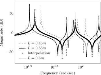
Figure2shows a clamped steel plate with given dimen-sions which is excited by a point force𝐹(𝑡)[5]. The plate is 0.2 mm thick. The system output is the displacement of the point where𝐹(𝑡)attacks. The plate length𝐿is a free variable. The model was derived in [5] using a parametric Ansys model with 225 shell elements and 1452 degrees of freedom. After evaluating it for a desired length𝐿, it can be written as port-Hamiltonian system in co-energy
repre-Figure 2: A steel plate, being excited by a force𝐹(𝑡) in normal
direction. The plate is assumed to be clamped at the edges.
sentation. We consider two plates with𝐿 = 450mm and 𝐿 = 550mm which are to be interpolated with𝜔 = 0.5. A third model has been generated for𝑥 = 500 mm and serves as reference. We chose the reduced model order 𝑞 = 12and expansion point𝑠0= 0.
Figure3shows the magnitude plots of the three di-rectly reduced systems and the interpolated system. It can be seen that the linear interpolation approximates the ref-erence system well.
Note that matrix interpolation can handle eigenvalue crossing: due to its quadratic shape, the reference sys-tem with𝐿 = 500mm has a double eigenvalue at a reso-nance frequency close to102rad/sec. In contrast, the non-quadratic plates with𝐿1= 450mm and𝐿2= 550mm both have two distinct eigenvalues at this frequency range. The interpolation method captures this behavior and approxi-mates the square plate system correctly.
Figure 3: Amplitude of test point displacement for the reduced plate
models with𝐿 = 0.45 m and 𝐿 = 0.55 m as well as the interpolated system and the reference model with𝐿 = 0.5 m.
Figure 4: Structure of the ladder network as presented in [11]. The input is the current𝐼1(𝑡), the output is the voltage 𝑈𝐶
1(𝑡) across the
first capacitor.
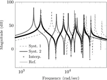
5.2 Electric Circuit Network
A ladder network is a system consisting of an arbitrary number of coupled RLC-circuits as shown in Figure 4. In [11], Matlab code for the generation of an electrical lad-der network model in standard port-Hamiltonian form is provided. The free parameters are resistance 𝑅1= 𝑅2= . . . = 𝑅, inductance𝐿1 = 𝐿2= . . . = 𝐿and capacity𝐶1= 𝐶2 = . . . = 𝐶. The input is the current𝐼1(𝑡)from an
exter-nal current source, the output is the voltage𝑈𝐶
1(𝑡)across
the first capacitor. In this example, we show a linear inter-polation of two network models in three parameters, with 𝜔 = 0.5.
System 1 has the parameters𝑅 = 0.01 𝛺,𝐿 = 1mH and𝐶 = 1 𝜇F. System 2 has the parameters𝑅 = 0.012 𝛺, 𝐿 = 3mH and𝐶 = 2 𝜇F. Both were modeled with 250 cir-cuits, resulting in𝑛 = 1000. Additionally, a reference sys-tem for linearly interpolated parameters was generated. The RK-ICOP-algorithm [12] was used to find a single ex-pansion point at 𝑠(1)0 = 33565 rad/sec for system 1 and 𝑠(2)0 = 13681rad/sec for system 2.
Figure5shows the magnitude plots of reduced (𝑞 = 10) and interpolated ladder network systems as well as the reference system with𝑅 = 0.011 𝛺𝛺,𝐿 = 2mH and𝐶 =
Figure 5: Magnitude plots of two ladder networks of order𝑛 = 1000
which differ in three parameters, their linear interpolation and a corresponding, separately reduced reference system.
1.5 𝜇F. The interpolation fits the reference system well. In fact, the new pMOR method for port-Hamiltonian systems in standard form shows good performance in interpolating three independent parameters, using models at only two sampling points in the parameter space.
6 Conclusion
This paper demonstrates that the advantages of port-Hamiltonian systems and their structure-preserving order reduction can be combined with parametric order reduc-tion. A procedure for parametric model order reduction by matrix interpolation was suggested for both co-energy representation and standard port-Hamiltonian form. The method which is to be used is determined by in which rep-resentation the system is given. For each option, there is a method which does not require the inversion of a large-scale matrix.
It was shown that an interpolation of the port-Hamiltonian system matrices has to take place in co-energy representation in order to preserve the port-Hamiltonian structure. Adjustments to the locally reduced systems were outlined, which make matrix interpolation meaningful. Both presented methods preserve the symme-try and definiteness properties, stability, and result in in-terpolated systems with identical input-output behavior. For a parametric system which is defined by a finite num-ber of sampling points, stability is obtained for all inter-adjacent, reduced systems. Simulation examples were given for both methods, for a one- and three-dimensional parameter space.
Acknowledgement: We would like to thank Dr. Jan
Mohring for making the plate model available to us.
References
1. Van der Schaft, A., “L2-Gain and Passivity Techniques in Non-linear Control”, Springer-Verlag New York, 1999.
2. Wolf, T., Lohmann, B., Eid, R., Kotyczka, P., “Passiv-ity and Structure Preserving Order Reduction of Linear Port-Hamiltonian Systems Using Krylov Subspaces”, European Journal of Control, 2010(16), 1–6. 3. Polyuga, R., et al., “Moment Matching
for Linear Port-Hamiltonian Systems”,
Proceedings of the 10th European Control Conference (ECC ’09), 2009, 4715–4720.
4. Gugercin, S., Polyuga, R., Beattie, C., Van Der Schaft, A., “Structure-Preserving Tangential Interpolation for Model Reduction of Port-Hamiltonian Systems”, Automatica, 49(9), 2012.
5. Panzer, H., Mohring, J., Eid, R., Lohmann, B., “Paramet-ric Model Order Reduction by Matrix Interpolation”, at-Automatisierungstechnik, 58(8), 2010, 475–484. 6. Polyuga, R., Van der Schaft, A., “Structure Preserving Model
Reduction of Port-Hamiltonian Systems by Moment Matching at Infinity”, Automatica, 46(4), 2010, 665–672.
7. Freund, R. W., “Krylov-subspace methods for reduced-order modeling in circuit simulation”,
Journal of Computational and Applied Mathematics, 123, 2000, 395–421.
8. Grimme, E. J., “Krylov Projection Methods for Model Reduc-tion”, PhD thesis, University of Illinois, 1997.
9. Antoulas, A. C., “Approximation of Large-Scale Dynamical Sys-tems.”, SIAM Philadelphia, 2005.
10. Eid, R., Castane-Selga, R., Panzer, H., Wolf, T., Lohmann, B., “Stability-Preserving Paramet-ric Model Reduction by Matrix Interpolation.”,
Mathematical and Computer Modelling of Dynamical Systems, 17(4), 2011.
11. Polyuga, R., “Matlab Code for Constructing the Port-Hamiltonian Representation for an n-dimensional Single-Input/Single-Output Ladder Network with Additional Resis-tors.”,http://sites.google.com/site/rostyslavpolyuga. 12. Eid, R., Panzer, H., Lohmann, B., “How to choose
a single expansion point in Krylov-based model reduction?”, Technical reports on Automatic
Control, Institute of Automatic Control, Technical University of Munich, November 2009.
Markus Giftthaler, MSc
Department of Mechanical and Process Engineering, ETH Zürich Zentrum, Sonneggstr. 3, CH-8092 Zürich, Phone: +41(0)44 63 264 80
Markus Giftthaler is with the Department of Mechanical and Process Engineering, Swiss Federal Institute of Technology, Zürich. His cur-rent research interests include parametric model order reduction by matrix interpolation, the control of thermoacoustic machines and autonomous robotic fabrication on construction sites.
Dipl.- Ing. Thomas Wolf
Institute of Automatic Control, Technische Universität München, Boltzmannstr. 15, D-85748 Garching bei München, Phone: +49-(0)89-289-15592
Dipl.- Ing. Thomas Wolf is a research assistant at the Institute of Automatic Control of the Faculty of Mechanical Engineering at the Technische Universität München. His field of research includes model order reduction of large-scale systems and port-Hamiltonian model representation.
Dipl.- Ing. Heiko K. F. Panzer
Institute of Automatic Control, Technische Universität München, Boltzmannstr. 15, D-85748 Garching bei München, Phone: +49-(0)89-289-15592
Dipl.- Ing. Heiko K. F. Panzer is a research assistant at the Institute of Automatic Control of the Faculty of Mechanical Engineering at the Technische Universität München. His research interest includes model order reduction of large-scale systems by Krylov subspace methods and parametric model order reduction by matrix interpola-tion.
Prof. Dr.- Ing. habil. Boris Lohmann
Institute of Automatic Control, Technische Universität München, Boltzmannstr. 15, D-85748 Garching bei München, Fax: +49-(0)89-289-15653
Prof. Dr.- Ing. habil. Boris Lohmann is Head of the Institute of Auto-matic Control of the Faculty of Mechanical Engineering at the Tech-nische Universität München. His research activities include model order reduction, nonlinear, robust and optimal control as well as active vibration control.