HAL Id: tel-01004370
https://tel.archives-ouvertes.fr/tel-01004370
Submitted on 11 Jun 2014HAL is a multi-disciplinary open access archive for the deposit and dissemination of sci-entific research documents, whether they are pub-lished or not. The documents may come from teaching and research institutions in France or abroad, or from public or private research centers.
L’archive ouverte pluridisciplinaire HAL, est destinée au dépôt et à la diffusion de documents scientifiques de niveau recherche, publiés ou non, émanant des établissements d’enseignement et de recherche français ou étrangers, des laboratoires publics ou privés.
The study of the oxygen controlled combustion in
downsized SI engine
Jianxi Zhou
To cite this version:
Jianxi Zhou. The study of the oxygen controlled combustion in downsized SI engine. Other. Université d’Orléans, 2013. English. �NNT : 2013ORLE2049�. �tel-01004370�
UNIVERSITE D’ORLEANS
ÉCOLE DOCTORALE SCIENCES ET TECHNOLOGIES
Laboratoire PRISME
THÈSE
présentée par :Jianxi ZHOU
Soutenue le :Pour obtenir le grade de : Docteur de l’université d’Orléans Discipline : Mécanique et Energétique
THÈSE dirigée par :
Mme Christine MOUNAÏM-ROUSSELLE Professeur, Université d’Orléans
M Fabrice FOUCHER Maitre de Conférences, Université d’Orléans RAPPORTEURS :
M. Marc BELLENOUE Professeur ENSMA Poitiers
M. Bernard LEDUC Professeur université libre de Bruxelles JURY :
M. Marc BELLENOUE Professeur, ENSMA Poitiers
M. Bernard LEDUC Professeur, Université Libre de Bruxelles M. Guillaume DAYMA Professeur, Université d’Orléans
M. Gilles CABOT Maître de Conférences, HdR, Université de Rouen M. Erwann SANSON Ingénieur de Recherche, PSA Peugeot Citroën Mme. C. MOUNAÏM-ROUSSELLE Professeur, Université d’Orléans
M. Fabrice FOUCHER Maître de Conférences, HdR, Université d’Orléans
Etude de l’effet du taux d’oxygène sur la
combustion en moteur à allumage
3
Remerciements
Cette thèse, cofinancée par la région Centre et PSA Peugeot Citroën, a été réalisée au sein de l’équipe Energie, Combustion et Moteur du laboratoire PRISME (Pluridisciplinaire de Recherche Ingénierie des Systèmes Mécanique, Energétique) de l’université d’Orléans.
Je tiens tout abord à remercier Christine Mounaïm-Rousselle, qui a dirigé cette étude, de m’avoir accueilli au sein de son équipe, de m’avoir donné l’opportunité de réaliser ce travail de thèse et de m’avoir soutenu au cours de cette thèse.
Je tiens à exprimer ma profonde reconnaissance à Fabrice Foucher, qui a codirigé cette thèse, pour son excellent encadrement, sa disponibilité, sa confiance et son soutien. Je le remercie aussi pour les agréables moments en dehors du laboratoire (Congrès, Ski …).
Je remercie Erwann Samson, ingénieur recherche du groupe PSA Peugeot Citroën, pour avoir soutenu ce projet et pour les discussions scientifiques et ses précieux conseils.
Je tiens à remercier Stéphane Richard, ingénieur recherche d’IFP Energies Nouvelles, pour les discussions et son aide sur la partie simulation LMS Amesim.
Je tiens à remercier également tous les membres de jury qui ont accepté de juger ma thèse: B. Leduc, M. Bellenoue, G. Dayma, G. Cabot, E. Sanson et tout particulièrement les deux rapporteurs, B. Leduc et M. Bellenoue pour avoir accepté d’examiner le mémoire.
Je souhaiterais ensuite exprimer tout ma reconnaissance pour tous les membres des équipes techniques et administratives du laboratoire pour leur aide précieuse à ce travail : Sylvie Plessard, Nicolas Dumuis, Yahia Haidous, Benoit Bellicaud, Benoit Clavier et Pierre. Je souhaiterais exprimer ma grand merci à Bruno Moreau et Julien Lemaire, avec qui j’ai appris sur la conception et la mise en place des dispositifs expérimentaux, surtout, durant les moments difficiles, moteur cassé, problème de baies d’analyse de gaz ...
Je voudrais aussi dire mon profond merci à tous les amis et collègues: Jérémie, Toni, les deux excellents amis et collègues dans le même bureau au début de ma thèse, grâce à eux, je me suis initié aux connaissances du moteur. Guillaume, J-B, Pierre, Padipan, Antonio, Shadi, Benedicte, Etienne, Mathieu, les amis et collègues dans même bureau de ‘open space’. Je tiens aussi à exprimer mon merci à tous les amis dans le labo PRISME : Christophe, Chao, Jamil, Haïfa, Yan-Aël, Amine, Audrey, Arnaud, comme compagnons de tous les jours, pour les discussions, les cafés, les soirées et les autres sorties.
Je souhaiterais aussi encore remercier à les amis dans le labo Coria (où j’ai fait deux stages), François-Xavier, mon encadrant, qui m’appris les outils numériques et notion de programmations. François, Guillaume, Jieshen, Jérémie, Arnaud, Bruno, pour les discussions et les soirées poker et foot.
Je voudrais finir par remercier toute ma famille, tout particulièrement mes parents qui m’ont permis de poursuivre mes études par leur soutien moral et financier. Et ma femme Suli, merci pour les soutiens des moments difficiles, et merci pour m’avoir donné le plus beau cadeau, mon fils.
5
Table of contents
Introduction générale ... 17
1
Chapter 1 General study of bibliography ... 23
1.1 Actual emission problems and fuel economy ...24
1.2 Introduction to SI engine and its new technologies ...25
1.3 Normal Combustion in SI engine ...28
1.3.1 Laminar premixed combustion ...28
1.3.2 Turbulent premixed combustion ...31
1.4 Abnormal combustion ...35
1.4.1 Pre-ignition ...36
1.4.2 Engine knock ...36
1.5 Application of Oxygen-Controlled combustion in downsized SI engine ...38
2
Study of oxygen controlled combustion in engine ... 45
2.1 Introduction ...45
2.2 Experimental setup ...45
2.2.1 Engine characteristics ...45
2.2.2 Engine control and measurement ...47
2.3 Combustion analysis ...47
2.3.1 Single zone analysis model ...47
2.4 Emission analysis ...49
2.4.1 Converting humid gas type to dry gas type ...49
2.4.2 Equivalence ratio of 5 gases ...50
2.5 Operating conditions and engine parameters ...52
2.6 Results and discussion ...55
2.6.1 Indicated mean effective pressure ...55
2.6.2 HC emissions ...58 2.6.3 NOx emissions ...60 2.6.4 CO emissions ...62 2.6.5 CO2 emissions ...64 2.6.6 Combustion characteristics ...66 2.7 Conclusions ...67
6
3
Characteristics parameters of combustion for oxygen-controlled fuel
mixture ... 71
3.1.1 Laminar burning velocity ...71
3.1.2 Correlations of laminar burning velocity ...75
3.2 Experimental set-up ...78
3.3 Methodology to analyze flame propagation ...80
3.3.1 Laminar burning velocity determination ...80
3.3.2 Markstein Length ...82
3.4 Validation of the methodologies: case of iso-octane/air mixture. ...83
3.5 Results and discussion ...84
3.5.1 Effect of oxygen enrichment ...84
3.5.2 Effect of CO2 addition ...85
3.5.3 Effect of O2 and CO2 on adiabatic flame temperature ...86
3.5.4 Markstein lengths ...87
3.5.5 Experimental correlation for laminar burning velocity ...89
3.6 Conclusions ...89
3.7 Data avalaible : ...90
3.8 Auto-ignition delay of Isooctane/O2/N2/CO2 mixtures ...91
3.9 Conclusions ...94
4
Combustion modeling ... 97
4.1 Introduction ...97
4.2 Combustion modeling using Amesim ...98
4.2.1 Energy conservation equations ...98
4.2.2 Combustion heat release ...99
4.2.3 Tabulation of the mean flame surface ...100
4.2.4 Flame wrinkling ...101
4.2.5 Knock modeling ...101
4.2.6 Knock intensity estimation ...103
4.3 Adaptation of Amesim model for oxygen controlling engine ...104
4.3.1 Laminar flame speed correlation ...105
4.4 Calibration process ...106
4.5 Amesim model results ...108
4.5.1 Validation of pure compression cycle ...108
7
4.5.3 Calibration of in-cylinder pressure ...111
4.5.4 Combustion characteristics ...118
Effect of O2 percentage on combustion characteristics ...118
Effect of equivalence ratio on combustion characteristics ...123
Effect of IMEP on combustion characteristics ...125
Parametric study of combustion characteristics ...127
4.5.5 Knock estimation and sensitivities ...132
4.6 Conclusions ...138
5
Conclusions and perspectives ... 141
Conclusions et perspectives (version français) ... 144
6
ANNEXES ... 154
Engine efficiencies and energy losses ...156
9
List of figures
Figure 1-1. Evolution of mean CO2 emission value for new cars in Europe ...25
Figure 1-2 the structure of a SI engine with turbo-compressor ...26
Figure 1-3 diagrams for illustrating engine efficiency ...26
Figure 1-4. mechanism of a laminar premixed combustion ...29
Figure 1-5. Structure of a laminar premixed combustion ...29
Figure 1-6. the structure of energy cascade (Bougrine 2012) ...31
Figure 1-7. Peters-Borghi Diagram of combustion regime (Borghi et al. 1984) ...34
Figure 1-8. Cylinder pressure curves for normal and abnormal combustion (Winklhofer 2009) ...35
Figure 1-9. Time-series of high speed direct combustion images with the H2-O2-Ar mixture (equivalence ration=1.0, P0=40kPa, T0=323K,
θ
i = 355 deg and knock intensity KI = 1.173Mpa)(Kawahara 2009) ...37Figure 1-10. Comparison of current EGR dilution system (left), oxygen controlled by membranes (middle) and oxygen controlled with CO2 dilution (right). ...39
Figure 1-11. effects of equivalence ratio on CSI, i ,IMEP (left) and CO, HC, NOx emissions (right) ...40
Figure 2-1. Scheme of EP6 mono-cylinder engine ...46
Figure 2-2. Real Image of engine ...46
Figure 2-3. Equivalence between N2 dilution (O2 < 20.9%) or O2 enrichment (O2 > 20.9%) and EGR percentage for a fixed equivalence ratio ...54
Figure 2-4. Presentation of the different operation points employed in engine test bench ...55
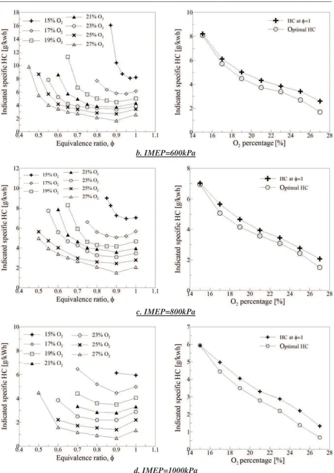
Figure 2-5. the evolution of indicated specific fuel consummation (SFC) versus equivalence ratio with different IMEP (a. IMEP=400kPa, b. IMEP=600kPa, c. IMEP=800kPa, d. IMEP=1000kPa) ...57
Figure 2-6. the evolution of indicated specific HC emissions versus equivalence ratio with different IMEP (a. IMEP=400kPa, b. IMEP=600kPa, c. IMEP=800kPa, d. IMEP=1000kPa)59 Figure 2-7. the evolution of indicated specific NOx emissions versus equivalence ratio with different IMEP (a. IMEP=400kPa, b. IMEP=600kPa, c. IMEP=800kPa, d. IMEP=1000kPa)61 Figure 2-8. Evolutions of the indicated specific NOx emission versus O2 percentage with different Indicated mean pressure at stoichiometry ...62
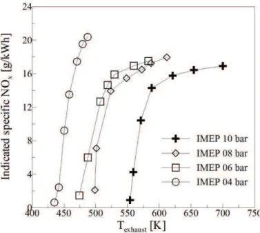
Figure 2-9. Evolutions of the indicated specific NOx emission versus exhaust temperature with different Indicated mean pressure at stoichiometry ...62
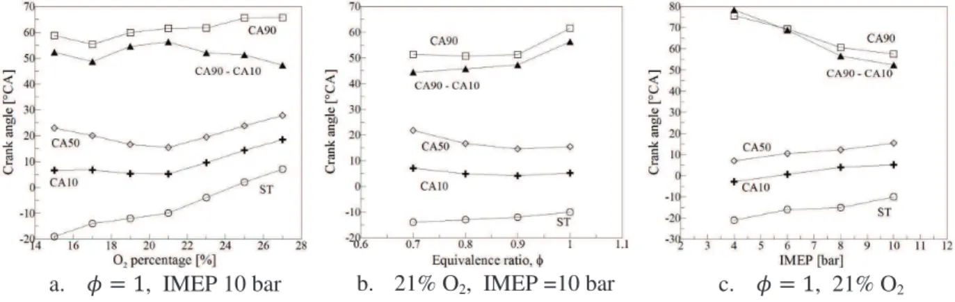
Figure 2-10. the evolution of indicated specific CO emissions versus equivalence ratio with different IMEP (a. IMEP=400kPa, b. IMEP=600kPa, c. IMEP=800kPa, d. IMEP=1000kPa)64 Figure 2-11. the evolution of indicated specific CO2 emissions versus equivalence ratio with different IMEP (a. IMEP=400kPa, b. IMEP=600kPa, c. IMEP=800kPa, d. IMEP=1000kPa)66 Figure 2-12. combustion characteristics for three different cases( a. , IMEP 10 bar, b. 21% O2, IMEP =10 bar, c. , 21% O2) ...67
Figure 3-1. description of the structure of spherically expanding laminar flame front ...72
10
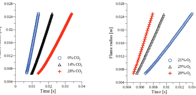
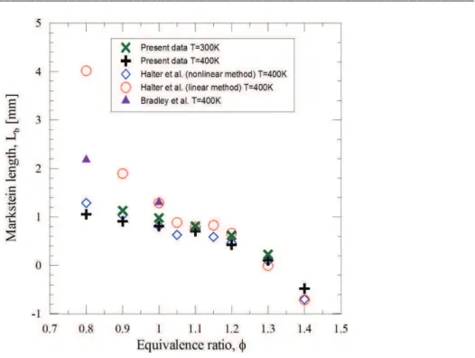
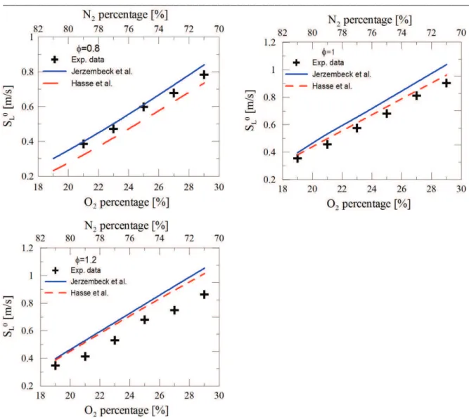
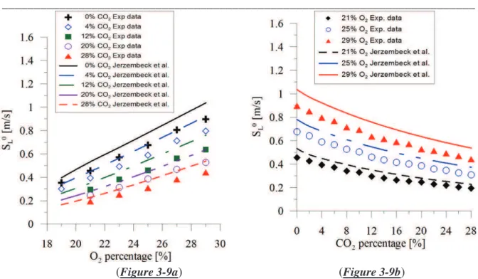
Figure 3-3. Example of the flame front at 9ms, 15ms and 21ms after start of ignition. ...80 Figure 3-4. Flame radius as a function of time for different experimental condition ...81 Figure 3-5. Unstretched propagation flame speed determination for different experimental conditions. Square symbol: experimental velocity as function of flame stretch. Continuous lines: linear methodology. Dashed line: nonlinear methodology. ...82 Figure 3-6. Experimental laminar burning velocities of isooctane-air mixture at two initial temperatures (300 K and 400 K).Comparation with previous studies in the literature(Davis et al. 1998) (Huang et al. 2004) (Freeh et al. 2004; Kumar et al. 2007) (Bradley et al. 1998; Halter et al. 2010). ...83 Figure 3-7. Markstein length versus the equivalence ratio for isooctane mixture. Comparison with previous studies (Bradley et al. 1998; Halter et al. 2010). ...84 Figure 3-8. Laminar burning velocities as function of the amount of oxygen in air-isooctane mixture for 3 equivalence ratios (Tini = 373 K, Pini = 1 atm). ...85 Figure 3-9. Laminar burning velocities versus O2 and CO2 percentage at stoichiometric equivalence ratio (Tini = 373 K, Pini = 1 atm). ...86 Figure 3-10. Simulated adiabatic flame temperature versus O2 (7a) and CO2 (7b) percentage at stoichiometric equivalence ratio (Tini = 373 K, Pini = 1 atm). ...87 Figure 3-11. Laminar flame velocity as a function of the adiabatic temperature ...87 Figure 3-12. Markstein length evolution versus O2 (a) and CO2 (b) percentage for 3 different cases (Tini = 373 K, Pini = 1 atm) ...88 Figure 3-13. Comparison between estimated values (dotted lines) and experimental data for various CO2 and O2 percentages. ...89 Figure 3-14. Ignition delays versus O2 and CO2 percentage for stoichiometric
iso-octane/O2/N2/CO2 mixture with 1000/T=1.5 (1/K), P=20 bar. Comparison between simulation data and correlation results. ...92 Figure 3-15. Ignition delays versus pressure for iso-octane/O2/CO2/N2 mixture (with 20% CO2, 21% O2 and T = 666 K) ...93 Figure 3-16. Ignition delays versus temperature for iso-octane/O2/CO2/N2 mixture (with 20% CO2, 21% O2 and P=60 bar) ...93 Figure 4-1. Evolution of mean flame surface –based on real configuration ...100 Figure 4-2. Example of knock crank angle with spark advance before and after top dead center (red line: an example of in-cylinder pressure at 10 bar IMEP and 27%O2, black line: supposed pressure) ...104 Figure 4-3. Amesim model for oxygen controlling engine ...105 Figure 4-4. illustration of simulation process ...107 Figure 4-5. Validation of pure compression process. From bottom to up, the intake pressures are from 6 bars to 16 bars with the steps of 2 bars ...109 Figure 4-6. Presentation of the different operation points employed in engine test bench and the Amesim combustion model calibration process (1400 rpm). ...109 Figure 4-7. Intake pressure(a) and spark advance (b) versus equivalence ratio for different cases of O2 percentages ...111 Figure 4-8. Fuel mass flow rate versus equivalence ratio for different cases of O2 percentages
11
Figure 4-9. Comparison between experimental and simulated cylinder pressure curve for different engine load at 1400 rpm. ...113 Figure 4-10. Comparison between experimental and simulated cylinder pressure curve for different equivalence ratio at 1400 rpm. ...113 Figure 4-11. Relative error of IMEP (a) and maximum in-cylinder pressure (b) as function of IMEP. ...114 Figure 4-12. Relative error of IMEP (a) and maximum in-cylinder pressure (b) as function of equivalence ratio. ...114 Figure 4-13. Relative error of IMEP (a) and maximum in-cylinder pressure (b) as function of O2 precentage. ...115 Figure 4-14. integral length scales and tumble values obtained by optimizing the in-cylinder pressure. ...116 Figure 4-15. integral length scales and tumble values obtained by optimizing the in-cylinder pressure at IMEP=10 bar. ...116 Figure 4-16. integral length scales and tumble values obtained by optimizing the in-cylinder pressure at unit equivalence ratio. ...117 Figure 4-17. integral length scales (a) and tumble values (b) versus intake pressure for IMEP at 10 bar. ...118 Figure 4-18. Evolution of the mean in-cylinder pressure at stoichiometric and IMEP=1000kPa
...119
Figure 4-19. Laminar burning velocity versus crank angle degree with different O2 percentages at stoichiometric and IMEP=1000kPa ...119 Figure 4-20. Flame surface (a) and flame wrinkling (b) versus Crank angle with different O2 percentages at unit equivalence ratio and IMEP=1000kPa ...120 Figure 4-21. Evolution of turbulent flame velocity with different O2 percentages at
stoichiometric equivalence ratio and IMEP=1000kPa ...121 Figure 4-22. Ratio of the characteristic length and velocity scales versus crank angle degree for different O2 percentages. ...121 Figure 4-23. Ratio of the characteristic length and velocity scales versus O2 percentage for two crank angle degree cases ...122 Figure 4-24. Comparison of the combustion traces in the Peters-Borghi diagram for different O2 percentages ...123 Figure 4-25. Operating conditions for combustion analysis ...124 Figure 4-26. Ratio of the characteristic length and velocity scales versus crank angle degree for different equivalence ratios. ...124 Figure 4-27. Ratio of the characteristic length and velocity scales versus equivalence ratio for two crank angle degree cases ...124 Figure 4-28. Comparison of the combustion traces in the Peters-Borghi diagram for different equivalence ratios at IMEP=10 bar ...125 Figure 4-29. Operating conditions of different IMEP for combustion analysis ...125 Figure 4-30. Ratio of the characteristic length and velocity scales versus crank angle degree for different IMEP. ...126 Figure 4-31. Ratio of the characteristic length and velocity scales versus IMEP for two crank angle degree cases ...126
12
Figure 4-32. Comparison of the combustion traces in the Peters-Borghi diagram for different equivalence ratios ...127 Figure 4-33. Evolution of in-cylinder pressure varying laminar flame speed with two different cases of equivalence ratio at IMEP=10bar ...128 Figure 4-34. evolution of in-cylinder pressure varying spark ignition advance for three
different cases of O2 percentage at IMEP=10bar and stoichiometric equivalence ratio (X=1, 2, 3). ...130 Figure 4-35. Evolution of in-cylinder pressure varying the intake temperature for three
different cases of O2 percentage at IMEP=10bar and stoichiometric equivalence ratio (X=1, 2, 3) ...131 Figure 4-36. Laminar burning velocity versus crank angle for two different cases. Left:
variation of spark advance, Right: variation of intake temperature ...132 Figure 4-37. Behavior of spark advance (left) and intake temperature (right) in Peters-Borghi diagram. ...132 Figure 4-38. Examples of absolute (left hand) and high-passed filtered with 4 kHz cut-off frequency (right hand) cylinder pressure traces at IMEP 10 bar and . ...134 Figure 4-39. High-passed filtered cylinder pressure traces for 100 consecutive cycles at IMEP 10 bar and . ...135 Figure 4-40. Absolute values of experimental indicators (left) and normalized MAPO, IMPO, simulated KI (right) versus O2 percentage ...136 Figure 4-41. Evolution of knock intensity (KI) by varying laminar flame speed and
auto-ignition delay ...137 Figure 4-42. Evolution of knock intensity (KI) by varying spark advance with adv= Advref +
∆
CA ...138 Figure 4-43. Evolution of knock intensity (KI) by varying intake temperature with Tintake= Tintake,ref +∆
Tintake ...138 Figure 6-1. An example of Clapeyron diagram with operating conditions as: engine speed 1400 rpm, Pintake = 0.6 bar, Spark advance = 21 CAD ...15513
List of tables
Table 1-1. European anti-pollution standards (in g/km) for gasoline engine cars
(http://en.wikipedia.org/wiki/European_emission_standards). ... 24
Table 1-2. Engine parameters influencing knock tendency.(Ferguson 1986) ... 38
Table 2-1. determination of the volume fraction of air, O2 and N2 for different cases. ... 52
Table 2-2. Equivalence between N2 dilution (O2 < 20.9%) or O2 enrichment (O2 > 20.9%) and EGR percentage for a fixed equivalence ratio. ... 54
Table 3-1. values of the constants for different dilution at stoichiometric condition. ... 78
Table 3-2. values of the constants and for different equivalence ratios. ... 78
Table 3-3. A summary of various experimental conditions for isooctane ignition delay test (Scott 2009) ... 91
Table 4-1. Correlation parameters in laminar flame speed correlation. ... 106
Table 4-2. Operation conditions of engine bench tests at 10 IMEP ... 110
14
Nomenclature
Latins Symboleslaminar flame surface turbulent flame surface
c progress variable of combustion -
C constant coefficient -
CAxx Crank angle degree when xx% of fresh air/fuel mixture is burned
CAD
Cp specific heat coefficient at constant pressure -
Cv specific heat coefficient at constant volume -
Da Damköhler number -
heat diffusivity of fresh gases
energy spectrum J
h mass enthalpy J/kg
turbulent kinetic energy
K total stretch rate 1/s
Ka Karlovitz number -
size of eddies m
! burned gas Markstein length m
Le Lewis numbers -
"# Lewis numbers of the deficient -
"$ Lewis numbers of the excess -
turbulent integral length scale m
m Mass kg
% constant coefficient -
&'() engine rotation speed *+
pressure pa
PCI heating value of fuel J/kg
,- turbulent intensity m/s
./ heat produced by combustion J
.0 wall heat loss J
r Flame rayon m
1" Reynolds number -
2/ Schmidt number -
2 laminar flame speed m/s
23 mean flame surface
2 turbulent flame surface
t time s
T temperature K
/ chemical time scales s
characteristic time of turbulent s
4-, 5-, 6- velocity fluctuations m/s
7 volume, volume fraction 8
7( stretched propagation flame velocity m/s
7(9 unstretched propagation flame velocity m/s
W work applies to piston, molecular weight J
15
x, y, z spatial coordinate m
: mass fraction -
Grecs Symboles
constant coefficient -
Crank angle degree CAD
; Flame thickness, characteristic thermal thickness m
< isentropic coefficient -
= equivalence ratio -
∆ variation -
> / Crank angle duration of combustion CAD
>?@ Crank angle duration of initial flame development CAD
>?A half crank angle degree of the combustion CAD
B Zeldovich number, constant coefficient -
C density DE 8
F fresh gases heat conductivity G H
I flame wrinkling factor -
5 kinematic viscosity
JK Kolmogorov length scale m
J/L3! combustion efficiency -
M dissipation rate E 8
NO'P residual gas mass fraction -
Q the expansion factor -
RS stoichiometric coefficient of species i -
T efficiency function of the turbulent flow on the flame strain - Indice b burned gases c chemical, combustion UV cylinder UW* carburant "XX effective XD Fresh gases i inflammation L laminar t turbulent u unburned gases Abbreviations 0D zero-dimensional
16 ATDC after top dead center
BTDC before top dead center
BMF burned mass fraction
CAD crank-angle degree
CAXX crank angle degree for which XX% of the cumulative heat release is released
CO carbon monoxide
CO2 carbon dioxide
CoV coefficient of variation
CFD Computational Fluid Dynamics
EGR Exhaust Gaz Recirculation
HCCI Homogeneous Charge Compression Ignition
IC internal combustion
IMEP indicated mean effective pressure
KI knock intensity
LES Large Eddy Simulation
LIF Laser Induced Fluorescence
MN methane number
N2 nitrogen
NOx nitrogen oxide
O2 oxygen
OST optimum spark timing
RON research octane number
RPM Round per minute
SFC Specific fuel consumption
SI spark ignition
ST spark timing
TDC top dead center
Introduction générale __________________________________________________________________________
19
Le moteur à combustion interne, que ce soit à allumage par étincelle ou par compression, a su s’imposer comme source motrice pour la plupart des véhicules de transports et notamment des automobiles. Ce système a donc pu profiter de nombreux développements depuis plus d’un siècle permettant d’atteindre des performances exceptionnelles en termes de rendement énergétique et d’émissions polluantes. Malgré ces améliorations constantes, le transport, dû à l’utilisation des moteurs à combustion interne, est l’une des sources majeures d’émissions de gaz à effets de serre et d’autres émissions polluantes nocives pour notre planète et notre santé. Parallèlement à l’enjeu de réduction des émissions polluantes, la diminution certaine et relativement proche de nos ressources mondiales pétrolières nécessite de trouver de nouveaux procédés de motorisation et/ou de modes de combustion afin de réduire la consommation en carburant des moteurs à combustion interne, challenge qu’essayent de tenir les constructeurs automobiles et les organismes de recherche. L’objectif scientifique de l’équipe Energétique, Combustion et Moteurs du laboratoire PRISME est en parfaite symbiose avec ce challenge soit en apportant des éléments nouveaux sur les phénomènes mis en jeu, soit en proposant des nouveaux systèmes de motorisations ou encore en optimisant le contrôle-moteur, maillon final d’optimisation du groupe moto-propulseur.
Actuellement, l’une des voies potentiellement envisagées pour augmenter le rendement, et donc par là-même diminuer la consommation en carburant, est de suralimenter massivement les moteurs. Ainsi, tout en maintenant constante la puissance, l’augmentation du rendement est obtenue par la conjoncture de deux effets : un remplissage optimum de la chambre de combustion grâce à l’utilisation d’un turbocompresseur permettant de suralimenter l’admission et la diminution des frottements mécaniques résultant de la diminution de la taille et de la masse des pièces mécaniques en mouvement. Ainsi, grâce à ce concept, dénommé «Downsizing», les gains de rendement peuvent atteindre jusqu’à 20%.
Malgré la simplicité apparente de ce concept, de nombreuses questions liées au déroulement de cette combustion restent en suspens. En effet, la combustion se déroule dans des plages de pression et de température beaucoup plus importantes que dans un moteur conventionnel ; de plus, ce mode de combustion est très souvent associé à une dilution massive des gaz frais par l’utilisation de l’EGR (Exhaust Gas Recirculation). Expérimentalement, il a été observé que la conjoncture de ces deux points pouvait générer des combustions anormales pouvant mener à la destruction du moteur, ou inversement des combustions dégradées et incomplètes.
L’objectif de cette thèse est donc d’étudier la combustion in-situ dans le cas de fonctionnement d’un moteur à allumage commandé suralimenté mais en contrôlant le taux d’oxygène afin d’en étudier son effet. Peu d’études expérimentales et numériques existent à ce jour permettant de prédire le développement de la combustion dans ces conditions si particulières.
Le premier chapitre de ce mémoire est consacré à l’étude bibliographique de manière générale sur le fonctionnement du moteur allumage commandé et plus particulièrement dans des conditions de suralimentation. Une attention particulière est portée sur les deux paramètres importants pour les conditions de cliquetis : la vitesse de combustion laminaire et le délai d’auto-inflammation.
Le deuxième chapitre est consacré à la description du dispositif expérimental et des méthodes d'analyse numérique pour le traitement des résultats. Les résultats expérimentaux obtenus sur banc moteur monocylindre en variant le taux d’oxygène à l’admission y sont présentés et analysés.
Introduction générale __________________________________________________________________________
20
Le troisième chapitre expose l’étude réalisée pour estimer les paramètres caractéristiques de la combustion. Dans ce chapitre, l'enrichissement de l’oxygène sur la combustion laminaire de l’iso-octane avec l'oxygène dans des conditions proches des Conditions moteurs y est discuté. Des comparaisons des mesures de vitesse de combustion laminaire avec les données issues d’une simulation avec le logiciel Cantera appliquée avec deux schémas chimiques y sont discutées. Les données concernant la longueur Markstein y sont également présentées. Un mélange enrichi en oxygène semble être très intéressant pour augmenter la vitesse de combustion laminaire et la stabilité de la flamme. Le délai d'auto-inflammation a aussi été déterminé pour les mélanges d’Isooctane/O2/N2/CO2, en utilisant l'outil Senkin. Ensuite, pour obtenir une correction plus précise pour le cas de la simulation AMESIM, les conditions initiales des mélanges Isooctane/O2/N2 ont été définies en tenant compte des données
calculées et expérimentales de pression et de température.
Le quatrième chapitre est dédié à la présentation du logiciel commercial AMESim, au développement nécessaire pour simuler les variations des taux d’oxygène à l’admission en particulier les paramètres tels que la vitesse de combustion laminaire et le délai d’auto-inflammation. La prédiction de l’évolution de la vitesse de combustion turbulente dans le cylindre durant le cycle a permis ainsi de classifier la combustion dans un diagramme de combustion turbulente (type Peters-Borghi) et d’estimer l’intensité du Cliquetis et sa sensibilité avec différents paramètres.
En conclusion, les résultats principaux sont synthétisés pour dégager les principales analyses faites sur les modes de combustion essence à taux d’oxygène contrôlé, et pour proposer des perspectives d’études.
Chapter one
__________________________________________________________________________
1. General study of bibliography __________________________________________________________________________
1. General study of bibliography __________________________________________________________________________
23
1 Chapter 1 General study of bibliography
Considering lack of oil storage and stringent legislation on emission, improving the engine efficiency in combination with a decrease of air pollution becomes a significant challenge for engine manufacturers. For Spark-Ignition (SI) engine, one of the potential solutions is to shift towards ‘downsizing’ engine. In order to maintain the engine power output, boosting technologies, either supercharging or turbo-charging, are generally employed because they allow more air to be pumped into the engine and therefore increase the engine power density. In this thesis, engine combustion with controlling oxygen concentration in air is discussed. In one hand, for oxygen-enriched combustion, engine power density can be improved with same intake pressure level. Thus, oxygen-enriched combustion can be used either as a kind of boosting way for increasing engine output or as a combustion enhancer when engine works in low load or cold start. Several studies performed with oxygen enrichment in SI engines showed positive effects: Reduction in Unburned Hydrocarbon fuel (UHC) and CO (Kajitani et al. 1993; Ng et al. 1993; POOLA et al. 1995; Poola et al. 1996), Optimization of downsizing due to the direct effect on the combustion process and overall engine thermodynamics(Caton 2005), Increase in flame propagation velocity (Quader 1978; Kajitani et al. 1992; Poola et al. 1998) and so on. In the other hand, low oxygen concentration in air (or N2 dilution) can be considered as an alternative to exhaust gas recirculation (EGR) which is widely investigated in recent years (Van Blarigan et al. 2012; Mounaïm-Rousselle et al. 2013).
Moreover, controlling oxygen concentration in air can be done by selective permeation through a non-porous polymeric membrane, air can be recomposed with oxygen enrichment or nitrogen dilution for engine applications (Koros et al. 1987).this kind of polymeric membrane technology is now extensively researched and applied (Poola et al. 1998; Coombe et al. 2007; Favre et al. 2009).
Thus, the first purpose of this thesis is to investigate the impact of oxygen concentration controlled on engine performance and emissions using bench tests, and give a global overview of optimized engine operation points with lowest SFC and exhaust gas emissions. In order to study more details of engine combustion with oxygen controlling, containing turbulent flame velocity in engine, flame wrinkling, knock prediction and so on, the Amesim commercial software, with the combustion model developed by IFP-EN was employed. Compare to the other two zone models, Amesim combustion provides the following advantages: firstly, Amesim enables us to address the various physical domains involved in vehicle and engine system simulation with a high level of details (IFP-engine library, 2008). Thanks to this advantage, Amesim model can be set up with reference to the experimental configuration, for example, intake and exhaust tube, engine valves, turbo-compressors and so on. Secondly, the combustion model proposed and developed by IFP-EN gives an accurate description of physical processes. Although this combustion model is based on weak assumption for the mean flame geometry, the employment of the flame surface, turbulent intensity, and laminar and turbulent flame speed gives a realistic physical signification for the in-cylinder combustion process.
Thus, this chapter is dedicated to
Firstly discuss about actual emission problems and fuel economy give a brief introduction of SI engine and new technologies
1. General study of bibliography __________________________________________________________________________
24 study the normal combustion in SI engine study the abnormal combustion in SI engine
investigate the Oxygen-Controlled combustion in engine
1.1 Actual emission problems and fuel economy
Nowadays, vehicle exhaust gas emissions become a serious problem with shapely increasing of car numbers. In present, the main pollutant emission refers to CO, HC, NOx, and PM (particulate matter). Carbon monoxide, produced mainly by incomplete combustion, can reduce the oxygen percentage in the bloodstream and is particularly dangerous for people with heart disease. Hydrocarbon is mainly due to incomplete or no combustion of fuel. It can form ground-level ozone with the presence of nitrogen oxides. Moreover, it is also toxic, with the potential to cause cancer. Nitrogen oxide is the main factor of ozone formation. The well known principal mechanism of Nitrogen oxide formation is the Zeldovich one, which depends on high temperature condition which could be inside engine. Particulate matter which is smaller than order of 10 micrometers can penetrate the deepest part of lung and cause health problem.
Since the first pollutant standard in 1972, the restriction has become more and more stringent. European pollutant standards (in g/km) for gasoline engine cars are exhibited in Table 1-1. From 1992 to now, the norm of CO is reduced about three times and the norm of HC+NOx is
reduced more than six times. In Euro 3, HC and NOx are considered separately. From Euro 5,
NMHC (non-methane hydrocarbons) is also separately counted from THC (total hydrocarbon) and PM emission is regulated for the first time.
standard date CO THC NMHC NOx HC+NOx PM
Euro 1 07/1992 2,72 - - - 0,97 - Euro 2 01/1996 2,2 - - - 0,5 - Euro 3 01/2000 2,3 0,2 - 0,15 - - Euro 4 01/2005 1,0 0,1 - 0,08 - - Euro 5 09/2009 1,0 0,1 0,068 0,06 - 0,005 Euro 6 09/2014 1,0 0,1 0,068 0,06 - 0,005
Table 1-1. European anti-pollution standards (in g/km) for gasoline engine cars (http://en.wikipedia.org/wiki/European_emission_standards).
Meanwhile, Carbon dioxide (CO2), a normal combustion product, which can trap the earth’s
heat and thus produces the green house effect. The European Union has set itself the target of reducing emissions by 20% global CO2 emissions between 1990 and 2020. For automobile
sector, an average reduction of 40% of the CO2 emissions of new vehicles is required between
2007 and 2020. In Figure 1-1, the evolution of mean CO2 emission value for new cars in
Europe is described. France and Portugal are both countries which reached 140 g/km of CO2
emission value in 2008. However, many efforts should be done for the next several years. The European objective of 2015 and 2020 are respectively 130g CO2/km and 95g CO2/km for
average vehicle emissions, which is far away from general European trend as showed in Figure 1-1. As CO2 is one of the main products of combustion, the best way to meet the
1. General study of bibliography __________________________________________________________________________
25
Figure 1-1. Evolution of mean CO2 emission value for new cars in Europe (Source CCFA http://www.developpement-durable.gouv.fr/IMG/pdf/ccfa.pdf)
Therefore, facing to these environmental and human health problems, it is necessary to optimize the engine operation to minimize pollutant emissions while providing better engine performance and less fuel consumption. Following these strategic clues, in car manufacture, vehicle engine is studied in details using both experimental and numerical methods, and new technologies are well developed for new engine generation.
1.2 Introduction to SI engine and its new technologies
In SI engine, the power is produced by the combustion of an air/fuel mixture inside a cylinder, in which the piston moves in a reciprocating motion. Figure 1-2 describes the structure of a SI engine with turbo-compressor. The engine is supplied with an air/fuel mixture, obtained by intake port injection or direct injection inside the cylinder. The amount of admitted air is controlled by a valve located in the intake pipe. One of main factor for engine power release is the quantity of introduced air/fuel mixture. Engine load is normally characterized by air filling in cylinder, which is the ratio between real air mass presented in cylinder and ideal air mass could be contained in cylinder under standard conditions (i.e. atmosphere pressure, 20 °C). Inside the cylinder, the air and vaporized fuel are transformed into a gas mixture. Ignition can then be triggered by an electrical spark, causing a local rise of temperature, initialing radicals’ formation, and then a flame front propagating in the chamber.
Recently, more and more vehicles are equipped with Turbo-compressor in order to improve the power output with same engine capacity. As showed in Figure 1-2, exhaust gas is used to drive the Turbine, while the waste-gate controls the functionality of turbine. By the mechanical connection between turbine and compressor, compressor is driven to compress the ambient air into the intake tube with higher boosted pressure (Pboost).
________________________
Figure 1-2 the
In order to meet regulation sta The first way is to reduce th temperature and pressure of ad other way is the pollution pos normally used to minimize the solve nearly 100% of the po combustion control (CITEPA combustion control is still nece Apart from pollutants emissio engine efficiency while impr reduction of CO2 emission. E
perform useful work to the tot
1-3, the energy efficiency of an
Figure 1-3
1. General study ______________________________________
26
e structure of a SI engine with turbo-compres
standards, two ways can be employed practical the pollution emission by combustion contr admission gas mixture, the EGR rate, spark tim
ost-treatment. For gasoline engine, three-way the pollutants emission. Although the pollution pollution, the relative cost is much higher (2 PA 2010) . Thus, investigation of pollutan ecessary to meet future emission regulation.
ions, another major challenge for car manufac proving fuel economy, which is also the ma Engine efficiency is the ratio of the amount otal energy contained in the fuel .As described
an internal combustion (IC) engine depends m
3 diagrams for illustrating engine efficiency
y of bibliography ________________
ressor
cally(CITEPA 2010). trol (ex. control the timing and etc). The y catalytic (TWC) is on post-treatment can (2 to 5 times) than ants emission using actures is to increase ain strategy for the nt of energy used to ed in diagram Figure mainly on:
1. General study of bibliography __________________________________________________________________________
27
• Its compression ratio and the isentropic coefficient of gases mixture, which are the two parameters determining theoretical thermal efficiency.
• Heat loss during the compression and expansion phases
• Pumping losses of the gas stream during the intake and exhaust stroke. • Energy loss by exhaust gases and blow-by
• Losses due to non-instantaneous combustion and cycle variation • Mechanical losses due to friction
• Energy used for training of auxiliaries
In order to increase the engine efficiency as well as reduce pollutants emission, several new technologies are invented for SI engine in recent years. These new technologies are either changing engine architectures or using new concept of air/fuel mixture. The former catalog can be globally summarized as:
Gasoline Direct Injection (GDI): The fuel is injected directly into the chamber by high pressure injectors (100 to 200 bars). The idea of GDI is to reduce the consumption by decreasing pumping losses due to gas transfer. Moreover, the spray evaporation cools the fuel-air mixture down, which may push back knock occurrence and therefore enable the use of higher volumetric compression ratios to improve the engine efficiency. Compare to port fuel injection, GDI has also the advantage of allowing a precise control of the fuel quantity injected in each cylinder. A major challenge of such a technology is to obtain a homogeneous air-fuel mixing and to avoid interactions between the spray and the engine walls.
Downsizing concept: The engine volume is reduced and the engine volumetric efficiency is improved by combining two key technologies: direct injection and turbo-charging. As the engine size is reduced, wall heat loss and friction can therefore be decreased. Generally, direct injection can not only decrease the in-cylinder temperature, that may prevent knock occurrence, but also give a better control of the injected fuel quantity as function of the trapped air quantity. Moreover, turbo-charging decreases pumping losses and improves exhaust gas scavenging which consequently allows a reduction of knock occurrence at high loads. Finally, higher high-pressure loops can be normally obtained in downsized engines which may lead to a better engine efficiency.
Variable Valve Timing (VVT): It allows the lift, duration or timing of intake and/or exhaust valve to be changed via the Engine Control Unit (ECU) during engine operation. VVT approaches are generally performed by adjusting geometrically the camshaft phasing. Normally the valve timing is well set for adapting different phases of engine operation mode: at idle phase, the inlet camshaft opens late and consequently, closes late as well, and the exhaust camshaft is set much before Top Dead Center (TDC). So that the air filing is minimized, this leads to smooth idling. At power phase, the exhaust valves are open late to maintain the expansion of burned gases pushing against the piston longer. Meanwhile the inlet valves open after TDC and close well after BDC to let the dynamic self-charging effect of the entering air increase power. At torque phase, Inlet valves need open early, so it close early as well, which avoids pressing out the fresh gases to achieve maximum torque. And the exhaust camshafts close just before TDC, to avoid the residual gases trapped in the cylinder.
1. General study of bibliography __________________________________________________________________________
28
The other new technologies of this catalog are also widely discussed and researched such as Variable Compression Ratio (VCR), Hybrid electric vehicle (HEV) and so on. For the later catalog of new technology, new concept of air/fuel mixture is investigated:
Exhaust Gases Recirculation (EGR): The major benefits of EGR are mainly due to several aspects: first, reduce piping lose via increased inlet manifold pressure for a given power output. Second, the pick combustion temperature is lowered, which can reduce both wall heat lose and NOx formation. Finally, high knock resistance in the
case of EGR can therefore enable the use of higher compression ratio to improve engine efficiency. However, EGR would reduce the intake power density, and consequently reduce peak power output at high load. And it would also cause unstable combustion when high EGR level is used or at idle phase (low speed, zero load). Stratified Combustion: a mixture sufficiently rich for ignition is available in the
vicinity of the spark plug, whereas poor mixture is formed in the rest of the cylinder. A stratified charge engine, the power output is no longer controlled by the intake air amount, but the amount of fuel injected as a Diesel engine.
In one developed engine, several new technologies might be used. Downsizing concept SI engine are normally combined with turbo-charging, direct injection, and EGR. The structures of engine normally become more and more complicated for new vehicle generation. This is also a challenge for engineers and researchers to develop new experimental and simulation tools for updating the renewable technologies.
The Downsized Spark-Ignition Engine is one of the most promising solutions to reduce the CO2 emissions. And in order to optimize the operation of the engine regardless the engine
load, the dilution by the exhaust gases recirculation (EGR) is one of the best way to decrease the pumping losses, to limit abnormal combustion and decrease the NOx emissions. However, the dilution obtained by EGR requires a cooling exchanger to control the temperature of fresh gas which can cause a number of technological problems such as those related to the water vapor condensation and the fouling of the EGR circuit. In addition, the mastery of the composition of the re-circulated gases and the response time of the loop EGR can disrupt the management of engine control.
1.3 Normal Combustion in SI engine
In Spark Ignition engine, before the combustion is initiated by the spark, fuel and oxidizer are mixed by turbulence to nearly the molecular level; after the ignition, a flame kernel grows at first by laminar and then by turbulent flame propagation. Thus, this section aims at presenting some basic knowledge about laminar and turbulent premixed combustion.
1.3.1 Laminar premixed combustion
Laminar premixed combustion is considered as a fundamental study of turbulent combustion for both experimental and numerical investigations because of its simplicity and importance. Figure 1-4 shows the mechanism of a laminar premixed combustion. The premixed mixture is ignited on the left hand of container. By propagating of the laminar flame, the gases are separated into two zones: fresh gases zone and burned gases zone. The reaction zone is in middle of these two zones, where chemical reactions take place. The chemical reactions take
________________________ place when the temperature mechanism, heat transfer play gases, which are just near the to perform as a hot source to h
Figure 1-4.
Laminar flame thickness
The structure of a laminar pre (Mallard et al. 1983). In ord divided into two zones:
• Preheated zone with processes are predomin • Reaction zone with thi chemical reactions. I compare to diffusion. Figure 1-5 1. General study ______________________________________ 29
re of mixture exceeds Ti, called ignition te
lays a major role since it elevates the temper e reaction zone. The gases are heated up then heat transfer.
. mechanism of a laminar premixed combustion
remixed combustion is firstly described by Ma rder to calculate analytically the combustion h thickness of ;0: in this area, the diffusio
inant and the chemical reactions are therefore thickness of ;O: very thin area in which the h
In this zone, the conduction phenomena a
5. Structure of a laminar premixed combustion
y of bibliography ________________
temperature. In this perature of unburned n ignite and continue
n
allard and Chatelier on rate, the flame is sion and convection re negligible.
heat releases due to are then negligible
1. General study of bibliography __________________________________________________________________________
30
Thus, the total laminar flame thickness can be expressed as the sum of the thickness of preheating and reaction zones:
; ;0Y ;O Equation 1-1
The thickness of the reaction zone can be deduced from the thickness of the preheating zone by the relationship;O ;0Z . The Zeldovich number is infinitely large relative to the thickness of the preheating zone, thence one can considered that the thickness of the reaction zone is negligible.
The definition of the thickness proposed by Spalding (Spalding 1955) is base on the temperature profile. It is defined by the ratio of temperature difference between burned gases and fresh gases to the maximum temperature gradient of the temperature profile:
;[\0][^S() _ `
Aab cdefegdh Equation 1-2
Where ;[\0][^S() is Spalding thickness, also called diffusion thickness, and !, are the burned and fresh gases temperature respectively. The advantage of this definition is that the thickness may be calculated locally along the flame front. According to the study of Poinsot et al.(Poinsot et al. 1991), this definition of the laminar flame thickness is a convenient way to define the mesh resolution of the numerical calculations. The major drawback of this definition is that a first computation of laminar flame is needed to post-process temperature profile. Therefore, in order to determine the laminar flame thickness before the computation, correlations should be employed.
Among these correlations, the zeldovich expression is wildly used. This expression is obtained by assuming that all of the energy produced by the combustion is used to raise the temperature of the fresh gases which present in the preheating zone:
;[i'[^LjS / l`m0k``\n #op `
\n Equation 1-3
Where F , C , q+ , 2 , are respectively the fresh gases heat conductivity, density, heat capacity, laminar flame speed and heat diffusivity. In this expression, as soon as the flame speed 2 is known, the thickness of the flame can be calculated easily before any computation. Another correlation proposed by Blint (Blint 1986) is supposed to be closer to Splading thickness:
;[r[S( l`m0k``\nc `_h 9 s
Equation 1-4 In this correlation, burned gas temperature ! is approximated by considering the enthalpy balance between fresh and burned gases:
! Ytuv w
m0 Equation 1-5
Where Q is the heat of reaction per unit mass, and :x9 is the initial fuel mass fraction.
The determination of laminar premixed combustion parameters will be presented in third chapter. Different methods for estimation of laminar burning velocity will be introduced.
1. General study of bibliography __________________________________________________________________________
31
1.3.2 Turbulent premixed combustion Turbulent basics
Turbulence is a flow regime characterized by chaotic and stochastic property changes. Because of its pseudo-random and apparently unpredictable nature, it is considered as one of the most challenging problems in fluid dynamics. Numerous scientists have made great effort in the observation, description and understanding of turbulent flows.
Figure 1-6. the structure of energy cascade (Bougrine 2012)
Kolmogorov (Kolmogorov 1941) proposed the first statistical theory of turbulence, based on the aforementioned notion of the energy cascade and the concept of self-similarity. In his theory, a turbulent flow is composed by different sizes of eddies defined by characteristic length, velocity and time scales (eddies turnover time). As described in Figure 1-6, large scale eddies are produced by the kinetic energy which is supposed to be injected by an external force. The large eddies are deformed and stretched by the fluid dynamics, until they break into smaller eddies. The kinetic energy of the large eddies is divided and transferred to the small ones. This process is repeated such that energy is transported to smaller and smaller structures. Thus the energy is transferred from the largest length scale (the integral length ) to smaller ones until reaching the smallest length scale (Kolmogorov length scaleJK) such that the viscosity of the fluid can effectively dissipate the kinetic energy into heat.
A classical way to describe turbulent flows is to split the three components of velocity and the scalar quantities like the temperature and mass fractions measured at a point x into a mean and a fluctuation, for example the velocity yz{ |} can be expressed as:
yz{ |} y~z{ |} Y 4-z{ |} Equation 1-6
Where y~z{ |} is the mean value of yz{ |}, 4-z{ |} is the fluctuation value which is obtained by subtracting the mean from the instantaneous value and 4~ z{ |} • by definition.
1. General study of bibliography __________________________________________________________________________
32
€ 4S4S • c4‚‚‚‚ Y 5- ‚‚‚‚ Y 6- ‚‚‚‚‚h - Equation 1-7
To calculate the turbulent kinetic energy distributed among the eddies of different sizes, usually the energy spectrum zH} is introduced. Here, zH} is the energy contained in eddies of size , and wave number H defined as: ƒE . Then by definition, is the integral of
zH} over all wave numbers:
„9† zH}…H Equation 1-8
As showed in Figure 1-6, three different zones with different range of scales can thus be indentified:
Integral zone
The integral zone also called the energy containing zone has eddies of size integral length scale which is considered as the largest length scale among all the turbulent eddies. By the definition of wave numberH, largest length scale corresponds to the lowest wave number. More importantly, the integral scale is the scale at which turbulent energy is introduced into the system. Eddies of this scale obtain energy from the mean flow and also from each other. They have large velocity fluctuations (4- ‡ E ) and low frequencies. Thus, it can be summarized as following: velocity 4-ˆ E , length scale and time scale E . Moreover, the 4 -dissipation rate is imposed by large structures of the turbulent flow: K
o ˆ ‰Š [o .
Inertial zone
The second zone contains the transitive scales, also called Taylor scales. It refers to scales between Kolmogorov length scaleJK and the integral length . These scales are independent of the forcing scales, are dominated by inertial forces rather than viscosity. Moreover, these scales contain and dissipate very little turbulent energy. The main action is transfer energy from the large scales to the very small ones.
Dissipative zone
The dissipative zone related to the scales under the Kolmogorov structure. At these length scales, viscous effects start to strongly damp the turbulent motion. The end of the curve is characterized by a rapid, almost exponential drop off in energy content, which also accounts for the bulk of energy dissipation within the turbulent cascade. Because the small scales are high in frequency, turbulence can be considered locally as isotropic and homogeneous. The velocity, the length scale and the time scale can then be expressed as: 4K ‹ EŒM EŒ , JK ‹8 ŒE M EŒ, K ‹ E M E .
Turbulent combustion
Premixed turbulent combustion differs from the laminar combustion, which depends not only on the physicochemical properties of the mixture, but also properties of the flow. The interaction between the turbulent flow and combustion makes this phenomenon even complicated: the turbulence changes the behavior of the flame front; the changes in the flow
1. General study of bibliography __________________________________________________________________________
33
may take place by the expansion of the burned gases and the spread of flame; the velocity gradient by changes in densities and viscosities and etc. However, it is evidence that the turbulence can extend the surface of the flame and also improves the diffusivity of the mixture, hence increase the burning rate.
As the same way for the study of laminar flames, the turbulent premixed flame is characterized by flame speed, denoted 2 and flame thickness, denoted ; . Similar to the laminar burning velocity, turbulent flame speed represents the rate of consumption of fresh gases per unit area. Turbulent flame speed was a subject of a large amount of investigations for many years due to their fundamental importance for premixed combustion theory.
In literature, a simple model was found that the turbulent flame speed was directly related to the turbulent intensity by a linear relationship:
2 29Y q,- Equation 1-9
Where C is a constant coefficient and ,- is the turbulent intensity. Damköhler (Damköhler 1940) firstly explained that the effect of turbulence is to wrinkle the flame front in the case of low turbulence intensity and large scale (flamelet regime). Thus, a simple equality formula was proposed to link the relationship between flame speed ratio and flame area ratio:
\o \nw
•f
•n I Equation 1-10
Where is the turbulent flame surface and is the laminar flame surface corresponding to . I is the flame wrinkling factor which represents the increase of the turbulent flame speed 2 due to the increase of the total flame surface . In other words, the turbulent flame speed is supposed to be influenced by laminar flame speed and flame front wrinkling.
The diversity and complexity of the phenomena encountered in reactive flows make it impossible to treat the problems as a whole. For the development of combustion models, it is then necessary to understand what phenomena is predominant in a given configuration, and what are the different interactions between them. Thus, determining the combustion regime and the structure of the reactive flow becomes an important task in the study of premixed turbulent combustion. Many authors have proposed combustion regime diagrams in term of length, velocity and time ratios (Borghi et al. 1984; Peters 1988; Poinsot et al. 1991), as described in Figure 1-7. The turbulent combustion can therefore be characterized as five different zones: laminar flame zone, wrinkled flamelets zone, corrugated flamelets zone, thin reaction zone and broken reaction zone. Dimensionless numbers are employed to characterize the different combustion regimes, such as the turbulent Reynolds number1" , the Damköhler number W , and the Karlovitz number HW.
Turbulent Reynolds number: representing the ratio of turbulent transport to viscous forces,
turbulent Reynolds number can be expressed as following: 1" ‰[o
j Equation 1-11
In this function, the velocity scale 4- can be obtained by the mean square root of the velocity fluctuations. is the turbulent integral length scale and 5 is the kinematic viscosity of the flow. Generally, flow is considered as turbulent when the turbulent Renolds number is larger than unit. Therefore, the turbulent Reynolds number can differentiate the field of laminar premixed flames (1" € ) and that of turbulent premixed flames ( 1" • ). By the
________________________ assumption of unit flame Rey boundary between laminar and Peters-Borghi diagram.
Karlovitz number: Karlovitz
scales and Kolmogorov time s
By using the equations of ‹ EŒM EŒ ,JK ‹8 ŒE M EŒ, Ka
In order to build the relation flame Reynolds number (1"Ž 4-8• ) are employed. Finally
The Karlovitz number is empl The condition Ka <1 means t stretch undergoing by the react the flame. In the reverse situat and then cause extinction even structure of the flame which 1999). With regards to Equa diagram. Figure 1-7. Peters-Bo 1. General study ______________________________________ 34 eynolds number (1"Ž ; 2 5E ),1" nd turbulent flame is the straight line with slop itz number is defined by the ratio between che scales: •‘ ’ “ ”n •“ “ \n
f velocity and length scale of Kolmogor Karlovitz number can be written as:
•‘ ”n •“ “ \n c – —h Z ”n \n
onship between Karlovitz number and integra
Ž ; 2 5E ) and the expression of dis
lly, the Karlovitz number can also be written as •‘ c\n‰h8Z c”n
[oh Z
ployed to define the Klimov-Williams criterion s that the combustion rate is sufficiently high action zone, therefore there is no phenomena of uation Ka >1, the turbulent flow can produce t vents, and small flow structures are able to pe h corresponds to both reaction zone and preh
uation 1-14, the line •‘ has a slop of 1/
Borghi Diagram of combustion regime (Borghi et
y of bibliography ________________
4- E; 2 , so the
op of -1 as showed in hemical reaction time Equation 1-12
orov structure 4K
Equation 1-13 gral scales, the unity
issipation rate ( M as: Equation 1-14 ion, related to•‘ . h to compensate the of local extinction of the flame stretching penetrate the internal eheated zone (Peters 1/3 in Peters-Borghi
1. General study of bibliography __________________________________________________________________________
35
Damköhler number: the ratio of the turnover time of an eddy at the integral length scale
(characteristic time of turbulent E ) and the chemical time scale (4- / ; 2E ):
W o
’ [o
‰ ”\nn Equation 1-15
In case of large Damköhler number (Da>>1), the chemical reaction time is negligible compared to the turbulent one, which related to a thin reaction zone wrinkled and convected by the flow field. The internal structure of the flame can be described as a laminar flame element embodied by the turbulent flow. This structure can then be qualified as ‘flamelet’ regime. Otherwise, for a small Damköhler number (Da<<1), the characteristic time of turbulent is short compared to the chemical reaction time. As the chemical reactions are very slow, the effect of turbulent becomes predominant inside the flame, which makes the reactants and products mix perfectly. This regime can then be classified as distributed combustion. With regards of Equation 1-15, the line W has a slop of 1 in Peters-Borghi diagram. Based on the above dimensionless number analyses, the premixed combustion can be divided into several zones:
Laminar flame zone: 1" €
Wrinkled flamelets : 1" • , ˜‘ • , •‘ € , 4-E € 2 Corrugated flamelets: 1" • , ˜‘ • , •‘ € , 4-E • 2 Thin reaction zone: 1" • , ˜‘ • , •‘ • , 4-E • 2 Broken reaction zone: 1" • , ˜‘ € , •‘ • , 4-E • 2
1.4 Abnormal combustion
For spark ignition engine, normal combustion (also called regular combustion) is started by the spark plug plasma which is precisely timed and located by controlling the parameter ‘spark advance’. Fixing the other parameters (such as intake temperature, intake pressure, equivalence ratio and etc), spark advance can be adjusted to develop peak pressure in the cylinder at the ideal time for producing maximum work from the expanding gases. Then after the spark, a small flame kernel is formed and glows rapidly by consumption of unburned gases. Due to the influence of turbulence, the flame front has a much greater surface area and propagates much faster than laminar propagation speed. The pressure curve of normal combustion is showed in Figure 1-8 with green color. The pressure curve rises smoothly by consuming fresh air fuel mixture, and falls down after the arrival of peak pressure as the piston descends.