HAL Id: tel-02956182
https://tel.archives-ouvertes.fr/tel-02956182
Submitted on 2 Oct 2020
HAL is a multi-disciplinary open access
archive for the deposit and dissemination of sci-entific research documents, whether they are pub-lished or not. The documents may come from teaching and research institutions in France or abroad, or from public or private research centers.
L’archive ouverte pluridisciplinaire HAL, est destinée au dépôt et à la diffusion de documents scientifiques de niveau recherche, publiés ou non, émanant des établissements d’enseignement et de recherche français ou étrangers, des laboratoires publics ou privés.
Friction prediction for rough surfaces in an
elastohydrodynamically lubricated contact
Yuanyuan Zhang
To cite this version:
Yuanyuan Zhang. Friction prediction for rough surfaces in an elastohydrodynamically lubricated contact. Materials and structures in mechanics [physics.class-ph]. Université de Lyon, 2019. English. �NNT : 2019LYSEI063�. �tel-02956182�
N°d’ordre NNT : 2019LYSEI063
THESE de DOCTORAT DE L’UNIVERSITE DE LYON
opérée au sein de
l’INSA de Lyon
Ecole Doctorale
N° EDA162
(Mécanique, Energétique, Génie Civil, Acoustique)
Spécialité de doctorat
:Génie Mécanique
Soutenue publiquement le 05 septembre 2019, par :
Yuanyuan ZHANG
Friction Prediction for Rough Surfaces
in an Elastohydrodynamically
Lubricated Contact
Devant le jury composé de :
CAYER-BARRIOZ Juliette Directrice de recherche CNRS ECL Présidente
EVANS Pwt Professeur Cardiff University Rapporteur
KŘUPKA Ivan Professeur Brno University of Technology Rapporteur
VENNER Cornelis. H Professeur University of Twente Examinateur
BIBOULET Nans Maître de Conférences INSA Lyon Examinateur
Département FEDORA – INSA Lyon - Ecoles Doctorales – Quinquennal 2016-2020
SIGLE ECOLE DOCTORALE NOM ET COORDONNEES DU RESPONSABLE
CHIMIE CHIMIE DE LYON
http://www.edchimie-lyon.fr
Sec. : Renée EL MELHEM Bât. Blaise PASCAL, 3e étage
INSA : R. GOURDON
M. Stéphane DANIELE
Institut de recherches sur la catalyse et l’environnement de Lyon IRCELYON-UMR 5256
Équipe CDFA
2 Avenue Albert EINSTEIN 69 626 Villeurbanne CEDEX [email protected] E.E.A. ÉLECTRONIQUE, ÉLECTROTECHNIQUE, AUTOMATIQUE http://edeea.ec-lyon.fr Sec. : M.C. HAVGOUDOUKIAN [email protected] M. Gérard SCORLETTI École Centrale de Lyon
36 Avenue Guy DE COLLONGUE 69 134 Écully
Tél : 04.72.18.60.97 Fax 04.78.43.37.17
E2M2 ÉVOLUTION, ÉCOSYSTÈME,
MICROBIOLOGIE, MODÉLISATION
http://e2m2.universite-lyon.fr
Sec. : Sylvie ROBERJOT Bât. Atrium, UCB Lyon 1 Tél : 04.72.44.83.62 INSA : H. CHARLES
M. Philippe NORMAND
UMR 5557 Lab. d’Ecologie Microbienne Université Claude Bernard Lyon 1 Bâtiment Mendel 43, boulevard du 11 Novembre 1918 69 622 Villeurbanne CEDEX [email protected] EDISS INTERDISCIPLINAIRE SCIENCES-SANTÉ http://www.ediss-lyon.fr
Sec. : Sylvie ROBERJOT Bât. Atrium, UCB Lyon 1 Tél : 04.72.44.83.62 INSA : M. LAGARDE
Mme Emmanuelle CANET-SOULAS INSERM U1060, CarMeN lab, Univ. Lyon 1 Bâtiment IMBL
11 Avenue Jean CAPELLE INSA de Lyon 69 621 Villeurbanne Tél : 04.72.68.49.09 Fax : 04.72.68.49.16 [email protected] INFOMATHS INFORMATIQUE ET MATHÉMATIQUES http://edinfomaths.universite-lyon.fr
Sec. : Renée EL MELHEM Bât. Blaise PASCAL, 3e étage Tél : 04.72.43.80.46 [email protected] M. Luca ZAMBONI Bât. Braconnier 43 Boulevard du 11 novembre 1918 69 622 Villeurbanne CEDEX Tél : 04.26.23.45.52 [email protected]
Matériaux MATÉRIAUX DE LYON
http://ed34.universite-lyon.fr
Sec. : Stéphanie CAUVIN Tél : 04.72.43.71.70 Bât. Direction [email protected] M. Jean-Yves BUFFIÈRE INSA de Lyon MATEIS - Bât. Saint-Exupéry 7 Avenue Jean CAPELLE 69 621 Villeurbanne CEDEX
Tél : 04.72.43.71.70 Fax : 04.72.43.85.28
MEGA MÉCANIQUE, ÉNERGÉTIQUE,
GÉNIE CIVIL, ACOUSTIQUE
http://edmega.universite-lyon.fr
Sec. : Stéphanie CAUVIN Tél : 04.72.43.71.70 Bât. Direction [email protected] M. Jocelyn BONJOUR INSA de Lyon Laboratoire CETHIL Bâtiment Sadi-Carnot 9, rue de la Physique 69 621 Villeurbanne CEDEX [email protected] ScSo ScSo* http://ed483.univ-lyon2.fr
Sec. : Véronique GUICHARD
M. Christian MONTES Université Lyon 2 86 Rue Pasteur
Abstract
The friction of interfacial surfaces greatly influences the performance of mechanical ele-ments. Friction has been investigated experimentally in most studies. In this work, the friction is predicted by means of numerical simulation under an elastohydrodynamic lubrication (EHL) rough contact condition.
The classical Multigrid technique performs well in limiting computing time and memory requirements. However, the coarse grid choice has an important influence on code robustness and code efficiency to solve the rough problem. In the first part of this work, a coarse grid con-struction method proposed by Alcouffe et al. is implemented in the current time-independent EHL Multi-Grid code. Then this modified solver is extended to transient cases to solve the rough contact problem.
The friction curve is usually depicted as a function of “Λ ratio”, the ratio of oil film thickness to root-mean-square of the surface roughness. However this parameter is less suitable to plot friction variations under high pressure conditions (piezoviscous elastic regime). In the second part of this work, the friction coefficient is computed using the modified EHL code for many op-erating conditions as well as surface waviness parameters. Simulation results show that there is no single friction curve when the old parameter "Λ ratio" used. Based on the Amplitude Reduction Theory, a new scaling parameter depends on operating condition and waviness pa-rameters is found, which can give a unified friction curve for high pressure situation.
For more complex rough surfaces, a power spectral density (PSD) based method is pro-posed to predict friction variations in the third part of this work. The artificial surface rough-ness is employed to test the rapid prediction method firstly. Good agreement is found between the full numerical simulation and this rapid prediction. Then the rapid prediction method is applied to analyze the friction variation of measured surface roughness. A comparison is also made between predictions and experiments.
Both the new scaling parameter and the friction increase predicted by the PSD method show good engineering accuracy for practical use.
Keywords: Elastohydrodynamic lubrication, Numerical simulation, Piezoviscous elastic regime,
Résumé
Le frottement à l’interface des surfaces influence les performances des éléments mécaniques. Le frottement a été étudié expérimentalement dans la plupart des études. Dans ce travail, le frottement est prédit à l’aide d’une simulation numérique dans des conditions de contact rugueux avec une lubrification élastohydrodynamique (EHL).
La technique classique Multigrille fonctionne bien pour limiter le temps de calcul et les besoins en mémoire. Cependant, le choix de la grille grossière a une influence importante sur la robustesse du code et son efficacité pour résoudre le problème brut. Dans la première partie de ce travail, une méthode de construction de grille grossière proposée par Alcouffe et al. est implémenté dans le code EHL Multigrille indépendamment du temps. Ensuite ce solveur modifié est étendu aux cas transitoires pour résoudre le problème de contact avec rugosité.
La courbe de frottement est généralement représentée en fonction du «Λ ratio », le rapport entre l’épaisseur du film d’huile et la valeur moyenne quadratique de la rugosité de la surface. Cependant, ce paramètre est moins approprié pour tracer les variations de frottement dans des conditions de haute pression (régime élasto piézo-visqueux). Dans la deuxième partie de ce travail, le coefficient de frottement est calculé à l’aide du code EHL modifié pour de nom-breuses conditions de fonctionnement ainsi que pour les paramètres d’ondulation de surface. Les résultats de la simulation montrent qu’il n’y a pas de courbe de frottement unique lorsque l’ancien paramètre «Λ ratio » est utilisé. En se basant sur la théorie de la réduction d’amplitude, un nouveau paramètre de dimensionnement qui dépend des conditions de fonctionnement et des paramètres d’ondulation est trouvé, ce qui peut donner une courbe de frottement unique pour les situations de haute pression.
Pour les surfaces rugueuses plus complexes, une méthode basée sur la densité spectrale de puissance (PSD) est proposée pour prédire les variations de frottement dans la troisième partie de ce travail. La rugosité artificielle de la surface est utilisée pour tester d’abord la méthode de prédiction rapide. Un bon accord est trouvé entre la simulation numérique complète et cette prédiction rapide. La méthode de prédiction rapide est ensuite appliquée pour analyser la variation de frottement de la rugosité de surface mesurée. Une comparaison est également faite entre les prédictions et les expériences.
Le nouveau paramètre d’échelle et l’augmentation du frottement prédite par la méthode PSD montrent une bonne précision technique pour une utilisation pratique.
Mots clés: Lubrification élastohydrodynamique, Simulation numérique, Régime élasto
Contents
1 Introduction 1
1.1 Background . . . 1
1.2 Literature review . . . 3
1.2.1 Methods to solve the rough contact problem. . . 3
1.2.2 Friction in rough EHL contact problem . . . 6
1.3 Research aims and Outlines . . . 8
1.3.1 Research aims . . . 8
1.3.2 Outlines . . . 9
2 Numerical model 10 2.1 Introduction . . . 10
2.2 Transient EHL model . . . 10
2.2.1 Governing equations . . . 10
2.2.2 Dimensionless equations and parameters . . . 11
2.3 The finite difference scheme . . . 13
2.4 Transfer operators . . . 15
2.4.1 Interpolation . . . 15
2.4.2 Injection . . . 18
2.5 Coarse grid operator . . . 20
2.6 Relaxation . . . 21
2.7 Implementation of the Multi-Grid method . . . 22
2.8 Conclusion. . . 24
3 Friction influence of harmonic surface waviness 25 3.1 Introduction . . . 25
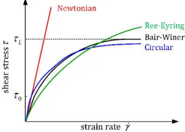
3.2 Lubricant rheological models . . . 25
3.3 Methodology. . . 27
3.3.1 Relative friction coefficient . . . 27
3.3.2 Numerical solution . . . 28
3.4 Time-dependent solution . . . 29
3.5 Effect of operating conditions . . . 34
3.6 Effect of surface anisotropy . . . 38
3.6.1 Longitudinal and transverse wavy cases. . . 38
3.6.2 Purely longitudinal wavy case. . . 41
3.7 Conclusion. . . 43
4 Friction of complex rough surfaces 44 4.1 Introduction . . . 44
4.2 Power spectral density friction method . . . 44
4.2.1 PSD friction model . . . 44
4.2.2 Model validation . . . 46
4.3 The artificial surface roughness. . . 47
4.3.1 Surface roughness power spectrum . . . 47
4.3.2 Friction increase prediction of a rough surface. . . 48
4.3.3 Comparison between the EHL simulation and the PSD prediction . . . 50
CONTENTS
4.4.1 Friction prediction under a specific operating condition . . . 54
4.4.2 Operating condition effects . . . 57
4.4.3 Friction curves for measured surface roughness . . . 59
4.5 Conclusion. . . 63
5 Conclusion and perspective 64 5.1 Conclusion. . . 64
5.2 Perspective. . . 65
Appendix A Construction of the coarse grid operator 66 Appendix B Derivation of matrix Ajfor line relaxation 71 B.0.1 Gauss-Seidel line relaxation. . . 71
B.0.2 Jacobi distributive line relaxation . . . 72
Appendix C Derivation of the scaling parameterθ2 74
Appendix D The relation between the elastic deformation and corresponding pressure
for 2D wavy surfaces 75
List of Figures
1.1 World primary energy consumption (red column: Non-OECD, blue column: OECD).
(Source: IEEJ Outlook 2019 and Scenario). . . 2
1.2 The variation of mean global surface temperature relative to 1880-2017. (Source: NASA/GISS) . . . 2
1.3 Total consumption by End-Use Sector, from 2000 to 2017. (Source: Data from the U.S. Energy Information Administration) . . . 2
1.4 Pressure flow factors. (Source: Reference [21]) . . . 4
1.5 Relative amplitude as a function of ∇2under pure rolling, where ∇2is dimension-less wavelength parameter, Ai and Ad are amplitude of surface roughness and deformed surface roughness respectively. (Source: Reference [58] ) . . . 5
1.6 Results obtained from measurements compared with theoretical attenuation curve defined by [56]. (Source: Reference [61] ) . . . 5
1.7 Friction coefficient versus speed for different loads. (Source: Ref. [83]) . . . 7
2.1 Mesh point (xi, yj) and it’s related mesh region ri , j . . . 13
2.2 Mesh point (i , j ). . . . 14
2.3 Interpolation process (green points: coarse grid points, black dots: fine grid points, blue dots: middle points on the fine grid, red point: central point on the fine grid). 17 2.4 Weighting factors for the interpolation (blue points: coarse grid points, black dots: fine grid points). . . 17
2.5 Flow chart of the hybrid relaxation process . . . 22
2.6 Implementation of the Multi-Grid method with a two level "V" cycle. . . 23
2.7 The time-dependent "V" cycles . . . 24
3.1 Shear stress-shear rate relationship for the EHL contact. . . 26
3.2 Comparison of the relative deformed amplitude (Ad /Ai ) as a function of f (r )∇2 for the current model (blue squares) with those on Reference [53] (solid line) . . 29
3.3 Top view of the surface waviness withλ/ah= 0.5 and Ai = 0.5Hc: (a) the isotropic surface waviness r = 1, (b) the longitudinal surface waviness r = 2, (c) the trans-verse surface waviness r = 0.5. . . . 30
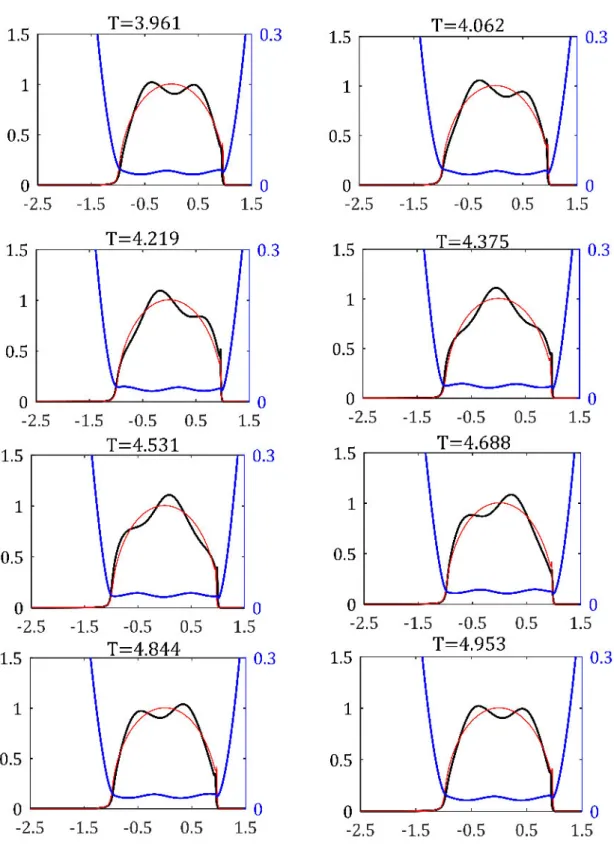
3.4 Central line pressure P (X , 0) (black lines) and central line film thickness H (X , 0) (blue lines) of isotropic surface waviness (r = 1) for M = 1000, L = 10, λ/ah= 0.5 and Ai = 0.5Hc during a time period. The central pressure line (red line) for the smooth case is plotted as a reference. . . 31
3.5 Central line pressure P (X , 0) (black lines) and central line film thickness H (X , 0) (blue lines) of longitudinal surface waviness (r = 2) for M = 1000, L = 10, λ/ah= 0.5 and Ai = 0.5Hc during a time period. The central pressure line (red line) for the smooth case is plotted as a reference. . . 32
3.6 Central line pressure P (X , 0) (black lines) and central line film thickness H (X , 0) (blue lines) of transverse surface waviness (r = 0.5) for M = 1000, L = 10, λ/ah= 0.5 and Ai = 0.5Hc during a time period. The central pressure line (red line) for the smooth case is plotted as a reference. . . 33
LIST OF FIGURES
3.7 The dimensionless central film thickness H croughas a function of the
dimension-less time T for: M = 1000, L = 10, λ/ah= 0.5 and Ai = 0.5Hc: (a) the isotropic
surface wavy case, (b) the longitudinal surface wavy case r = 2, (c) the transverse surface wavy case r = 0.5. . . . 34
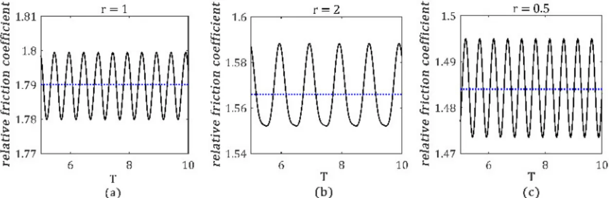
3.8 The relative friction coefficientµr/µs as a function of the dimensionless time T for: M = 1000, L = 10, λ/ah= 0.5 and Ai = 0.5Hc: (a) isotropic surface wavy case,
(b) longitudinal surface wavy case r = 2, (c) transverse surface wavy case r = 0.5. (Blue dotted line: average value of the relative friction coefficient.) . . . 34
3.9 Relative friction coefficient as a function of H c/Ai for a specific operating condition 35
3.10 Effect of the load parameter M on the relative friction coefficient for L = 10 and
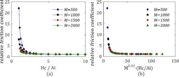
λ/ah= 0.5: (a) relative friction coefficient as a function of Hc/Ai , (b) relative fric-tion coefficient as a funcfric-tion of M0.33· (Hc/Ai ) . . . 35
3.11 Effect of material parameter L on the relative friction coefficient for M = 2000 andλ/ah= 0.5: (a) relative friction coefficient as a function of Hc/Ai , (b) relative friction coefficient as a function of L−1.1· (Hc/Ai ) . . . . 36
3.12 Effect of wavelengthλ/ah on the relative friction coefficient for M = 1000 and
L = 10: (a) relative friction coefficient as a function of Hc/Ai , (b) relative friction
coefficient as a function of (λ/ah)0.67· (Hc/Ai ). . . 36
3.13 Relative friction coefficient as a function of the classical parameter "lambda ratio" i.e. H c/Ai for a large range of operating conditions. . . . 37
3.14 Relative friction coefficient as a function of the new parameterθ2, simulation
re-sults: black circles; fitted curve: the black dashed line. . . 38
3.15 Relative friction coefficient (µr/µs) as a function of H c/Ai for different r (1 ≤ r ≤ 32) values for: M = 1000, L = 10 and λy/ah= 0.5 (left), zoom from 2.3 − 2.7 (right). 38
3.16 Relative friction coefficient (µr/µs) as a function of ff(r ) · (Hc/Ai ) for different r (1 ≤ r ≤ 32) values for: M = 1000, L = 10 and λy/ah= 0.5.. . . 39
3.17 Relative friction coefficient (µr/µs) as a function of (H c/Ai ) for different r (0 ≤
r ≤ 1) values for: M = 1000, L = 10 and λx/ah= 0.5(upper), zoom from 2.4 − 2.6
(lower). . . 40
3.18 Relative friction coefficient (µr/µs) as a function of ff(r ) × (Hc/Ai ) for different r (0 ≤ r ≤ 1) values for: M = 1000, L = 10 and λx/ah= 0.5. . . 40
3.19 ff (r ) as a function of r . Numerical results: red squares. Fitted curve: solid lines. . 41
3.20 Comparison between the transient relative friction coefficient and that of the sta-tionary case. Transient results: black line. Stasta-tionary results: magenta dash-dotted line. . . 41
3.21 Relative friction coefficients for the purely longitudinal wavy case: (a) relative fric-tion coefficient as a funcfric-tion of original "lambda ratio" H c/Ai parameter, (b) rel-ative friction coefficient as a function of the new parameterθ∗2 . . . 42
4.1 Flow chart for the relative friction coefficient prediction . . . 46
4.2 Surface roughness (a) and its 2D power spectral density (b) . . . 47
4.3 Power spectral density Ci soof the self-affine surface(Figure 4.2(a)) with H = 0.8.. 48
4.4 The selected artificial surface roughness (a), amplitude distribution of this sur-face roughness (b) and its power spectral density (c). . . 48
4.5 The ratio of the deformed amplitude and the initial amplitude fitted as Equation (3.17) (a) and the deformed surface roughness in frequency domain (b). . . 49
4.6 Comparison between the initial surface roughness (a) and the deformed surface roughness (b). . . 49
LIST OF FIGURES
4.8 Shear stress distributions for the smooth case (a) and for the rough case (b). . . . 50
4.9 The generated surface roughness patch (a), the roughness patch in the high pres-sure zone (b) and the periodical roughness pattern for full the numerical simula-tion (c). . . 50
4.10 Top view of the deformed surface roughness for a specific time step for a full nu-merical simulation (a) and for a PSD prediction (b). Central line r rd(x, 0) of the deformed surface roughness for the full numerical simulation (c) and for the PSD prediction (d). Central line p(x, 0) of the pressure distribution for the full numer-ical simulation (e) and for the PSD prediction (f ). . . 51
4.11 The relative friction as a function of dimensionless time employing the surface roughness pattern in Figure 4.9 (c) for the full numerical simulation method. . . 52
4.12 Top view of the twenty generated artificial random rough surfaces from N◦1 to
N◦20 with a same standard divation valueσ = 0.05µm and a same set of operating conditions listed in Table 4.1. . . 53
4.13 Measured surface roughness dART: (a) corrected surface roughness and (b) raw surface roughness. . . 54
4.14 Effective prediction areas. . . 55
4.15 An extracted surface patch of dART: (a) surface roughness height of this surface patch; (b) deformed surface patch; (c) pressure fluctuation of the surface patch.. 55
4.16 Extracted 529 surface patch (left) and their relative friction coefficient values (right). 56
4.17 Corrected relative friction coefficient values for 528 surface patches (left) and its histogram (right). . . 56
4.18 Relative friction coefficient as a function of total number of surface patches under the operating condition in Table 4.4.. . . 57
4.19 A extracted surface patch (left) and its average initial amplitude as a function as q. 57
4.20 The deformed surface patch shown in Figure 4.19 (left) and its pressure variations for case 1.. . . 58
4.21 The deformed surface patch shown in Figure 4.19 (left) and its pressure variations for case 2.. . . 58
4.22 The deformed surface patch shown in Figure 4.19 (left) and its pressure variations for case 3.. . . 58
4.23 The deformed surface patch shown in Figure 4.19 (left) and its pressure variations for case 4.. . . 58
4.24 The deformed surface patch shown in Figure 4.19 (left) and its pressure variations for case 5.. . . 59
4.25 Moes parameters M and L as a function of urfor the roughness dART. . . 59
4.26 The relative friction coefficient as a function of urfor the roughness dART. . . 60
4.27 The relative friction coefficient as a function of "Λ ratio" for the roughness dART. 60
4.28 Surface roughness dARTEb (left) and the top view of this roughness (right). . . . 60
4.29 Moes parameters M and L as a function of the rolling speed for the surface rough-ness dARTEb. . . 61
4.30 The relative friction coefficient as a function of urfor the surface roughness
dAR-TEb. . . 61
4.31 The relative friction coefficient as a function of the "Λ ratio" for the surface rough-ness dARTEb. . . 62
4.32 The relative friction coefficient as a function of the rolling speed urfor the surface
LIST OF FIGURES
A.1 Influences of the coarse grid operator Lhon central point, east point and north-east point. . . 67
A.2 Influences of the injection operator JhHon nine coincidental points (blue points). 69
D.1 Pressure distribution and the corresponding elastic deformation. . . 75
D.2 Amplitude of the elastic deformation ADd as a function of initial pressure ampli-tude Api for the following cases: (a) isotropic, (b) purely transverse, (c) purely lon-gitudinal. . . 76
D.3 Amplitude of the elastic deformation ADd as a function of wavelengthλ (λ = min(λx,λy)) for the following cases: (a) isotropic, (b) purely transverse, (c) purely longitudinal. 76
D.4 Amplitude of the elastic deformation ADd as a function of anisotropy parameter
List of Tables
1.1 U.S. CO2emissions from end-use sectors, 2008-2017. (Source: U.S. Energy
Infor-mation Administration, August 2018 Monthly Energy Review). . . 3
3.1 Relative friction coefficient versus the number of mesh points for: M =1000, L=10, λx/ah= 0.5, r=0.4 and Hc/Ai = 2. . . . 29
3.2 Relative friction coefficient versus different surface anisotropy parameters for: M = 1000, L = 10, λy/ah= 0.5 and Hc/Ai = 2. . . . 42
4.1 Operating condition parameters. . . 46
4.2 Relative friction coefficients as a function of the mesh points for two prediction schemes. . . 47
4.3 The relative friction coefficient obtained by EHL simulation and PSD prediction for 20 artificial random rough isotropic surfaces. . . 53
4.4 Measured operating condition and lubricant parameters. . . 55
4.5 Operating conditions of selected cases. . . 57
Nomenclature
Ad dimensionless deformed amplitude in the center of the contact
Ai dimensionless initial amplitude
ah the radius of the contact area ah=p3wR3 x/(2E0) m
C2D 2d power spectral density m4
Ci so 2d power spectral density of an isotropic surface m4
E1, E2 elastic moduli of the two contact bodies Pa
E0 reduced modulus of elasticity 2/E0= (1 − v2
1)/E1+ (1 − v22)/E2 Pa
f the friction force induced by the shearing of the lubricant N
F the dimensionless friction force
G dimensionless material parameter G = αE0
Ge elastic shear modulus Pa
G∞ the limiting elastic shear modulus Pa
h film thickness m
H dimensionless film thickness H = hRx/ah2
h0 mutual approach m
H0 dimensionless mutual approach
hc central film thickness m
H c dimensionless central film thickness for a smooth case H c = hcRx/a2h
H crough dimensionless central film thickness for a rough case
hx, h y dimensionless mesh sizes on the fine grid H x, H y dimensionless mesh sizes on the coarse grid IHh interpolation operator
IhH restriction operator
Lx, Ly lengths of final topography m
Ll coarse grid operator on the l th level
L dimensionless material parameter (Moes) L = G(2U )0.25
LIST OF TABLES
p pressure Pa
ps pressure for smooth cases Pa
ph Hertzian pressure Pa
δp pressure fluctuations Pa
∆P dimensionless pressure fluctuations∆P = δp/ph
qx, qy wavenumbers in x and y directions respectively 1/m
qr roll-off wavenumber 1/m
Rq root mean square of the surface roughness m
Rx reduced radius of curvature in x : 1/Rx= 1/R1x+ 1/R2x m
Ry reduced radius of curvature in y : Ry= Rx m
r wavelength ratio used to describe the surface anisotropy r = λx/λy
r r undeformed surface roughness m
r rd deformed surface roughness m
RR dimensionless surface roughness RR = r r · Rx/a2h
SRR slide to roll ratio
t time s
T dimensionless time T = t ¯u/ah
∆T dimensionless time step
u1, u2 velocities of lower surface and upper surface respectively m/s
ur mean velocity of contact surfaces ur= 0.5 × (u1+ u2) m/s
U dimensionless speed parameter U = (η0ur)/(E0Rx)
∆U slide-to-roll ratio∆U = δu/ur= (u1− u2)/ur
Urat slip parameter Urat= u1/ur
v1, v2 Poisson ratios of the two contact bodies
w normal load N
W2 2d dimensionless load parameter W2= w/(E0R2x)
x coordinate in the rolling direction m
X dimensionless coordinate X = x/ah
y coordinate perpendicular to x m
LIST OF TABLES
z pressure viscosity index
α pressure viscosity index 1/Pa
¯
α dimensionless viscosity index ¯α = αph
τ shear stress induced by the shearing of the lubricant Pa
τ0 the Eyring stress Pa
τL the limiting shear stress Pa
∇2 dimensionless wavelength parameter ∇2= (λ/ah)
p
M /L
¯
λ dimensionless speed parameter
λt the time constant for the fluid
λx,λy wavelength in x, y direction m
η viscosity Pa · s
η0 the atmospheric viscosity Pa · s
¯
η dimensionless viscosity ¯η = η/η0
ρ density of the lubricant Kg · m−3
ρ0 atmospheric density of the lubricant Kg · m−3
¯
ρ dimensionless density ¯ρ = ρ/ρ0
θ2 dimensionless new lambda ratio parameter
θ∗
2 dimensionless new lambda ratio parameter for purely longitudinal rough surfaces
˙
γ strain rate 1/s
µ friction coefficient
σ standard deviation of surface roughness m
Abbreviations
ART Amplitude Reduction Theory EHL Elastohydrodynamic Lubrication FFT Fast Fourier Transform
PSD Power Spectral Density
Superscripts
d deformed
h the fine grid
LIST OF TABLES i so isotropic l the l th level Subscripts a, b inlet, outlet i , d initial, deformed r, s rough, smooth st start x, y space domain qx, qy frequency domain
Chapter 1
Introduction
Contents
1.1 Background . . . . 1 1.2 Literature review . . . . 3
1.2.1 Methods to solve the rough contact problem. . . 3
1.2.2 Friction in rough EHL contact problem . . . 6
1.3 Research aims and Outlines. . . . 8
1.3.1 Research aims . . . 8
1.3.2 Outlines . . . 9
1.1 Background
Energy is the most important of all resources, which is needed to support economic and so-cial progress and build a better quality of life. According to the report of IEEJ Outlook 2019 (Institute of Energy Economics, Japan), the world primary energy consumption will continue growing from 2018 to 2050. Most of this growth comes from non-OECD (non-Organization for Economic Cooperation and Development) countries, where demand is driven by strong eco-nomic growth (shown in Figure1.1). Fossil energy like oil, coal and natural gas are still the largest energy source of the world, and the reserves of fossil energy are limited. Meanwhile, the over-consumption of fossil fuel leads to the over-release of carbon dioxide (CO2), methane,
oxynitride (NOx) and particulates into the air, which disturb the natural balance of the
atmo-sphere. The rapid rise in the carbon dioxide contributes to the serious global warming problem. NASA (National Aeronautics and Space Administration) reported that the global surface tem-perature has been persistently increasing since the late 19th century (shown in Figure1.2). An investigation from the U.S. Energy Information Administration (EIA) shows that the industrial and transportation sectors have consumed the most energy (shown in Figure1.3) as well as produced the most CO2emissions (show as Table1.1).
However, a substantial amount of energy is not put to useful purposes. Researches [1–4] show that a considerable amount of energy in industrial and transportation is consumed to overcome friction. For instance, energy consumed to overcome friction over the total energy consumption in heavy-duty vehicles is 33%, in paper machines is 32%, in passenger cars is 33% and in mineral mining industry is 40%. Recently, the increasing environment awareness requires efforts to improve energy efficiency and reduce CO2production. Correct lubrication
between engineering provides sufficient separation of the roughness present on the contact surfaces, which contributes to reducing friction losses. Better understanding and control of friction in mechanical components has the potential to offset large energy savings and CO2
emission reduction [5]. Studies [6–8] estimated that with the implementing advanced tribolog-ical technologies, such as using new contact surface, materials, lubricants, energy losses due to friction and wear could potentially be reduced by 40% in the long term (15 years) and by 18% in the short term (8 years )and CO2emissions globally can also reduced by 1,460 MtCO2(million
CHAPTER 1. INTRODUCTION
Figure 1.1: World primary energy consumption (red column: Non-OECD, blue column: OECD). (Source: IEEJ Outlook 2019 and Scenario)
Figure 1.2: The variation of mean global surface temperature relative to 1880-2017. (Source: NASA/GISS)
Figure 1.3: Total consumption by End-Use Sector, from 2000 to 2017. (Source: Data from the U.S. Energy Information Administration)
Hence, understanding the mechanisms of friction and improving frictional behavior be-tween engineering contact surfaces still remains an important issue in today’s research, not
CHAPTER 1. INTRODUCTION
only for meeting the increasing requirements of energy efficiency and CO2 emissions
reduc-tion but also for providing a theoretical tool in element design and optimizareduc-tion.
Table 1.1: U.S. CO2emissions from end-use sectors, 2008-2017. (Source: U.S. Energy
Informa-tion AdministraInforma-tion, August 2018 Monthly Energy Review) Units: million metric tons
year end-use sector 2008 2009 2010 2011 2012 2013 2014 2015 2016 2017 transportation 1898 1832 1848 1817 1779 1805 1823 1848 1886 1902 industrial 1608 1400 1508 1498 1489 1508 1511 1456 1428 1409 residential 1234 1127 1210 1149 1043 1100 1115 1037 982 956 commercial 1075 1007 1025 990 932 958 970 932 894 875
1.2 Literature review
Elastohydrodynamic lubrication (EHL) is the type of lubrication for frictional pairs having elas-tic contact under very high pressure and forming lubricant film in non-conformal contacts, such as rolling bearings, gears, human synovial joints and so on [9]. Lubricant film and sur-face roughness play an important role for improving reliability and effectiveness of mechanical parts as well as reducing friction losses. The majority of the published work on the influence of surface roughness on friction has been experimental, the minority of theoretical work has been done on friction prediction. This section represents the literature review on the methods to solve the rough EHL contact problem as well as friction in rough EHL contacts.
1.2.1 Methods to solve the rough contact problem
Typically, the EHL model consists of five equations [10], in which the Reynolds equation Equa-tion1.1is a partial differential equation and the film thickness equation Equation1.2contains an integral term, both equations are required to be solved simultaneously, making these equa-tions very complex. There are many approaches that can be used to solve this EHL model: the inverse method [11], the Newton-Raphson method [12], the homotopy method [13], the finite element method [14], the Multigrid method [15,16] and the Navier-Stokes approach [17]. So far, the Multigrid algorithm has been considered as one of the most efficient methods and applied frequently to EHL problems.
∂ ∂x( ρh3 12η ∂p ∂x) + ∂ ∂y( ρh3 12η ∂p ∂y) − ur ∂(ρh) ∂x = 0 (1.1) h(x, y) = h0+ x2 2 + y2 2 − r r (x, y) + 2 π2 Z +∞ −∞ Z +∞ −∞ P (x0, y0) p(x − x0)2+ (y − y0)2d x 0d y0 (1.2)
Where p represents the pressure, h denotes the film thickness, h0is the mutual approach and
ur = (u2+ u2)/2 is the mean velocity of two contact surfaces. ρ and η are the density and
vis-cosity of the lubricant, respectively. The x axis is aligned with the direction of the mean velocity ¯
u, and the y axis is perpendicular to the x direction.
In engineering, no surface is perfectly smooth, the order of magnitude of the surface rough-ness is often the same as or greater than that of the film thickrough-ness predicted by smooth contact conditions [18]. Therefore, the surface roughness should be considered. Generally, there are two methods to treat the rough lubrication problem numerically.
CHAPTER 1. INTRODUCTION
One approach is called the "stochastic" method. Early work was conducted on the hydrody-namic lubrication (HL) problem. Theoretical analysis of the implementation of the stochastic theory on rough HL contact problem was described by Christensen [19,20]. Then Patir and Cheng [21,22] proposed an average flow model to determine the effects of surface roughness on rough-lubricated contacts. In this model the Reynolds equation is simplified as an average Reynolds equation using a independent flow factor (shown in Figure1.4). Since the pioneering studies on the "average flow model", a number of authors have extended and generalized this work. Tripp [23] re-computed the flow factors using a perturbation expansion of the pressure in a nominal parallel film. When small roughness amplitude is considered, the flow factors calcu-lated in Reference [23] agree well with that of Patir and Cheng [21]. Hu and Zheng [24] studied the influence of boundary conditions, grid systems and statistics of rough surfaces on the flow factors. Lunde and Tonder [25] calculated the flow factors for an isotropic rough bearing and found that the boundary conditions of the selected bearing part can not affect the flow pass-ing through. Subsequently, Zhu and Cheng [26] extended the flow factors method in the point EHL contact problem. Some authors [27,28] applied the flow factors to deal with the cavitation problem. Letalleur et al. [29] studied the flow factors for two rough cases: smooth-rough sta-tionary case and rough-rough unstasta-tionary case. Sahlin et al. [30] developed a novel method using a homogenization technique to compute the flow factors. However, in stochastic model, roughness asperities are mainly treated as rigid.
Figure 1.4: Pressure flow factors. (Source: Reference [21])
Another way is to incorporate the surface roughness term r r (x, y, t ) in the film thickness equation (shown as Equation1.2) and to solve the system of equations directly. Due to the limitation of computation of speed and storage space, preliminary research [31–35] studied the steady state line rough contact problem, where the surface roughness is time-independent and one-dimensional model was considered. Later on, the stationary two dimensional rough contact problem [36–39] were carried out. With the increasing development of computational technique, transient cases were studied by many authors [40–51]. Based on the previous stud-ies on transient rough contact problem, Venner and Lubrecht et al. [52–60] published a series of papers on the "Amplitude Reduction Theory" describing the relation between the surface roughness deformation and operating conditions. They found that under very high pressure situations (piezoviscous elastic regime), the surface roughness will deform, and this
deforma-CHAPTER 1. INTRODUCTION
tion depends on operating conditions. A master curve (shown in Figure1.5) describes this relation quantitatively. Then ˇSperka et al. [61] verified the "Amplitude Reduction Theory" by measuring the deformed surface roughness on an optical test rig, the comparison of the mea-sured results and the predicted results can be found in Figure1.6. Recently, some extension work on the rough contact problem were addressed [62–65]. One of the most important studies about the influence of surface roughness on friction will be represented in the next subsection.
Figure 1.5: Relative amplitude as a function of ∇2under pure rolling, where ∇2is dimensionless
wavelength parameter, Ai and Ad are amplitude of surface roughness and deformed surface
roughness respectively. (Source: Reference [58] )
Figure 1.6: Results obtained from measurements compared with theoretical attenuation curve defined by [56]. (Source: Reference [61] )
The surface roughness term r r (x, y), which is often considered to be the same order of mag-nitude as the oil film thickness, incorporated in Equation1.2makes the coefficient (ρh3)/(12η) in the Reynolds equation jump orders of magnitude, which leads to a significant variation in EHL equations. From a mathematical point of view, the coefficient (ρh3)/(12η) is continu-ous, while in the numerical simulation, the coefficient causes a strong discontinuity in discrete
CHAPTER 1. INTRODUCTION
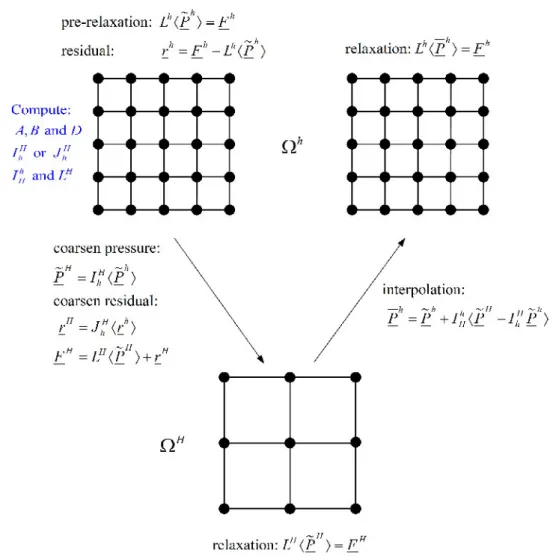
Reynolds equation. Work by Alcouffe et al [66] proposed an efficient way to overcome the above discontinuity through constructing the coarse grid in a Multi-grid code. The present work em-ploys the Multigrid techniques [10] to solve the rough contact problem. In addition, the idea provided by Alcouffe et al [66] is also applied to improve the code robustness and code effi-ciency.
1.2.2 Friction in rough EHL contact problem
Most heavily loaded machine elements are working under elastohydrodynamically lubricated conditions. Understanding the frictional behavior in such contacts plays an important role for reducing friction, preventing wear as well as improving service life. To reveal the relation be-tween fluid properties and friction, research has been conducted as follows: Crook [67] used a disc machine for measuring frictional traction. It was shown that the rolling friction (the trac-tion due to rolling) is independent of load and simply proportrac-tional to the film thickness in the elasto-hydrodynamic regime. Johnson and Cameron [68] measured traction in a rolling contact disc machine and results showed that the traction first increases and then decreases when the sliding speed increases. Johnson and Roberts [69] observed the visco-elastic behavior of film thickness through measuring shear forces on a rolling-contact test rig. Evans and Johnson [70] constructed traction maps depending upon pressure, temperature as well as shear rate for dif-ferent fluids, where difdif-ferent areas represent difdif-ferent traction behavior. Zhang et al. [71] stud-ied the elliptical contact between rib face and roller end in tapered roller bearings by means of a full numerical simulation. They found that the elastic deformation has a non-negligible influence on the friction coefficient. Yu and Medley [72] studied the influence of lubricant ad-ditives on friction via a side-slip disc machine. They concluded that the limiting shear stress, which is a useful parameter for predicting friction, is affected by the lubricant additives. Jacod et al. [73] predicted the coefficient of friction over a wide range of operating conditions and obtained a single generalized friction curve based on a full numerical simulation for a non-Newtonian EHL contact model. Vicente et al. [74] explored friction in rolling-sliding, soft-EHL contacts numerically and experimentally. Numerical calculations of the Couette friction are in good agreement with measured results. Very recently, Liu et al [75] calculated the friction co-efficient in a gear contact interface numerically, based on a thermal starved EHL model. They found that the maximum friction coefficient appears at the engaging-in point where a consid-erable slide-to-roll ratio exists. Björling et al. [76] measured the friction under EHL conditions on a ball-on-disc test rig for aged and fresh oils. Results showed that there is no difference in friction. In addition, Zhang [77] measured the EHL friction for a wide range of base fluids and compared the friction values for five different operating conditions. The study underlined the importance of molecular structure of the base fluid in determining the EHL friction.
Studies [78–80] showed that surface roughness has a significant impact on the friction be-havior of lubricated surfaces. A useful tool to investigate the frictional bebe-havior between rough surfaces is the classical Stribeck curve, showing the friction coefficient is a function of a ratio of the averaged oil film thickness to the combined surface roughness. The original research about the Stribeck curve dates back to the 19th century. In 1879, Thurston gave precise values of the friction coefficient and he was probably the first person to report that the friction coefficient passed through a minimum as the load increased [81,82]. Twenty years later, Stribeck [83,84] systematically published results of a carefully conducted and wide-ranging series of experi-ments on journal bearings, which are frequently referred to as ‘the Stribeck curve’ (shown in Figure1.7). G ¨umbel [85] organised Stribeck’s experimental results in a single curve by plotting the friction against the parameterηω/ ¯p, where η is the lubricant viscosity, ω is the angular ve-locity of the shaft and ¯p is the load per unit length. At the same time, Hersey [86] conducted
CHAPTER 1. INTRODUCTION
experiments on journal bearings and plotted the friction coefficient against the load, speed, temperature, viscosity and rate of oil supply. He showed that hydrodynamic friction should be a function ofηn/p in which n is the rotational speed and p is the pressure. Many years later, Wilson and Barnard [87] replotted the Stribeck curve by introducing a new variable i.e. zn/p, where the lower-case z stands for the lubricant viscosity. Subsequently, McKee [88] provided a similar dimensionless group Z N /P . Vogelpohl et al. [89] incorporated the boundary and fluid friction coefficient and showed a transition from the hydrodynamic lubrication regime to the mixed lubrication regime. All of the work mentioned above is performed under low pressure conditions, in the isoviscous rigid regime [90].
Figure 1.7: Friction coefficient versus speed for different loads. (Source: Ref. [83])
The situation for non-conforming contacts, such as those occurring in rolling element bear-ings, gears and cams, is somewhat different [91]. Shotter [92] experimentally showed that the friction increases with the surface roughness. Tallian and his co-workers [93,94] proposed a ratio |ξ0| between the elastohydrodynamic film thickness and the composite root mean square
roughness to represent the mixed elastodydrodynamic regime ( 1 < |ξ0| < 4 ). Poon [95] was
concerned with the transition from the boundary to the mixed regime with a dimensionless parameter 1 É ξ É 2 and the transition from mixed to full EHL region with 2 < ξ É 2.4 by using electrical-conductivity measurements. Bair and Winer [96] plotted the reduced traction coef-ficient as a function of a lambda ratio by performing sliding-rolling experiments. They found that when the lambda ratios is less than 2 the contact moves into the mixed regime. In gen-eral, the Stribeck curve can be divided into three regimes [97]: λ > 3 represents the full-film regime, 1 É λ É 3 is the mixed EHL regime and λ < 1 indicates the boundary regime. However, study [98] shows that this lambda ratio is not a suitable parameter to determine lubrication states especially when some aspects such as non-Newtonian, thermal and transient effects are considered. Transition locations from mixed to boundary lubrication regime or from full-film to mixed lubrication regime are still ambiguous. Therefore, an appropriate grouping including the speed, film thickness and roughness is required. Schipper [99] suggested a so-called Lu-brication number L0, which takes viscosity, speed and pressure into consideration, to detect the variation of the friction coefficient. Recently, Gelinck [100] extended Johnson’s model [101] to calculate the coefficient of friction for the whole mixed EHL regime. Lu and Khonsari [102]
CHAPTER 1. INTRODUCTION
examined the behavior of the Stribeck curve theoretically and experimentally on a journal bear-ing and found a good agreement. Wang et al. [103] presented a numerical approach developed on the basis of deterministic solutions of mixed lubrication to evaluate sliding friction. Mean-while, they measured the sliding friction on a commercial test rig. Both results were plotted against sliding velocities and also showed good agreement. Kalin [104] investigated changes of the Stribeck curve when one or two surfaces in the contact are non-fully wetted. After-wards, Kalin [105] tested the variations of the friction coefficient with diamond-like carbon coatings (DLC). Zhang [106] developed a numerical approach assuming the asperity interac-tion fricinterac-tion is proporinterac-tional to the contact area to predict the mixed EHL fricinterac-tion coefficient. Bonaventure [107] and his co-authors conducted rolling-sliding experiments with random sur-face roughness, they found that the onset of ML occurs at a higher entrainment productη0ue
(in whichη0 is inlet viscosity and ue is entrainment speed) and a relevant roughness scalar
parameter was obtained to predict the onset position.
Most of the work on Stribeck curve was done by experiments. Current study employs the Amplitude Reduction Theory [53] to study the frictional behavior in piezoviscous elastic regime [108] by means of numerical simulation.
1.3 Research aims and Outlines
1.3.1 Research aims
Long term successful operation of mechanical devices greatly depends on correct lubrication of the mechanical elements to provide sufficient separation of the roughness present on the contact surfaces. However, lubrication provides another important role, reducing friction be-tween rough contact surfaces.
The objective of the present research project is to develop an efficient and robust Multi-Grid-based algorithm to study the frictional behavior between rough contact surfaces. Current MultiGrid codes show the required efficiency, but are not sufficiently robust to treat the rough surface problem in a general way. Difficulties may lie in the following aspects:
(i) The efficient construction of the coarse grid of EHL Multi-Grid model to guarantee the code robustness and code efficiency of impact, rough surface EHL contact problems. (ii) Tests of the increased robustness of the new EHL Multi-Grid solver.
(iii) Implementation applied to test the code robustness and code efficiency of rough surface EHL contact problems.
(iv) The extension of the developed Multi-Grid lubrication code to transient contact prob-lems.
(v) The computation of the friction coefficient of rough contact surfaces.
(vi) The unification of friction curves that differ according to operating conditions.
(vii) The extension of the lambda ratio parameter predicting the transition from mixed to full-film regimes.
CHAPTER 1. INTRODUCTION
1.3.2 Outlines
According to the research aims listed in the previous sub-section. The layout of this thesis is as follows:
Chapter 1: This chapter first emphasizes the important role of friction played in energy
consumption and environmental issues. Subsequently, a literature review on the methods to solve rough contact problems and friction in rough contact problems is illuminated. The ob-jective and structure of the present thesis are given in the last section.
Chapter 2: This chapter represents the numerical model and algorithm for solving the
tran-sient rough EHL contact problem. The governing equations for trantran-sient EHL model are intro-duced first. Then the method proposed by Alcouffe et al [66] is employed to construct transfer operators as well as coarse grid operator. Finally the Multi-Grid method [10] is implemented.
Chapter 3: In this chapter, lubricant rheological models are illustrated in the first place. The
relative friction coefficient, an indicator for the full-film-mixed lubrication regime transition, is proposed in methodology section. Then the relative friction coefficient is calculated numer-ically for isotropic as well as anisotropic harmonic surface roughness respectively. Finally, a single friction curve is obtained using a new "lambda ratio" parameter.
Chapter 4: A rapid analytical prediction method using the power spectral density [109] is proposed to study a more complex surface topography in this chapter, firstly. Then an artificial surface roughness is employed to test this rapid prediction method. Finally, the prediction method is applied to predict friction for measured rough surfaces.
Chapter 5: The main results of current work are summarized and recommendations of
Chapter 2
Numerical model
Contents
2.1 Introduction . . . 10 2.2 Transient EHL model. . . 10
2.2.1 Governing equations . . . 10
2.2.2 Dimensionless equations and parameters . . . 11
2.3 The finite difference scheme . . . 13 2.4 Transfer operators . . . 15
2.4.1 Interpolation . . . 15
2.4.2 Injection . . . 18
2.5 Coarse grid operator . . . 20 2.6 Relaxation . . . 21 2.7 Implementation of the Multi-Grid method . . . 22 2.8 Conclusion . . . 24
2.1 Introduction
Multi-grid methods have been used successfully to treat Elastohydrodynamic lubrication (EHL) problems in the past [110–112]. However, when taking the surface roughness into account, film thickness and viscosity jump violently, both of them are strongly discontinuous parameters in discrete equations and will influence code robustness and code efficiency. The paper by R. Alcouffe [66] proposed an efficient way to solve this problem through constructing the coarse grid in a Multi-grid code. In this chapter, the Multigrid method is applied to solve the transient EHL model, and the algorithm outlined in Reference [66] is also implemented.
2.2 Transient EHL model
2.2.1 Governing equations
The lubrication of rough surfaces in EHL contacts is inherently a highly transient process. Study [40] shows that the surface roughness induced by the transient effect has a remarkable influence on the pressure and film thickness profiles. For the time-dependent problem [10], the Reynolds equation is given as:
∂ ∂x( ρh3 12η ∂p ∂x) + ∂ ∂y( ρh3 12η ∂p ∂y) | {z } poiseuille − ur∂(ρh) ∂x | {z } couette −∂(ρh) ∂t | {z } transient = 0 (2.1)
with p = 0 on the boundaries and the cavitation condition p Ê 0 everywhere. Where p is the pressure, h is the film thickness whose expression is shown as Equation2.2and ur= (u1+u2)/2
CHAPTER 2. NUMERICAL MODEL
direction of the x axis is as same as that of the mean velocity ur, the y axis is perpendicular to
x axis and t is time.
The equation used to describe the gap between the two contact bodies is the film thickness equation: h(x, y, t ) = h0(t ) + x2 2Rx+ y2 2Ry − r r (x, y, t ) + 2 πE0 Z +∞ −∞ Z +∞ −∞ p(x0, y0, t ) p(x − x0)2+ (y − y0)2d x 0d y0 | {z } elastic deformation (2.2)
in which r r (x, y, t ) stands for surface roughness. Rx and Ry represent the reduced radius of
curvature in x and y direction respectively. h0denotes the rigid body approach. E0is called the
reduced elastic modulus and its expression can be found below. The elastic deformation term is calculated with the approach named multilevel multi-integration [10,113].
2 E0 = 1 − v12 E1 + 1 − v22 E2
and E1and E2are the elastic moduli of the two contact bodies. v1and u2are the Poisson ratios.
In order to have a load balance. The integral of the pressure distribution should be equal to the applied load w .
Z +∞
−∞
Z +∞
−∞
p(x0, y0, t )d x0d y0= w(t ) (2.3) In the Reynolds equation (2.1),ρ is the density and η is the viscosity of the lubricant. Both of them are functions of pressure. A simply density pressure relation is given by Dowson and Higginson [114]:
ρ(p) = ρ0
5.9 × 10⁸+ 1.34p
5.9 × 10⁸+ p (2.4)
whereρ0 is the atmospheric density. The simplest viscosity pressure relation is proposed by
Barus [115]:
η(p) = η0exp(αp) (2.5)
in whichη0is the atmospheric viscosity andα is the pressure viscosity coefficient. However,
this exponential Barus equation usually predicts a higher viscosity value when the pressure is very large. A more realistic relation is derived by Roelands [116]:
η(p) = η0exp[(ln(η0) + 9.67)(−1 + (1 +
p p0
)z)] (2.6)
whereη0is the atmospheric viscosity and z is the pressure viscosity index, typically z = 0.6 and
p0= 1.98 × 10⁸Pa.
2.2.2 Dimensionless equations and parameters
To simplify the equation system and generalize the EHL model, the equations described above are made dimensionless using dimensionless variables based on the Hertzian dry contact solu-tion [117]. For the dry point contact case, the pressure distribution profile required for contact deformation reads:
p(x, y) =(php1 − (x/ah)
2− (y/a
h)2 if x2+ y2≤ a2h
CHAPTER 2. NUMERICAL MODEL
with ahthe radius of the contact area:
ah= 3
r 3wRx
2E0 (2.8)
and phis referred to as the Hertzian pressure:
ph=
3w
2πah2. (2.9)
Then the dimensionless variables are introduced to simplify the EHL model:
X = x/ah Y = y/ah P = p/ph H = hRx/a2h ¯ η = η/η0 ρ = ρ/ρ¯ 0 T = urt /ah α = αp¯ h (2.10)
Substituting the dimensionless variables in Equation2.1yields:
∂ ∂X( ¯ ρH3 ¯ η ¯λ ∂P ∂X) + ∂ ∂Y ( ¯ ρH3 ¯ η ¯λ ∂P ∂Y ) − ∂( ¯ρH) ∂X − ∂( ¯ρH) ∂T = 0 (2.11)
with X ∈ [Xa, Xb] and Y ∈ [−Ya, Ya]. Where ¯λ = (12urη0R2x)/(a3ph). And the boundary
condi-tions are P (Xa, Ya) = P(Xa, Y ) = P(Xb, Y ) = P(X ,Ya) = P(X ,−Ya) = 0. The cavication condition
is P (X , Y , T ) ≥ 0.
The dimensionless film thickness equation becomes:
H (X , Y , T ) = H0(T ) + X2 2 + Y2 2 − RR(X , Y , T ) + 2 π2 Z +∞ −∞ Z +∞ −∞ P (X0, Y0, T ) p (X − X0)2+ (Y − Y0)2d X 0d Y0 (2.12) where H0(T ) is determined by the dimensionless force balance equation:
Z +∞ −∞ Z +∞ −∞ P (X0, Y0, T )d X0d Y0=2π 3 (2.13)
The dimensionless density equation for a compressible lubricant reads:
¯
ρ(P) =5.9 × 10⁸+ 1.34phP
5.9 × 10⁸+ p hP
(2.14)
The dimensionless forms of viscosity equations are:
Barus: η = exp( ¯αP)¯ (2.15) and Roelands: η = exp((ln(η¯ 0) + 9.67)(−1 + (1 + ph p0 P )z)). (2.16) Beside the dimensionless variables mentioned in Equation2.10, two dimensionless numbers are often used to reduce the number of parameters, they are referred as Moes dimensionless parameters [118,119]. For point contact they are defined as [119]:
M = w E0R2 x (2η0ur E0Rx ) −3/4 (2.17)
CHAPTER 2. NUMERICAL MODEL
and
L = αE0(2η0ur
E0Rx )
1/4. (2.18)
For convenience, the Moes parameters can be used to re-write the parameters ¯α and ¯λ:
¯ λ = (128π 3 3M4 ) 1/3 ¯ α =L π( 3M 2 ) 1/3 (2.19)
Hamrock and Dowson [120] introduced three parameters to simplify the study of film thick-ness. For point contact they are written as:
W = w E0R2 x U =η0ur E0Rx G = αE0 (2.20)
2.3 The finite difference scheme
The second-order self-adjoint elliptic partial differential equation considered by Alcouffe [66] is
− ∇ · (D(x, y, t )∇U (x, y, t )) + σ(x, y, t )U (x, y, t ) = f (x, y, t ) (x, y) ∈ Ω (2.21) Compared to this equation, the Reynolds equation is of the same type with U = P, σ = 0, D = −( ¯ρH3)/(¯η ¯λ) and f = ∂( ¯ρH)/∂X + ∂( ¯ρH)/∂T . Rearranging the Reynolds equation (2.11) yields:
− ∂ ∂X(D ∂P ∂X) − ∂ ∂Y(D ∂P ∂Y) = ∂( ¯ρH) ∂X + ∂( ¯ρH) ∂T (X , Y ) ∈ Ω (2.22)
In the present work, the calculation domainΩ is a rectangle [Xa, Xb] × [−Ya, Ya]. This
do-main is covered with a uniform grids with a system of straight lines parallel to the coordinate axes. The mesh size in the two directions is hx = (Xb− Xa)/Nxand h y = 2×Ya/Ny, in which Nx
and Nyare the number of mesh points in both directions.
CHAPTER 2. NUMERICAL MODEL
To derive the difference scheme, a mesh region ri , j (shown as Figure2.1) defined by the
lines x = xi−hx/2 , x = xi+hx/2 , y = yj−hy/2 and y = yj+hy/2 for each mesh point (xi, yj) is
selected. In terms of each mesh point (xi, yj), P (xi, yj, tk) := Pi , j ,kis unknown, now integrating
Equation2.22over the corresponding mesh region ri , j:
− Z ri , j Z [ ∂ ∂X(D ∂P ∂X) + ∂ ∂Y(D ∂P ∂Y )]d xd y = Z ri , j Z [∂( ¯ρH) ∂X + ∂( ¯ρH) ∂T ]d xd y (2.23)
According to Green’s Theorem [121], Equation2.23can be expressed as:
− Z ci , j [(D∂P ∂X)d y − (D ∂P ∂Y)d x] = Z ri , j Z [∂( ¯ρH) ∂X + ∂( ¯ρH) ∂T ]d xd y (2.24)
where ci , jis the boundary of ri , jand the integration path along this boundary is anticlockwise.
Supposing f (xi, yj, tk) := fi , j ,k, the double integrals of the right hand side of Equation2.24can
be simply approximated by means of Z
ri , j
Z
f (x, y, t )d xd y= f. i , j ,k· ai , j. (2.25)
where ai , j= hx· h y is the area of the rectangle region ri , j shown in Figure2.2.
Figure 2.2: Mesh point (i , j ).
Referring again to Figure2.2, the line integal of Equation2.24over the four boundaries of
ri , j is approximated by means of central differences as:
− Z ci , j[(D ∂P ∂X)d y − (D ∂P ∂Y)d x] . = (h y)[Di +1/2,j,k( Pi , j ,k− Pi +1,j,k hx ) + Di −1/2,j,k( Pi , j ,k− Pi −1,j,k hx )] + (hx)[Di , j +1/2,k( Pi , j ,k− Pi , j +1,k h y ) + Di , j −1/2,k( Pi , j ,k− Pi , j −1,k h y )] (2.26)
CHAPTER 2. NUMERICAL MODEL
Rewriting Equation2.26and combining Equation2.25gives:
Ai , j ,k(Pi , j +1,k− Pi , j ,k)+Ai , j −1,k(Pi , j −1,k− Pi , j ,k)+ Bi , j ,k(Pi +1,j,k− Pi , j ,k) + Bi , j −1,k(Pi −1,j,k− Pi , j ,k) = Fi , j ,k (2.27) where Ai , j ,k= −( 1 2)( hx h y)(Di , j ,k+ Di , j +1,k) Bi , j ,k= −( 1 2)( h y hx)(Di , j ,k+ Di +1,j,k) Fi , j ,k= (hx · h y) fi , j ,k
In terms of fi , j ,k, the same discrete schemes used in Reference [10] is adopted. At this point,
the right hand side of Equation2.27can be taken as:
Fi , j ,k= h y(1.5 ¯. ρi , j ,kHi , j ,k− 2 ¯ρi −1,j,kHi −1,j,k+ 0.5 ¯ρi −2,j,kHi −2,j,k)
+hx · hy
ht (1.5 ¯ρi , j ,kHi , j ,k− 2 ¯ρi , j ,k−1Hi , j ,k−1+ 0.5 ¯ρi , j ,k−2Hi , j ,k−2)
(2.28)
where ht is the mesh size in time domain. A more detailed derivation of the above difference scheme can be found in Reference [122].
2.4 Transfer operators
Intergrid transfers are used for connecting the fine grid with the coarse grid. After a number of relaxations the error on the fine grid is smooth enough to be approximate on the coarse grid. Hence a restriction operator IhH is needed to transfer the approximated solutionPe
h
and the residual rh. When the low frequency errors have been eliminated on the coarse grid, it is necessary to define a new errorυh (υh= Ph− ePh) on the fine grid to correct the fine grid approximate solutionPe
h
. The classical bi-linear interpolation works quite well for most load cases. However when D jumps by orders of magnitude, Alcouffe [66] proposed a more efficient interpolation operator and this type of operator allows D∇P to be continuous over the whole calculation domain and gives a more reasonable physical representation on the coarse grid [123].
2.4.1 Interpolation
Having defined the coefficients A and B in Equation2.27, it is time to define the interpolation operator. In matrix form, the interpolation can be represented as:
υh
= IHhυ
H (2.29)
whereυh andυH are the fine grid and coarse grid error vectors respectively. IHh is the interpo-lation operator and the superscripts h and H stand for the fine grid and the coarse grid respec-tively. The new coarse grid construction method proposed by Alcouffe et al. [66] is used here, the interpolation process will be illustrated as follows:
The first step is to interpolate the fine grid points (black points shown in Figure2.3(b)) coin-ciding with the coarse grid points (green points shown in Figure2.3(a)):
υh
i F, j F,k= υ H
CHAPTER 2. NUMERICAL MODEL
whereυhis the error on the fine grid, andυHis the error on the coarse grid. Subscripts (i F, j F, k) and (iC , jC , k) are applied for illustrate the mesh points on the fine grid and on the coarse grid at the kthtime step respectively.
The second step is to obtain the middle points, represented as blue dots in Figure2.3(c), on the fine grid. Along horizontal lines, the expression for middle points is:
υh
i F +1,j F,k=
(Bi F, j F,kh υHiC , jC ,k+ Bi F +1,j F,kh υHiC +1,jC ,k)
(Bi F, j F,kh + Bi F +1,j F,kh ) (2.31) A similar expression can be derived for vertical lines, which reads:
υh
i F, j F +1,k=
(Ahi F, j F,kυHiC , jC ,k+ Ahi F, j F +1,kυHiC +1,jC ,k)
(Ahi F, j F,k+ Ahi F, j F +1,k) (2.32) Finally, the central point represented as a red point in Figure2.3(d) on the fine grid, which is obtained as: υh i F +1,j F +1,k= (A h i F +1,j F +1,kυ h i F +1,j F +2,k+ A h i F +1,j F,kυ h i F +1,j F,k+ Bi F, j F +1,kh υhi F, j F +1,k+ Bi F +1,j F +1,kh υhi F +1,j F +1,k)/ (Ahi F +1,j F +1,k+ Ahi F +1,j F,k+ Bi F, j F +1,kh + Bi F +1,j F +1,kh ) (2.33)
The above pointwise description (from Equation2.30to Equation2.33) can be replaced by the matrix expression Equation2.29, in which the matrix is large and complex. A simply way to describe this matrix is by using a stencil notation. As was shown in Figure2.4, in the interpo-lation process, the stencil provides weighting factors for dividing the coarse grid value in point (iC , jC , k) to the coinciding fine grid point (i F, j F, k) as well as its 8 adjacent points. Observing those pointwise expressions, the contribution of the coarse grid point to the 9 corresponding fine grids can be written as a stencil IHh in Equation2.34.
IHh= NWi F, j F,kh Ni F, j F,kh N Ehi F, j F,k Wi F, j F,kh Ci F, j F,kh Ei F, j F,kh SWi F, j F,kh Si F, j F,kh SEi F, j F,kh (2.34) where Ci F, j F,kh = 1, Ni F, j F,kh = Ahi F, j F,k Ahi F, j F,k+ Ahi F, j F +1,k, E h i F, j F,k= Bi F, j F,kh Bi F, j F,kh + Bi F +1,j F,kh , Si F, j F,kh = Ahi F, j F −1,k Ahi F, j F −2,k+ Ahi F, j F −1,k, W h i F, j F,k= Bi F −1,j F,kh Bhi F −1,j F,k+ Bi F −2,j F,kh ,
CHAPTER 2. NUMERICAL MODEL
Figure 2.3: Interpolation process (green points: coarse grid points, black dots: fine grid points, blue dots: middle points on the fine grid, red point: central point on the fine grid).
Figure 2.4: Weighting factors for the interpolation (blue points: coarse grid points, black dots: fine grid points).
![Figure 1.6: Results obtained from measurements compared with theoretical attenuation curve defined by [56]](https://thumb-eu.123doks.com/thumbv2/123doknet/14529337.723328/26.892.225.668.665.943/figure-results-obtained-measurements-compared-theoretical-attenuation-defined.webp)