A stochastic and flexible activity based model for large population. Application to Belgium

(1)

RESEARCH OUTPUTS / RÉSULTATS DE RECHERCHE

Author(s) - Auteur(s) :

Publication date - Date de publication :

Permanent link - Permalien :

Rights / License - Licence de droit d’auteur :

Bibliothèque Universitaire Moretus Plantin

Institutional Repository - Research Portal

Dépôt Institutionnel - Portail de la Recherche

researchportal.unamur.be

University of Namur

A stochastic and flexible activity based model for large population. Application to

Belgium

Barthelemy, Johan; Toint, Philippe

Published in:

Journal of Artificial Societies and Social Simulation

Publication date:

2015

Document Version

Early version, also known as pre-print

Link to publication

Citation for pulished version (HARVARD):

Barthelemy, J & Toint, P 2015, 'A stochastic and flexible activity based model for large population. Application to Belgium', Journal of Artificial Societies and Social Simulation, vol. 18, no. 3.

General rights

Copyright and moral rights for the publications made accessible in the public portal are retained by the authors and/or other copyright owners and it is a condition of accessing publications that users recognise and abide by the legal requirements associated with these rights. • Users may download and print one copy of any publication from the public portal for the purpose of private study or research. • You may not further distribute the material or use it for any profit-making activity or commercial gain

• You may freely distribute the URL identifying the publication in the public portal ?

Take down policy

If you believe that this document breaches copyright please contact us providing details, and we will remove access to the work immediately and investigate your claim.

(2)

by J. Bathelemy and Ph. L. Toint

Report naXys-10-2013 October 29, 2013

Namur Center for Complex Systems

University of Namur,

61, rue de Bruxelles, B5000 Namur (Belgium) http://www.naxys.be

(3)

Johan Barth´

elemy

∗

, Philippe L. Toint

†

,

October 29, 2013

Abstract

The VirtualBelgium project aims at developing understanding of the evolution of the Belgian popula-tion using agent-based simulapopula-tions and considering various aspects of this evolupopula-tion such as demographics, residential choices, activity patterns, mobility, etc. This simulation is based on a validated synthetic pop-ulation consisting of approximately 10,000,000 individuals and 4,350,000 households localized in the 589 municipalities of Belgium.

The work presented in this paper focuses only on the mobility behaviour, simulated using an activity-based approach in which the travel demand is derived from the activities performed by the individuals. The proposed model is distribution based and requires only minimal information, but is designed for easily taking advantage of any additional network-related data available.

The proposed activity-based has been applied on the Belgian synthetic population. The quality of the agent behaviour is discussed using statistical criteria extracted from the literature and it is shown that VirtualBelgium produces satisfactory results.

Keywords Micro-simulation, agent based simulation, activity chains, transport demand forecasting, nationwide models

1 Introduction and motivation

Activity-based models form a class of travel demand forecasting model originally based on ideas by H¨agerstrand (1970) and Chapin (1974). These were proposed as an alternative to the classical four-stages trip-based models for travel demand forecasting, whose drawbacks were by then well identified (i.e. Dickey, 1983, Domencich and McFadden, 1975, Spear, 1977, Oppenheim, 1995). Activity-based approaches rely on the paradigm that people travel to carry out activities they need or wish to perform. Such models reflect the scheduling of activities performed by individuals in time and space and the sequence of activities, also names activity chains or activity patterns, becomes the relevant unit of analysis. This approach is now widely accepted and continues to attract a lot of attention.

Activity-based models can be classified in at least four families. The first two are discrete choice models (Adler and Ben-Akiva, 1979, Bhat and Koppelman, 1999, Bradley, Bowman and Griesenbeck, 2010 and Bhat, Guo, Srinivasan and Sivakumar, 2004) and mathematical programming techniques (Gan and Recker, 2008). They have the drawbacks that the former approach may requires an extremely large choice set in order to capture a sufficient fraction of feasible mobility patterns, while the latter may not be tractable as the decision processes’ formulation may be extremely complex. This last issue also appears in structural equation modelling techniques, another family of activity-based models, which is rather confirmatory than explanatory. We refer the reader to Golob (2003) for a review of contributions using this approach and to Hoe (2008) for an insight on its limitations. Finally, the fourth model’s family exploits the advent of high performance computing: it uses massive multi-agents micro-simulations in order to reproduce behaviours within a complex system, such as mobility behaviours of a large population (Kitamura, Chen and Pendyala (1997)).

It has been noted that that ”micro-simulation ... is drawing attention as a new approach to travel demand

forecasting” (Miller 1996), and several operational micro-simulators for activity scheduling are currently in

∗_{Namur Research Center for Complex Systems (NAXYS), FUNDP-University of Namur, 61, rue de Bruxelles, B-5000 Namur,}

Belgium. Email: [email protected]

†_{Namur Research Center for Complex Systems (NAXYS), FUNDP-University of Namur, 61, rue de Bruxelles, B-5000 Namur,}

Belgium. Email: [email protected] (corresponding author)

(4)

use. Examples include ALBATROSS (Arentze and Timmermans (2000)) for the Netherlands, TASHA (a part of the ILUTE simulator, Salvini and Miller (2005)) for the Greater Toronto Area, SAMS and AMOS (Kitamura et al. (1996)). A review and comparison of various micro-simulators and discrete choice models for activity-based modelling can be found in (Goran 2001). These approaches typically implement the first three steps (generation, distribution and modal choice) of the traditional four-stage model. The last step, namely traffic assignment, can be handled with dynamic traffic assignment procedures, whose adoption has been made easier by the the development of powerful open source agent-based simulation systems such as MatSim (see http://www.matsim.org, accessed on February, 2013), used by Meister et al. (2010) in travel demand forecasting for Switzerland, Urbansim (Waddell (2002)) and Transim (Nagel, Beckman and Barrett, 1999.

Even though all these approaches have demonstrated their usefulness, they typically requires, in addition to a complete description of the road network, an a-priori localisation of every housing unit, services, shops,... This turns out to be a strong requirement: indeed, if this information can often be gathered for a particular city or even a district of a country, the geo-localisation process is far more complex and cumbersome for a whole country and may be not feasible. This issue motivates our interest for the design of an alternative methodology obviating this limitation, but flexible enough to use every information available and making it suitable for a nationwide application.

The approach taken in this work is the micro-simulation of the Belgian population’s mobility behaviours as a part of the VirtualBelgium integrated simulator. The agents are derived from a synthetic population previously generated and validated (see Barthelemy and Toint, 2012, for a complete description of the synthetic population generator). The proposed activity scheduling model is a three steps procedure: first, a set of feasible activity chains is generated for every agent type; a chain is then assigned to every individual agent of the simulation using a randomized model; and all activities’ characteristics of the chain are finally determined based on statistical distributions. The outputs of the model can then processed using MATSim for dynamic traffic assignment, if required. VirtualBelgium’s activity-based models rely mainly on data extracted from the Mobel and Beldam national mobility surveys conducted in Belgium (Hubert and Toint (2002), ref Cornelis et al. 2012 ) and the OpenStreetMap project (Haklay and Weber 2008).

The remainder of this paper is organized as follows. Section 2 describes VirtualBelgium’s base architecture, data sources, agents and activity chains possibly performed by them. In Section 3, we detail the proposed method for assigning activity chains to individual agents. We next present in Section 4 the results obtained with this methodology when applied to VirtualBelgium. Concluding remarks and future perspectives are finally discussed in Section 5.

2 VirtualBelgium: a multi-agent micro-simulation for Belgium

Describing our activity chain generator is difficult without introducing the basic elements of the framework in which these patterns are exploited. We therefore start with a brief outline of VirtualBelgium, a research project for simulating mobility behaviour and demographic evolution of the Belgian population using a multi-agent approach, based on the Repast HPC (Collier and North (2012)) and MATSim frameworks. The agents of interest in VirtualBelgium consists of individuals in a population P = (I, H) of approximatively 10.000.000 people ∈ I gathered in 4.350.000 households ∈ H and localized in 589 municipalities. A consistent synthetic population for Belgium was generated using a sample-free generator (see (Barthelemy and Toint 2012) for a detailed description of the algorithm). Agent’s initial attributes, which significantly influence travel behaviour (Avery (2011), Hubert and Toint (2002), Cornelis et al. (2012)), are described in Tables 2.1 and 2.2. This work being focused on agent’s mobility behaviour, their evolution processes will not be discussed in this paper.

Attribute Values

Gender male; female

Age class 0-5; 6-17; 18-39; 40-59; 60+

Age an integer from 0 to 110

Socio-professional status student; active; inactive

Education level primary; high school; higher education; none

Driving license ownership yes; no

(5)

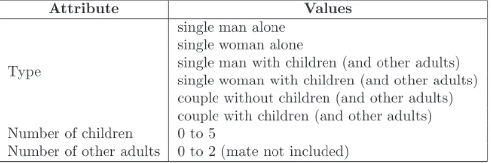
Attribute Values

Type

single man alone single woman alone

single man with children (and other adults) single woman with children (and other adults) couple without children (and other adults) couple with children (and other adults)

Number of children 0 to 5

Number of other adults 0 to 2 (mate not included) Table 2.2: Households’ characteristics

An overview of VirtualBelgium’s structure, which follows the standard of agent-based programming ap-proach (van Dam, Nikolic and Lukszo, 2012), is illustrated on the class diagram of Figure 2.1. The agents (Individual and Household classes), their actions and the interactions between them are ruled by a scheduler (belonging to the Model class). One tick of the simulation represents one day of activities scheduling by the agents. The agents’ environment is the Belgian road network (Network class).

Individual -id: int -household_id: int -household_relationship: char = H, M, C, A -gender: char = M, F -age_class: int = 0-4 -age: int = 0-104 -education_level: char = O, P, S, U -socio_professional_status: char = I, A, S -driving_licence: char = O, P -activity_chain: vector<Activity> +setActivityChain(): void Household -id: int -type: char = I, C, N, F -number_of_children: int = 0-5 -number_of_additional_adults: int = 0-2 -list individual: vector<int> -ins: int

-house_node_id: long = a network node id +localizeHouse(): void Activity -type: char = d, m, v, t, e, r, c, p, f, b, l, o -type_num: int = 1-12 -end_time: float -duration: float -distance: float -node_id: long composition schedule Network

-nodes: map<long, Node> -links: map<long, Link>

+getDestinationFromSource(source_id:long,distance:float): long localization localization Model -individual_agents: SharedContext<Individual> -household_agents: SharedContext<Household> -model properties: Properties

+step(): void +scheduler(): void agents agents Node -id: long -x: double -y: double -indicators: map<string,long> -links_out: vector<long> Link -id: long -start_node_id: long -end_node_id: long -lenght: float composition composition

Figure 2.1: Class diagram

2.1 Activity chains, general assumptions and data source

Activity chains data used by VirtualBelgium is derived from the Mobel 2001 and Beldam 2012 mobility surveys conducted in Belgium. These surveys highlighted 12 base activities:

(6)

d pick up or drop someone m staying home

v work related visit t work e school r eating outside c shopping p personal reason f visiting relatives b going for a walk l leisure activity o other

Each activity is also characterized by a duration and a localization, i.e. a node of Belgium’s road network, extracted from OpenStreetMap. Note that individual below 5 years old (included) are discarded as it is assumed that they always travel with their relatives and they don’t have proper activity chains.

An activity chain is then a sequence of these base activities. It is assumed that each activity chains begins and ends at the individual’s home. These concepts are formally described in Definition 1.

Definition 1 (Activity chain) An activity α performed by an individual is a quadruplet (αp_{, α}l_{, α}s_{, α}d_{) where}

• αp _{= the purpose ;}

• αl_{= the localization ;}

• αs_{= the starting time ;}

• αd _{= the duration ;}

of the activity. An activity chain α∗_{= (α}

n)n∈{1,...,k} of size k is then a sequence α1,· · · , αk of activities.

The variety of observed activity chains is significant, as approximately 10,000 different such chains have been extracted from the mentioned national surveys.

3 Activity chains generation and assignment

How to assign activity chains to each individual in the VirtualBelgium simulation? This section presents a proposal for performing this assignment which does not rely on the geo-localization of each of the potential activity sites, an information which is (unfortunately) missing in our context. We start by outlining the main steps of our approach before a more formal description.

The first step is to generate a set of feasible activity-chains for each individual type available. It is also required that every individual is assigned to a house localized in the network, a task which is necessary because the synthetic population generator only specifies the homes’ municipality. This house will be the starting and ending point of the activity chain for each individual living inside it. Once these preliminary steps have been performed, the assignment of a fully characterized activity chain to an individual consists in drawing an activity chain α∗ _{from the appropriate activity-chain set and finally determining the characteristics of every activity}

α∈ α∗_{. This methodology is fully described in the remainder of this Section.}

3.1 Generation of activity chains patterns by individual type

In our context, an individual is characterized by a vector of m attributes V = (V1, . . . , Vm), whose components

may take a discrete and ordered set of values (see Table 2.1). Let’s denote by TI, Ai and ni the set of all

individual type, the set of activity chain patterns that could be extracted from the data relative to i ∈ TI and

the size of Ai, respectively. Definition 2 introduces the concept of neighbourhood for an individual type by

shifting its attributes’ values.

Definition 2 (l-neighbourhood) For an individual type i and a integer l ∈ {1, . . . , m}, the l-neighbourhood

of i, denoted by Nl

i, is the set of all individual types obtained by at most l shifts between contiguous values of

the attributes of type i.

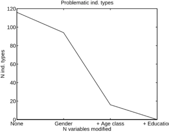
Depending on the data, the number of observed activity chains may be lower than a desired minimal threshold t for a subset of individual type TJ ⊆ TI. It is then necessary to add activity chains to the

problematic Aj such that the constraint

(7)

yields. We propose to augment Aj with the activity chains in Ak, where k ∈ Njl and l is as small as possible.

For VirtualBelgium, a threshold value t set to 5 has shown to produce reasonable diverse results. As one can observe in Figure 3.2, out of 192 individual types, 116 problematic classes were identified in the raw data and an at most a 3-neighbourhood was required to satisfy the constraint. In our implementation, the Nl

j (l = 1, 2, 3)

are generated by sequentially modifying the following attributes: 1. gender;

2. gender and age class;

3. gender, age class and education level.

None0 Gender + Age class + Education

20 40 60 80 100 120

Problematic ind. types

N variables modified

N ind. types

Figure 3.2: Numbers of problematic individual class with respect to the neighbourhood’s level.

3.2 Activity chains assignment

Once a set of activity chains Aiis available for each individual type i ∈ TI, the next step is to assign a chain to

every individual agent. This is done by randomly drawing an activity chain α in Aiif the considered individual

is of type i, using the empirical distribution obtained from the Mobel survey. For instance, Table 3.3 illustrates the set A of feasible activity chains and their respective weights for a student woman between 18 and 39 years old with a higher education degree and without a driving licence.

Pattern 2 5 10 2 2 9 2 2 5 2 2 5 2 10 2 2 5 6 5 2 2 11 2

Weight 0.272 1.025 0.913 0.412 0.412 0.284

Table 3.3: Weighted A for a given individual agent (Mobel).

3.3 Household’s house localization

As stated previously each household and its constituent members are already located in one of the 589 mu-nicipality. Nevertheless, as the goal is to locate an activity at network-node level, and no data is available at a more disaggregate level, the first part of the process consists in assigning each household to a node of their municipality’s road network. The node, randomly drawn following a discrete uniform distribution (in order to preserve the population density of the municipality), will be referred as the household’s house.

3.4 House departure time

The first step taken by an agent is to leave its home in order to perform the first activity of the day, i.e. a house departure time h must be determined. Regarding the activity type to be performed, the time departure

(8)

distribution H varies and is approximated by a mixture distribution which is fitted to the empirical distribution obtained from the Mobel survey. The mixture is of the form

H ∼ f (x | p) =

l

X

i=1

wiCi(x; µi, σ2i | p)

where p is the activity purpose, l the number of components, wi is the weight associated with the component

Ci such that wi≥ 0 andPiwi = 1. The Ciconsidered here follow a Log-Normal distribution LN (µi, σi2) with

location parameter µi ∈ IR and scale parameter σ2i. For a detailed description of such mixture distributions,

see McLachlan and Peel (2000).

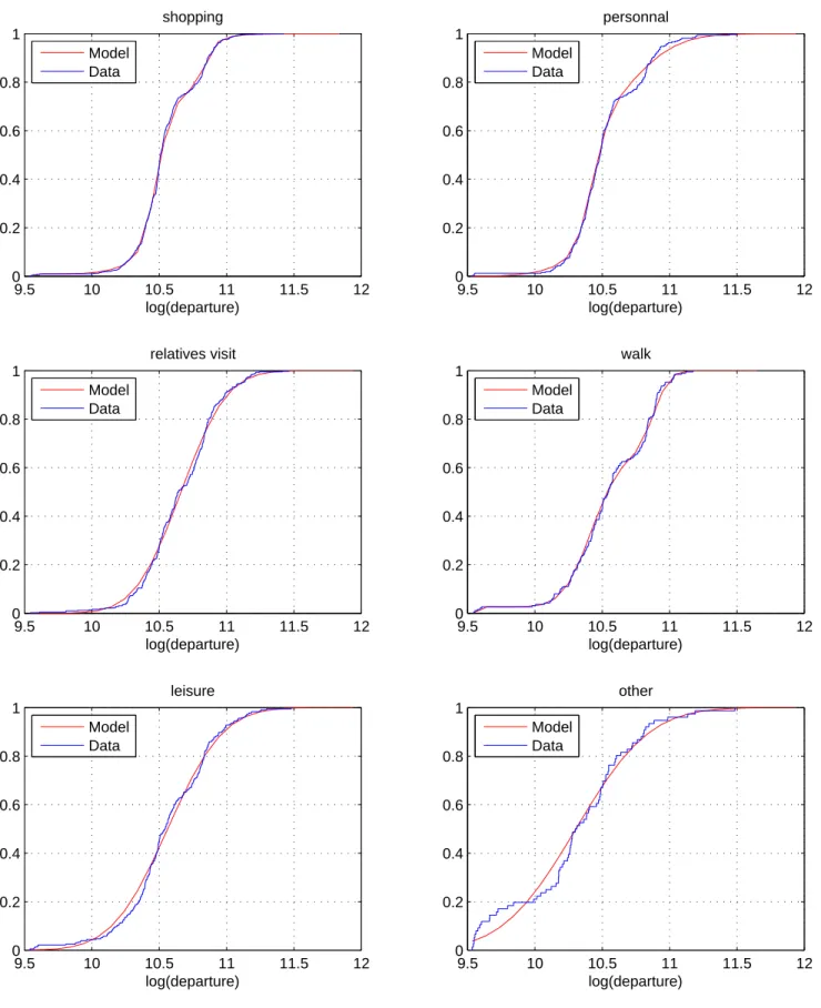
The empirical and fitted distributions are illustrated in Figures 3.3 and 3.4. It is important to note that the number of components is determined such that each mixture distribution obtained is statically similar to the empirical distribution according to the univariate Kolmogorov-Smirnov goodness-of-fit test (Massey, 1951) at 5% significance level.

The departure time is then randomly drawn accordingly to the appropriate distribution(1)_.

3.5 Activity localization

We now turn to the details of how the localization of an activity is determined inside the road network of Belgium. Given that each individual has a house, it is possible to localize each of his/her activities in the network, the house being the starting point of the activity chain. These activities will also take place at a node of the network, which is determined as follow:

1. a distance d is drawn from a distribution pertaining to the considered activity; 2. a set of nodes at distance d from the current localization is generated;

3. finally a node is drawn from the set generated at previous step. We now give more detail on these three steps.

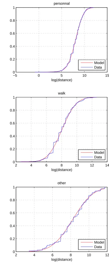
3.5.1 Random draw of a distance

Similarly to the house departure time, the random draw of the distance d travelled to perform an activity and follow a mixture of distribution conditional to the type of the activity chain which is fitted to the empirical distribution obtained from the Mobel survey. Empirical and resulting fitted probability density functions are illustrated in Figures 3.5 and 3.6.

3.5.2 Generation of a set of feasible nodes for a given activity

The next step is to generate a set of node at distance d from the current localization, at which the considered activity could take place. A Dijkstra algorithm relying on a Fibonacci heap data structure (Fredman and Tarjan, 1987), is then used to explore the network and find these feasible nodes. For a network with n nodes and m arcs, this algorithmic variant has the crucial advantage in our context of requiring O((n log n + m) operations, instead of O(n2_{) for a more direct implementation. If no suitable node is found at the desired distance, then}

the same procedure is applied but with a range of distances [d − ǫ, d + ǫ]. This error term ǫ is increased(2) _until

at least one node is discovered. 3.5.3 Activity node choice

If no additional data is available, the destination node αl_{is then randomly chosen from a discrete uniform draw.}

Otherwise, the draws can be empirically weighted in order to take information on specific activity localization at specific nodes/municipalities (for instance using geo- localization) into account. To illustrate our proposal,

(1)_{Directly drawing from empirical distribution has also been investigated, but this was up to 3 times slower in the conducted}

experiments. As a very large number of draws is involved (in the hundred of millions), random number generation speed becomes an essential issue to address and this approach has been discarded.

(9)

9.5 10 10.5 11 11.5 12 0 0.2 0.4 0.6 0.8 1 log(departure) pick up/drop someone Model Data 9.5 10 10.5 11 11.5 12 0 0.2 0.4 0.6 0.8 1 log(departure) home Model Data 9.5 10 10.5 11 11.5 0 0.2 0.4 0.6 0.8 1 log(departure) work visit Model Data 6 7 8 9 10 11 12 0 0.2 0.4 0.6 0.8 1 log(departure) work Model Data 9.5 10 10.5 11 11.5 12 0 0.2 0.4 0.6 0.8 1 log(departure) school Model Data 9.5 10 10.5 11 11.5 12 0 0.2 0.4 0.6 0.8 1 log(departure) eating outside Model Data

Figure 3.3: House departure time (minutes after midnight) : empirical and estimated cumulative distribution functions by purpose.

(10)

9.5 10 10.5 11 11.5 12 0 0.2 0.4 0.6 0.8 1 log(departure) shopping Model Data 9.5 10 10.5 11 11.5 12 0 0.2 0.4 0.6 0.8 1 log(departure) personnal Model Data 9.5 10 10.5 11 11.5 12 0 0.2 0.4 0.6 0.8 1 log(departure) relatives visit Model Data 9.5 10 10.5 11 11.5 12 0 0.2 0.4 0.6 0.8 1 log(departure) walk Model Data 9.5 10 10.5 11 11.5 12 0 0.2 0.4 0.6 0.8 1 log(departure) leisure Model Data 9.5 10 10.5 11 11.5 12 0 0.2 0.4 0.6 0.8 1 log(departure) other Model Data

Figure 3.4: House departure time (minutes after midnight) : empirical and estimated cumulative distribution functions by purpose.

(11)

2 4 6 8 10 12 14 0 0.2 0.4 0.6 0.8 1 log(distance) pick up/drop someone

Model Data −5 0 5 10 15 0 0.2 0.4 0.6 0.8 1 log(distance) home Model Data 2 4 6 8 10 12 14 0 0.2 0.4 0.6 0.8 1 log(distance) work visit Model Data 2 4 6 8 10 12 14 0 0.2 0.4 0.6 0.8 1 log(distance) work Model Data 0 2 4 6 8 10 12 0 0.2 0.4 0.6 0.8 1 log(distance) school Model Data 2 4 6 8 10 12 0 0.2 0.4 0.6 0.8 1 log(distance) eating outside Model Data

(12)

−5 0 5 10 15 0 0.2 0.4 0.6 0.8 1 log(distance) shopping Model Data −5 0 5 10 15 0 0.2 0.4 0.6 0.8 1 log(distance) personnal Model Data 0 5 10 15 0 0.2 0.4 0.6 0.8 1 log(distance) relatives visit Model Data 2 4 6 8 10 12 14 0 0.2 0.4 0.6 0.8 1 log(distance) walk Model Data 4 6 8 10 12 14 0 0.2 0.4 0.6 0.8 1 log(distance) leisure Model Data 2 4 6 8 10 12 0 0.2 0.4 0.6 0.8 1 log(distance) other Model Data

(13)

assume a road network and an activity choice resulting in a set of 4 feasibles nodes, whose indicators for 3 types of activity are detailed in Table 3.5.3 (nodes 1 and 2 belongs to the same municipality). If no indicators is available, such as for leisure, then the line is set to na; work is municipality-related indicator and school is a node-related indicator used for precise geo-localization of schools.

Indicator Node 1 Node 2 Node 3 Node 4

work 1000 1000 500 800

school 0 1 0 0

leisure na na na na

Table 3.4: Nodes’ indicators

The proposed technique has the advantage of using localization data whenever available, but also allows for a reasonable alternative, would such information be missing.

3.6 Activity duration

An activity duration depends on its starting time, which is obtained by adding the ending time of the previous activity and the trip duration performed to reach the current localization. The time spent to carry out an activity is then determined by

1. drawing a trip duration t to a compute a starting time αs_;

2. and drawing an activity duration αd _{conditional to s.}

These two steps are detailed in the remaining of this Section.

3.6.1 Trip duration and starting time

It is clear that a trip duration t is related to its distance d. This observation lead us to fit a mixture a bivariate distribution to approximate the joint-distribution of (D, T ) where T and D are respectively the random variables associated with the duration and the distance of the trip. The resulting bivariate distribution is illustrated in Figure 3.7 and is defined by

(D, T ) ∼ f (x) =

l

X

i=1

wiCi(x; µi,Σi)

were l the number of components, wi is the weight associated with the component Ci such that wi ≥ 0 and

P

iwi = 1. The Ci considered here follow a bivariate Log-Normal distribution LN (µi,Σi) with location vector

µi= (µ_i,1, µ_i,2)

and scale matrix

Σi =µσi,11 σi,12

σi,21 σi,22

¶ .

As for the distributions of the house departure time and the distance performed to reach an activity, the number of components l is determined in order to obtained a fitted distribution that is statistically similar to the empirical distribution according to the Fasano and Franceschini’s generalization of the Kolmorov-Smirnov goodness-of-fit test (Fasano and Franceschini, 1987) at significance level of 5%.

The fitted distribution is illustrated in Figure 3.7. As one could expect, there is a positive correlation between the distance and the duration of trip, i.e. the further an individual go, the more time he spend on the road. It can also be noted the variance of the duration is higher for smaller trip, and gradually decrease as the distance increase.

Since the distance d is computed in Section 3.5, it follows from (Eaton, 1983) that the trip duration t can be draw from the univariate conditional distribution of T given D = d defined by

T | D = d ∼ f (x |D = d) =

l

X

i=1

(14)

5 6 7 8 9 10 11 12 4 5 6 7 8 9 log(distance) log(duration) 0.02 0.04 0.06 0.08 0.1 0.12 0.14 0.16

Figure 3.7: Fitted probability density function of log(distance) (meters) × log(duration) (seconds) where l is the number of components, wiare the weights of the mixture and Ci follow a univariate Log-Normal

distribution LN (µi, σi) such that

µi= µi,2+ σi,12 σi,11 (d − µi,1) and σi= σi,22− (σi,12)2 σi,11 .

The starting time of αi∈ α∗(i > 1) is then obtained by adding the transportation duration and the ending

time of the previous activity of the chain, i.e. αsi = (α

s

i−1+ αdi−1) + t.

3.6.2 Activity duration

Since an activity duration is correlated with its starting time and purpose, the computation of αd _{follow a}

similar process applied for determining a trip duration, i.e. for each purpose the joint- distribution of an activity starting time and its duration is fitted to the data. Figure 3.8 and 3.9 illustrate the resulting joint-distributions, from which behavioural patterns can be observed. For instance

• individuals mainly start working at 8:30 for 9 hours, but the distribution also highlights the part-time worker starting at 8:30 or 13:00;

• students usually start the school at 8:30 am, and remains there either 4 hours (on Wednesday) or 8 hours (the other school opening days). Also the later a student arrives at school, the less time he spend there; • eating outside occurs at midday and in the evening. An average midday and evening lunch takes 1:20 hour and 2:15 respectively. This indicates that midday lunch duration is more constrained by the time budget available for the remaining activities of the day.

These observation are shows that the fitted distributions produces realistic behaviours.

A duration αp_{is then draw from the distribution pertaining to the considered activity purpose conditionally}

to the starting time computed previously.

Finally, the activity chain of the individual is completed by generating a return to home after the end of the last activity.

(15)

log(start)

log(duration)

pick up/drop someone

10 10.5 11 3 4 5 6 7 8 9 10 log(start) log(duration) home 10.4 10.6 10.8 11 11.2 6 7 8 9 10 11 log(start) log(duration) work visit 10 10.5 11 5 6 7 8 9 10 11 log(start) log(duration) work 10 10.2 10.4 10.6 10.8 9 9.2 9.4 9.6 9.8 10 10.2 10.4 10.6 log(start) log(duration) school 10.2 10.25 10.3 10.35 10.4 9.2 9.4 9.6 9.8 10 10.2 10.4 log(start) log(duration) eating outside 10.6 10.8 11 11.2 6 7 8 9 10 0.5 1 1.5 2 0.5 1 1.5 2 2.5 3 3.5 4 4.5 5 0.1 0.2 0.3 0.4 0.5 0.6 0.7 0.8 0.05 0.1 0.15 0.2 0.25 0.3 0.35 0.4 0.45 0.05 0.1 0.15 0.2 0.25 0.3 0.35 0.4 0.45 2 4 6 8 10 12 14 16 18 20

(16)

log(start) log(duration) shopping 10.2 10.4 10.6 10.8 11 11.2 5 6 7 8 9 10 log(start) log(duration) personnal 10.2 10.4 10.6 10.8 11 11.2 4 5 6 7 8 9 10 log(start) log(duration) relatives visit 10.4 10.6 10.8 11 11.2 11.4 6 7 8 9 10 11 log(start) log(duration) walk 10.5 11 11.5 4 5 6 7 8 9 10 11 log(start) log(duration) leisure 10.5 11 11.5 6 7 8 9 10 11 log(start) log(duration) other 10 10.5 11 11.5 4 6 8 10 12 0.1 0.2 0.3 0.4 0.5 0.6 0.7 0.8 0.9 0.1 0.2 0.3 0.4 0.5 0.6 0.7 0.8 0.9 0.1 0.2 0.3 0.4 0.5 0.6 0.7 0.05 0.1 0.15 0.2 0.25 0.3 0.35 0.4 0.45 0.05 0.1 0.15 0.2 0.25 0.3 0.35 0.05 0.1 0.15 0.2 0.25

(17)

4 Application on VirtualBelgium: results

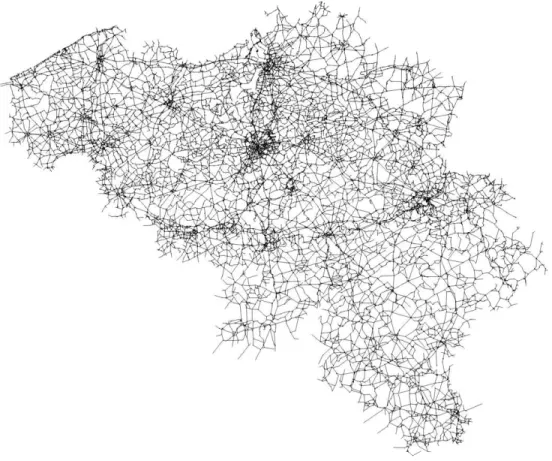
Our activity-based model has been successfully applied to the Belgian synthetic population to simulate an average day. As stated in Section 2, the simulation involved 10,300,000 agents and 4,350,000 households and an average of 4.33 activity per individual i.e. 43.300.000 activities to characterize. The road network considered is illustrated in Figure 4.10, which is made of 66.304 nodes and 125.889 links. It is detailed up to the OpenStreeMap tertiary road network. The sheer size of the simulation generates a substantial amount of computation, whose efficient organization and structuration is truly challenging. The main computational burden is the execution of many shortest-path calculations for activity localization, as well as efficient random draws. After several preliminary attempts, our current best execution time is approximatively 11:00 hours using 500 Intel Xeon X5650 processors’ cores and 1GB of RAM per core, a speed up of a factor 50 on our initial implementation.

Figure 4.10: Belgian road network - 66.304 nodes and 125.889 links

The main output of VirtualBelgium consist of a standard XML file describing the agenda of every agent of the simulation. Listing 1 illustrates the agenda of an agent.

(18)

</person>

Listing 1: An agent’s schedule (XML)

Figure 4.11 show the histogram of proportions of activities starting at each hour of the day. One can easily observe the morning and evening peaks occurring a 8:00 am and 4:00 pm. The comparison of the cumulative distribution functions and the probability density function between the Mobel data and VirtualBelgium is given in Figures 4.12 and 4.13. The Kolmogorov-Smirnov test indicates that these distribution are not significantly different. This result is crucial since it in shows that at an aggregate level, the VirtualBelium agents behave as expected. −5 0 5 10 15 20 25 0 0.01 0.02 0.03 0.04 0.05 0.06 0.07 0.08 0.09 Starting time Proportion

Figure 4.11: Histogram of the number of the number of activity starting at each hour of the day. The difference between VirtualBelgium and Mobel in proportion of activity is presented at Figure 4.14. One can easily see that the differences remains very small, with a mean error of ≃ 0 and a maximum difference less than 10%. This observation seems to validate the generation of activity chain patterns by individual type and the assignment process.

The map illustrated in Figure 4.15 represent the number of activities starting between 8:00 a.m. and 9:00 a.m. by municipalities. As expected, the main cities of Belgium attracts the most part of the activities. This result is encouraging as no indicators were used. This is certainly explained by the fact that these cities have a more dense road network, thus the activity localization process naturally favours them.

As the XML output of VirtualBelgium is compatible with MATSim, it is possible to use it to perform dynamic traffic assignment. For instance Figure 4.16 illustrate a snapshot of the beginning of the morning peak on the Namur city road network. It is nevertheless important to note that every agents use the same transport mode, namely the car, as no mode choice model is currently available in VirtualBelgium.

5 Conclusions and future work

This paper detailed a flexible activity based model implemented in VirtualBelgium, a large agent-based micro-simulation designed to replicate the mobility behaviour of the Belgian population and its evolution. This work demonstrates that assigning and fully characterized (temporally and spatially) a sequence of activities to more than 10.000.000 agents is nowadays feasible.

(19)

−50 0 5 10 15 20 25 0.1 0.2 0.3 0.4 0.5 0.6 0.7 0.8 0.9 1

starting time (hour) Mobel

VirtualBelgium

Figure 4.12: Comparison of the empirical and resulting cumulative distributions.

−50 0 5 10 15 20 25 30 0.01 0.02 0.03 0.04 0.05 0.06 0.07 0.08 0.09

starting time (hour) Mobel

VirtualBelgium

Figure 4.13: Comparison of the empirical and resulting probability density distributions.

The models developed in the VirtualBelgium micro-simulator are data driven and require no a priori informa-tion about the localizainforma-tion of activities. Indeed the minimal requirements are a road network and distribuinforma-tions of the distance and duration for each activity type. Nevertheless the methodology is designed to easily take advantage of any new data sources available such as precise geo-localization of schools and shopping centres, job and services indicators by municipality,... in order to weight or constraints the random draws to specific nodes or municipalities. Moreover the results are promising as the agents mobility behaviour is statistically similar to the ones observed in the Mobel mobility survey. Lastly, the outputs of VirtualBelgium are compatible with MATSim, a powerful and validated micro-simulator for traffic assigment.

Unsurprisingly, the model still requires improvements in order to increase the quality and the reliability of the results. One of the important issue of the current implementation is the lack of a true mode choice for reaching an activity (public transportation, car, walking). In the short term, investigating modal choice ,

(20)

1 2 3 4 5 6 7 8 9 10 11 −0.1 −0.08 −0.06 −0.04 −0.02 0 0.02 0.04 0.06 0.08 purpose difference (proportion) error mean

Figure 4.14: Difference of activity type proportions between VirtualBelgium and Mobel.

less than 2.000 2.000 to 3.500 3.500 tp 5.000 5.000 to 8.000 8.000 to 11.000 11.000 to 16.000 16.000 to 24.000 24.000 to 31.000 31.000 to 60.000 more than 60.000

Figure 4.15: Number of starting activities by municipality between 8:00 am and 9:00 am.

improving data for destination choice (job and service indicators by municipality, schools localization, ...) will also be investigated. Finally, the use of the new tool for estimating OD-matrices is also considered.

Acknowledgements

The authors wish to thanks Frédéric Wautelet and Fran¸cois Damien for their help to set up the simulation on a high performance computing facility. Computational ressources have been provided by the Consortium des Équipements de Calcul Intensif (C ÉCI),

(21)

Figure 4.16: Snapshot of Matsim output. Red agents are stuck in a traffic jam.

funded by the Fonds de la Recherche Scientifique de Belgique (F.R.S.-FNRS) under Grant No. 2.5020.11. Helpful corrections from Eric Cornelis, V´eronique Evrard, Laurie Hollaert and Marie Moriam´e and are also gratefully acknowledged.

References

T. Adler and M. Ben-Akiva. A theoretical and empirical model of trip chaining behavior. Transportation

Research B, 13(3), 477–500, 1979.

T. A. Arentze and H. J. P. Timmermans. Albatross: A learning-based transportation oriented simulation sys-tem. Technical report, European Institute of Retailing and Services Studies. Eindhoven, The Netherlands, 2000.

L. Avery. National Travel Survey: 2010. National Travel Survey. Department for Transport, 2011.

J. Barthelemy and Ph. L. Toint. Synthetic population generation without a sample. Transportation Science, 2012.

C. R. Bhat and F. S. Koppelman. Activity-based modeling of travel demand. in R. W. Hall, ed., ‘Handbook of Transportation Science’, pp. 35–61, Dordrecht, The Netherlands, 1999. Kluwer Academic Publishers. C. R. Bhat, J. Y. Guo, A. Srinivasan, and A. Sivakumar. A Comprehensive Econometric Microsimulator for

Daily Activity-Travel Patterns. Transportation Research Record, 1984, 57–66, 2004.

M. Bradley, J.L. Bowman, and B. Griesenbeck. SACSIM: An applied activity-based model system with fine-level spatial and temporal resolution. Journal of Choice Modelling, 3, 2010.

F.S. Chapin. Human activity patterns in the city: Thing people do in time and space, Vol. 13 of Wiley series

in urban research. J. Wiley and Sons, 1974.

N.T. Collier and M. North. Parallel agent-based simulation with repast for high performance computing.

(22)

E. Cornelis, M. Hubert, Ph. Huynen, K. Lebrun, G. Patriarche, A. De Witte, L. Creemers, K. Declercq, D. Janseens, M. Castaigne, L. Hollaert, and F. Walle. La mobilité en belgique en 2010 : résultats de l’enquête beldam. Technical report, SPF Mobilité et Transports and BELSPO, Brussels, Belgium, 2012. J.W. Dickey. Metropolitan Transportation Planning. McGraw-Hill, New York, USA, 2 edn, 1983.

T. Domencich and D. McFadden. Urban Travel Demand: A Behavioural Analysis. North Holland, Amsterdam, The Netherlands, 1975.

M.L. Eaton. Multivariate statistics: a vector space approach, pp. 116–117. Wiley New York, 1983.

G. Fasano and A. Franceschini. A multidimensional version of the Kolmogorov-Smirnov test. Monthly Notices

of the Royal Astronomical Society, 225, 155–170, 1987.

M.L. Fredman and R.E. Tarjan. Fibonacci heaps and their uses in improved network optimization algorithms.

Journal of the ACM (JACM), 34(3), 596–615, 1987.

L.P. Gan and W. Recker. A mathematical programming formulation of the household activity rescheduling problem. Transportation Research Part B: Methodological, 42(6), 571 – 606, 2008.

T. F. Golob. Structural equation modeling for travel behavior research. Transportation Research Part B:

Methodological, 37(1), 1 – 25, 2003.

J. Goran. Activity based travel demand modelling - a literature study. Technical report, Danmarks Transport-Forskning, 2001.

T. H¨agerstrand. What about people in regional science. Papers of the Regional Science, 4(1), 6–21, 1970. M. M. Haklay and P. Weber. Openstreetmap: User-generated street maps. IEEE Pervasive Computing,

7(4), 12–18, 2008.

S.L. Hoe. Issues and procedures in adopting structural equation modeling technique. Journal of Applied

quantitative methods, 3(1), 76–83, 2008.

J.-P. Hubert and Ph. L. Toint. La mobilit´e quotidienne des Belges. Number 1 in ‘Mobilit´e et Transports’. Presses Universitaires de Namur, Namur, Belgium, 2002.

R. Kitamura, C. Chen, and R. M. Pendyala. Generation of synthetic daily activity-travel patterns.

Transporta-tion Research Record, (1607), 154–162, 1997.

R. Kitamura, E. Pas, C. Lula, T. k. Lawton, and P. Benson. The sequenced activity mobility simulator (SAMS): an integrated approac to modelling transportation, land use and air quality. Transportation, 23, 267–291, 1996.

F. J. Massey. The kolmogorov-smirnov test for goodness of fit. Journal of the American Statistical Association, 46(253), 68–78, 1951.

G. McLachlan and D. Peel. Finite Mixture Models. J. Wiley and Sons, Chichester, England, 2000.

K. Meister, M. Balmer, F. Ciari, A. Horni, M. Rieser, R. A. Waraich, and K.W. Axhausen. Large-scale agent-based travel demand optimization applied to switzerland, including mode choice. paper presented at the 12th World Conference on Transportation Research, July 2010.

E. Miller. Microsimulation and activity-based forecasting. in T. T. Institute, ed., ‘Activity-Based Travel Forecasting Conference: Recommendations, and Compendium of Papers’, pp. 151—-172. Travel Model Improvement Program, US Department of Transportation, US Environmental Protection Agency, June 1996.

K. Nagel, R. L. Beckman, and C. L. Barrett. Transims for transportation planning. in ‘In 6th Int. Conf. on Computers in Urban Planning and Urban Management’. Addison-Wesley, Reading,Massachusetts, 1999. N. Oppenheim. Urban Travel: From Individual Choices to General Equilibrium. J. Wiley and Sons, New York,

(23)

P. Salvini and E. J. Miller. Ilute: An operational prototype of a comprehensive microsimulation model of urban systems. Networks and Spatial Economics, 5, 217–234, 2005.

B.D. Spear. Application of new travel demand forecasting techniques to transportation planning: a study of

individual choice models. Dept. of Transportation, Federal Highway Administration, Office of Highway

Planning, Urban Planning Division, 1977.

K.H. van Dam, I. Nikolic, and Z. Lukszo. based Modelling of Socio-technical Systems, Vol. 9 of

Agent-Based Social Systems Series. Springer-Verlag New York Incorporated, 2012.

P. Waddell. Urbansim: Modeling Urban Development for Land Use, Transportation and Environmental Plan-ning. Journal of the American Planning Association, 3(3), 297–314, 2002.