Are polytopic control design methods suitable for the next robotic control challenges?

HAL Id: tel-02395614

https://hal.archives-ouvertes.fr/tel-02395614

Submitted on 6 Dec 2019

HAL is a multi-disciplinary open access archive for the deposit and dissemination of sci-entific research documents, whether they are pub-lished or not. The documents may come from teaching and research institutions in France or abroad, or from public or private research centers.

L’archive ouverte pluridisciplinaire HAL, est destinée au dépôt et à la diffusion de documents scientifiques de niveau recherche, publiés ou non, émanant des établissements d’enseignement et de recherche français ou étrangers, des laboratoires publics ou privés.

Are polytopic control design methods suitable for the

next robotic control challenges?

Alexandre Kruszewski

To cite this version:

Alexandre Kruszewski. Are polytopic control design methods suitable for the next robotic control challenges?. Automatic. Université de Lille, 2017. �tel-02395614�

Centre de Recherche en Informatique, Signal et Automatique de Lille (CRIStAL) Institut National de Recherche en Informatique et en Automatique (INRIA)

Centrale Lille, Cité Scientifique, CS20048, 59651 Villeneuve-d'Ascq France.

Habilitation à Diriger des Recherches

Génie informatique, automatique et traitement du signal

(Section N°61 du Conseil National des Universités)

Alexandre KRUSZEWSKI

Maître de conférences à Centrale Lille

Docteur en Automatique

Are polytopic control design methods suitable for

the next robotic control challenges?

Soutenue le 12/12/2017 devant le jury suivant:

Président Colot Olivier PR (61) Université de Lille Garant Richard Jean-Pierre PR (61) Centrale Lille

Rapporteur Sala Piqueras Antonio Full Pr. Universitat Polytecnica de Valencia Rapporteur Mounier Hugues PR (61) Université Paris-Sud 11

Rapporteur Poignet Philippe PR (61) Université de Montpellier Membre Brogliato Bernard DR INRIA INRIA Grenoble Rhône-Alpes Membre Duriez Christian DR INRIA INRIA Lille Nord-Europe Membre Guerra Thierry-Marie PR (61) UVHC

2

Summary

Summary ... 2

I. Introduction and Curriculum Vitae ... 3

Curriculum Vitae ... 4

Doctoral co-supervision ... 5

Collaborations and responsibilities ... 5

Personal publications ... 6

II. Polytopic model control design ... 13

Introduction – A control design workflow for polytopic models and its issues ... 13

Output feedback (Maalej 2014; Márquez 2015) ... 21

Conservatism reduction Thesis of Raymundo Márquez (Márquez 2015) ... 30

Conclusions ... 34

References ... 36

III. Networked control system ... 41

Remote control through the Internet ... 41

Bilateral teleoperation through unreliable network ... 49

Other application results ... 59

References ... 60

IV. Perspectives ... 64

Soft robotics control challenges ... 65

Application perspectives: Identify relevant control problems and provide efficient design tools. .. 72

Theory side perspectives: Efficiency, formal computation and Toolboxes. ... 73

Conclusion ... 74

3

I. Introduction and Curriculum Vitae

This manuscript has been written with the aim of passing my Habilitation à Diriger des Recherches (HDR) in the field of control theory. The HDR is a French diploma used to recognize the work of researchers and it allows them to get more autonomy. For example, the HDR is required to be the main supervisor of a PhD student or to apply to a position of Professeur des Universités. I must admit that it is far from being the manuscript I dreamed about. I would have preferred to write something closer to a book with a high tutorial value and enough wisdom to help the readers to choose and use the presented control techniques. Unfortunately, writing such a manuscript is very time consuming and I would not have been able to finish it in a reasonable time (the teaching part of my current position is also very time consuming). This manuscript is not an overview nor a tutorial but it provides the reader with the necessary information to help him in judging the quality of my research. It relates the evolution of my topics, how the different tracks are articulated and the positioning with the respect of the state of the art.

This manuscript is composed with four chapters:

- The first one is dedicated to my curriculum vitae. The information provided in this section is focussed on the research aspect of my productions. There, one finds my complete bibliography, the PhD thesis I co-supervised, my collaborations and my scientific responsibilities.

- The second one deals with my work on the control design by means of polytopic models. The beginning of this section gives an example of use of this technique and tries to depict all sources of conservatism created during the process of getting tractable conditions, i.e. all choices that could result in the loss of potential solutions to the control problem. The second part of this section summarizes a selection of results that I developed with the PhD student I co-supervised which tries to reduce these sources of conservatism.

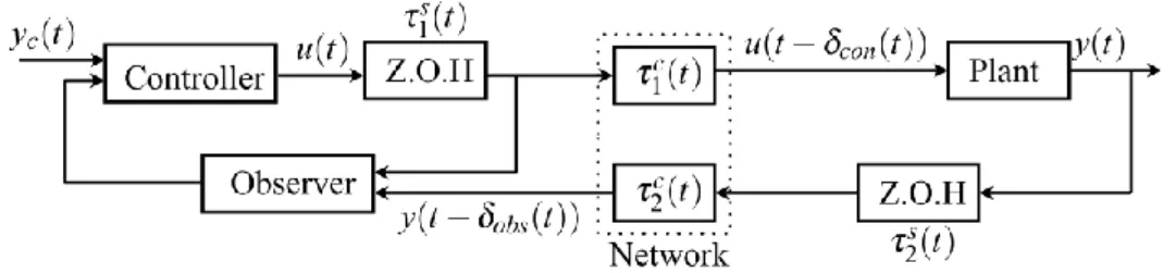
- The third section is application-oriented. It describes the results obtained during two of the PhD supervision I have done in the field of Networked Control System. The first PhD thesis presented deals with the simplest NCS system setup and tries to improve its performances by adapting the control gain according to the Quality Of Service (QoS) of the network. The second PhD thesis is the application of the previously developed techniques on the problem of bilateral teleoperation systems.

- The final section depicts my future research directions which are heavily influenced by a new application topic: the control of deformable robots.

4

Curriculum Vitae

KRUSZEWSKI Alexandre Nationality: French

Date of birth: October 10th, ₁₉₈₁

Place of birth: Dechy (59) France

Position: Maître de conférences (Associate professor) at Centrale Lille since 2007. Member of the DEFROST team (CRIStAL - INRIA).

Laboratories:

CRIStAL1 _{UMR 8022,}

https://www.cristal.univ-lille.fr/ INRIA2 _{Lille – Nord Europe}

https://www.inria.fr/centre/lille Professional address:

Ecole Centrale de Lille

Cité Scientifique, CS20048, 59651 Villeneuve-d'Ascq France. http://www.ec-lille.fr/fr/index.html Tel. +33 3 20 67 60 13 e-mail: alexandre.kruszewski@centralelille.fr Education 2006 PhD thesis

Title: « Lois de commande pour une classe de modèles non linéaires sous la forme Takagi-Sugeno : mise sous forme LMI »

Mention Très Honorable avec Félicitations du Jury:

M. Dambrine Pr Univ. de Valenciennes Jury member

G. Garcia Pr Univ. Toulouse Reviewer

T.-M. Guerra Pr Univ. de Valenciennes Supervisor N. Manamanni Pr Univ. de Reims Champagne-Ardenne Jury member

D. Maquin Pr INPL Nancy Reviewer

J.-P. Richard Pr Ecole Centrale de Lille President A. Sala-Piqueras Pr Univ. Polytecnica Valencia, Spain Jury member

1 _{Centre de Recherche en Informatique, Signal et Automatique de Lille, Villeneuve d’Ascq} 2 _{Institut National de Recherche en Informatique et en Automatique}

5

2004 Master degree: AISIH (Automatique et Informatique des Systèmes Industriels et Humains). Mention Bien, (Major)

2003 Titre d’ingénieur-Maître. Mention Bien (Major)

2002 Licence degree: GEII (Génie électrique et informatique industrielle) 1999 Scientific baccalaureate

Doctoral co-supervision

Defenced co-supervised PhD: 4 Actual PhD co-supervision: 2 2016 – 2019: Thieffry Maxime,

Modélisation et contrôle de robots déformables à grande vitesse, Co-supervisors:

Guerra 20% Duriez 20% Kruszewski 60% 2015 – 2018: Zhang Zhongkai,

New methods of visual servoing for soft-robots,

Co-supervising: Duriez 30%, Dequit 40%, Kruszewski 30% 2011 – 2014: Maalej Sonia,

Commande Robuste des Systèmes à Paramètres Variables,

Co-supervisors: Belkoura 30% Kruszewski 70% 2012 – 2015: Marquez Borbon Raymundo,

Nouveaux schémas de commande et d'observation basés sur les modèles de T-S,

Co-supervisors: Guerra 40% Bernal 20% Kruszewski 40% 2009 – 2012: Zhang Bo,

Commande à retour d'effort à travers des réseaux non dédiés : stabilisation et performance sous retards asymétriques et variables,

Co-supervisors: Richard 50% Kruszewski 50% 2006 – 2009: Jiang Wenjuan,

A contribution to control and observation of networked control systems,

Co-supervisors: Richard 50% Toguyeni 20% Kruszewski 30%

Collaborations and responsibilities

Collaborations:

- ITS, Mexique: M. Bernal (1 PhD co-supervising)

- Université de Valenciennes: T.M. Guerra (2 PhD co-supervising)

- Université de Tel’Aviv, Israël: E. Fridman, (Publications on Network Control System)

- Université de Reims: K. Guelton, N. Manamanni, (Publications on polytopic models

stabilization)

- ENSAM of Lille (L2EP): starting consulting activities on power grid control problems.

Implication in the scientific communities:

- International Program Committee member for:

o IFAC ICONS 2011, 2013, 2015 and 2016

6

o ETFA 2011

- Projects:

o

Member of the European project ‘SYSIASS 6-20' (Autonomous and Intelligent

Healthcare System) [INTERREG IV A 2 Mers Seas Zeen 2007-2013]

o Member of the ANR (Agence Nationale de la Recherche) project ROCC-SYS,

2014-2018

o

Leader of 2 BQR projects (Bonus Qualité Recherche) of Centrale Lille. 10k€

each.

- Expertise:

o

Reviewer of an IDEX (Initiative D’EXellence) project for the Univ. Strasbourg,

2017

o In charge of 4 industrial contracts with the Société Industrielle de Chauffage of

the Atlantic group, since 2012

o Selection committee member of Univ. Valenciennes, 2008-2010

o Recurrent reviewer for Automatica, IEEE TAC, IEEE TFS, Fuzzy sets and

systems, NAHS, …

- Others:

o In charge of some test bench of the SyNeR team (CRIStAL), 2007-2015

o Laboratory council member of CRIStAL, since 2015

Teachings:

- In charge of the coordination of the automatic control teachings at Centrale Lille since

2015

- In charge of 7 modules in automatic control and robotics (linear control, mobile robot

control, robust approaches, LMI, Lyapunov, …) for 3 different engineer formations

- Active participant to the last teaching reform of Centrale Lille

- Teaching charge of ≈240h/year

Other information:

- Change of research team (within CRIStAL) from SyNeR (more theoretical topics) to

DEFROST team (pluridisciplinary team with application to deformable robotics) in

2015.

Personal publications

https://scholar.google.fr/citations?user=4eyt5ewAAAAJ&hl=fr&oi=ao H-index google Scholar total = 14

H-index google Scholar 2012-2016 = 12

Journal papers

[1]

R. Márquez, T. M. Guerra, M. Bernal, and A. Kruszewski, “Asymptotically necessary

and sufficient conditions for Takagi--Sugeno models using generalized non-quadratic

parameter-dependent controller design,” Fuzzy Sets Syst., vol. 306, pp. 48–62, 2017.

7

[2]

S. Maalej, A. Kruszewski, and L. Belkoura, “Robust Control for Continuous LPV

System with Restricted-Model-Based Control,” Circuits, Syst. Signal Process., vol. 36,

no. 6, pp. 2499–25520, 2017.

[3]

S. Maalej, A. Kruszewski, and L. Belkoura, “Stabilization of Takagi–Sugeno models

with non-measured premises: Input-to-state stability approach,” Fuzzy Sets Syst., 2017.

[4]

R. Márquez, T. M. Guerra, M. Bernal, and A. Kruszewski, “A non-quadratic Lyapunov

functional for H8 control of nonlinear systems via Takagi-Sugeno models,” J. Franklin

Inst., vol. 353, no. 4, pp. 781–796, 2016.

[5]

Y.-J. Chen, M. Tanaka, K. Inoue, H. Ohtake, K. Tanaka, T. M. Guerra, A. Kruszewski,

and H. O. Wang, “A nonmonotonically decreasing relaxation approach of Lyapunov

functions to guaranteed cost control for discrete fuzzy systems,” IET Control Theory

Appl., vol. 8, no. 16, pp. 1716–1722, 2014.

[6]

B. Zhang, A. Kruszewski, and J.-P. Richard, “A novel control design for delayed

teleoperation based on delay-scheduled Lyapunov--Krasovskii functionals,” Int. J.

Control, vol. 87, no. 8, pp. 1694–1706, 2014.

[7]

R. Delpoux, L. Hetel, and A. Kruszewski, “Parameter-Dependent Relay Control:

Application to PMSM,” Trans. Control Syst. Technol., vol. 23, no. 4, pp. 1628–1637,

2014.

[8]

R. Marquez, T. M. Guerra, A. Kruszewski, M. Bernal, and others, “Improvements on

Non-Quadratic Stabilization of Takagi-Sugeno Models Via Line-Integral Lyapunov

Functions,” in Intelligent Control and Automation Science, 2013, vol. 3, no. 1, pp. 473–

478.

[9]

K. Guelton, N. Manamanni, A. Kruszewski, T. M. Guerra, and B. Mansouri,

“Commande sous-optimale par retour de sortie pour le suivi de trajectoires des

mod{è}les TS incertains,” J. Eur. des Syst. Autom., vol. 46, no. 4, p. 397, 2012.

[10] A. Kruszewski, W. J. Jiang, E. Fridman, J. P. Richard, and A. Toguyeni, “A switched

system approach to exponential stabilization through communication network,” Control

Syst. Technol. IEEE Trans., vol. 20, no. 4, pp. 887–900, 2012.

[11] A. Kruszewski, R. Bourdais, and W. Perruquetti, “Converging algorithm for a class of

BMI applied on state-dependent stabilization of switched systems,” Nonlinear Anal.

Hybrid Syst., vol. 5, no. 4, pp. 647–654, 2011.

[12] L. Hetel, A. Kruszewski, W. Perruquetti, and J. P. Richard, “Discrete and intersample

analysis of systems with aperiodic sampling,” Autom. Control. IEEE Trans., vol. 56, no.

7, pp. 1696–1701, 2011.

[13] T. M. Guerra, A. Kruszewski, and M. Bernal, “Control law proposition for the

stabilization of discrete Takagi--Sugeno models,” Fuzzy Syst. IEEE Trans., vol. 17, no.

3, pp. 724–731, 2009.

8

[14] T. M. Guerra, A. Kruszewski, and J. Lauber, “Discrete Tagaki--Sugeno models for

control: Where are we?,” Annu. Rev. Control, vol. 33, no. 1, pp. 37–47, 2009.

[15] M. Bernal, T. M. Guerra, and A. Kruszewski, “A membership-function-dependent

approach for stability analysis and controller synthesis of Takagi--Sugeno models,”

Fuzzy sets Syst., vol. 160, no. 19, pp. 2776–2795, 2009.

[16] A. Kruszewski, A. Sala, T. M. Guerra, and C. Ariño, “A triangulation approach to

asymptotically exact conditions for fuzzy summations,” Fuzzy Syst. IEEE Trans., vol.

17, no. 5, pp. 985–994, 2009.

[17] B. Mansouri, N. Manamanni, K. Guelton, A. Kruszewski, and T. M. Guerra, “Output

feedback LMI tracking control conditions with H∞ criterion for uncertain and disturbed

T--S models,” Inf. Sci. (Ny)., vol. 179, no. 4, pp. 446–457, 2009.

[18] F. Delmotte, T. M. Guerra, and A. Kruszewski, “Discrete Takagi--Sugeno’s Fuzzy

Models: Reduction of the Number of LMI in Fuzzy Control Techniques,” Syst. Man,

Cybern. Part B Cybern. IEEE Trans., vol. 38, no. 5, pp. 1423–1427, 2008.

[19] A. Kruszewski, R. Wang, and T. M. Guerra, “Nonquadratic stabilization conditions for

a class of uncertain nonlinear discrete time TS fuzzy models: a new approach,” Autom.

Control. IEEE Trans., vol. 53, no. 2, pp. 606–611, 2008.

[20] T. M. Guerra, A. Kruszewski, L. Vermeiren, and H. Tirmant, “Conditions of output

stabilization for nonlinear models in the Takagi--Sugeno’s form,” Fuzzy Sets Syst., vol.

157, no. 9, pp. 1248–1259, 2006.

[21] H. Tirmant, L. Vermeiren, T. M. Guerra, A. Kruszewski, and M. Parent, “Modélisation

et commande d’un véhicule à deux roues,” J. Eur. des systèmes Autom., vol. 40, no. 4–

5, pp. 535–561, 2006.

International conference papers

[1]

Z. Zhang, J. Dequidt, A. Kruszewski, F. Largilliere, and C. Duriez, “Kinematic modeling

and observer based control of soft robot using real-time Finite Element Method,” in

Intelligent Robots and Systems (IROS), 2016 IEEE/RSJ International Conference on,

2016, pp. 5509–5514.

[2]

R. Márquez, T. M. Guerra, M. Bernal, and A. Kruszewski, “Nested control laws for h8

disturbance rejection based on continuous-time takagi-sugeno models,” in

IFAC-PapersOnLine, 2015, vol. 28, no. 10, pp. 282–287.

[3]

R. Delpoux, L. Hetel, and A. Kruszewski, “Permanent magnet synchronous motor

control via parameter dependent relay control,” in 2014 American Control Conference,

2014, pp. 5230–5235.

[4]

S. Maalej, A. Kruszewski, R. Delpoux, and L. Belkoura, “Derivative based control for

LPV system with unknown parameters: An application on a Permanent Magnet

Synchronous Motors,” in Systems, Signals & Devices (SSD), 2014 11th International

9

[5]

R. Márquez, T. M. Guerra, A. Kruszewski, and M. Bernal, “Non-quadratic stabilization

of second order continuous Takagi-Sugeno descriptor systems via line-integral

Lyapunov function,” in 2014 IEEE International Conference on Fuzzy Systems

(FUZZ-IEEE), 2014, pp. 2451–2456.

[6]

R. Márquez, T. M. Guerra, A. Kruszewski, M. Bernal, and others, “Decoupled nested

LMI conditions for Takagi-Sugeno observer design,” in World Congress, 2014, vol. 47,

no. 1, pp. 7994–7999.

[7]

S. Maalej, A. Kruszewki, and L. Belkoura, “Derivative based control for LTV system

with unknown parameters,” in 2013 European Control Conference, ECC 2013, 2013.

[8]

R. Márquez, T. M. Guerra, A. Kruszewski, and M. Bernal, “Improvements on non-PDC

controller design for Takagi-Sugeno models,” in Fuzzy Systems (FUZZ), 2013 IEEE

International Conference on, 2013, pp. 1–7.

[9]

B. Zhang, A. Kruszewski, J. P. Richard, and others, “H_ {\ infty} Control Design for

Novel Teleoperation System Scheme: A Discrete Approach,” in 10th IFAC Workshop

on Time Delay Systems, 2012.

[10] B. Zhang, A. Kruszewski, J. P. Richard, and others, “H_ {\ infty} Robust Control Design

for Teleoperation Systems,” in 7th IFAC Symposium on Robust Control Design, 2012.

[11] B. Zhang, A. Kruszewski, J. P. Richard, and others, “H_ {\ infty} Control of Delayed

Teleoperation Systems under Polytopic-Type Uncertainties,” in 20th Mediterranean

Conference on Control and Automation, 2012.

[12] B. Zhang, A. Kruszewski, and J. P. Richard, “H∞ control of delayed teleoperation

systems under polytopic-type uncertainties,” in Control & Automation (MED), 2012

20th Mediterranean Conference on, 2012, pp. 954–959.

[13] L. Hetel, A. Kruszewski, W. Perruquetti, and J. P. Richard, “Discrete-time switched

systems, set-theoretic analysis and quasi-quadratic Lyapunov functions,” in Control &

Automation (MED), 2011 19th Mediterranean Conference on, 2011, pp. 1325–1330.

[14] B. Zhang, A. Kruszewski, and J. P. Richard, “A novel control scheme for teleoperation

with guaranteed performance under time-varying delays,” in Control and Decision

Conference (CCDC), 2011 Chinese, 2011, pp. 300–305.

[15] B. Zhang, A. Kruszewski, and J. P. Richard, “Tracking improvement based on the proxy

control scheme for bilateral teleoperation system under time-varying delays,” in

Emerging Technologies & Factory Automation (ETFA), 2011 IEEE 16th Conference on,

2011, pp. 1–8.

[16] W. Jiang, A. Kruszewski, E. Fridman, J. P. Richard, and others, “Delay dependent

stability analysis of interval time-delay systems,” Proc. 9th IFAC Work. Time Delay

10

[17] W. Jiang, A. Kruszewski, J. P. Richard, A. Toguyeni, and others, “A remote observer

and controller with adaptation to the network Quality of Service,” ECC’09, 10th Eur.

Control Conf., EUCA-IFAC-IEEE, 2009.

[18] L. Hetel, A. Kruszewski, T. M. Guerra, and J. P. Richard, “Improved stability conditions

for sampled data systems with jitter,” in Robust Control Design, 2009, vol. 6, no. 1, pp.

273–278.

[19] L. Hetel, A. Kruszewski, and J. P. Richard, “About the Lyapunov exponent of

sampled-data systems with non-uniform sampling,” in Time Delay Systems, 2009, vol. 8, no. 1,

pp. 353–358.

[20] W. Jiang, E. Fridman, A. Kruszewski, and J. P. Richard, “Switching controller for

stabilization of linear systems with switched time-varying delays,” in Decision and

Control, 2009 held jointly with the 2009 28th Chinese Control Conference. CDC/CCC

2009. Proceedings of the 48th IEEE Conference on, 2009, pp. 7923–7928.

[21] R. Bourdais, A. Kruszewski, And W. Perruquetti, “Représentation polytopique pour la

stabilisation des systèmes non linéaires à commutation,” in CIFA, 2008.

[22] A. Kruszewski, T. M. Guerra, and R. Wang, “New approaches for stability and

stabilization analysis of a class of nonlinear discrete time-delay models,” in Fuzzy

Systems, 2008. FUZZ-IEEE 2008.(IEEE World Congress on Computational

Intelligence). IEEE International Conference on, 2008, pp. 402–407.

[23] M. Bernal, T. M. Guerra, and A. Kruszewski, “A membership-function-dependent H∞

controller design for Takagi-Sugeno models,” in Fuzzy Systems, 2008. FUZZ-IEEE

2008.(IEEE World Congress on Computational Intelligence). IEEE International

Conference on, 2008, pp. 1139–1145.

[24] H. Kerkeni, J. Lauber, T. M. Guerra, and A. Kruszewski, “Periodic observer design for

non-linear model with periodic parameters via Takagi-Sugeno form,” in Control and

Automation, 2008 16th Mediterranean Conference on, 2008, pp. 1628–1633.

[25] M. Bernal, T. M. Guerra, and A. Kruszewski, “A membership-function-dependent

stability analysis of Takagi--Sugeno models,” Proc. IFAC World Congr., pp. 5611–

5616, 2008.

[26] W.-J. Jiang, A. Kruszewski, J.-P. Richard, and A. Toguyeni, “A Gain Scheduling

Strategy for the Control and Estimation of a Remote Robot via Internet,” in Proc.

Chinese Control Conference ({CCC}’08), 2008, pp. 793–799.

[27] A. Kruszewski, T. M. Guerra, and M. Bernal, “K-samples variation analysis for

discrete-time Takagi-Sugeno models stabilization: Complexity reduction,” in Advanced Fuzzy

and Neural Control, 2007, vol. 3, no. 1, pp. 37–42.

[28] B. Mansouri, A. Kruszewski, K. Guelton, and N. Manamanni, “Sub-optimal output

tracking control design for uncertain TS models,” in Advanced Fuzzy and Neural

11

[29] T. M. Guerran, M. Bernal, A. Kruszewski, M. Afroun, and L. Vermeiren, “Descripteurs

sous forme T-S : relaxation des résultats en stabilisation,” in LFA’2007, 2007.

[30] A. Kruszewski, A. Sala, T. M. Guerra, and C. Arino, “Sufficient and asymptotic

necessary conditions for the stabilization of Takagi-Sugeno model,” in Advanced Fuzzy

and Neural Control, 2007, vol. 3, no. 1, pp. 55–60.

[31] R. Wang, T. M. Guerra, A. Kruszewski, and J. Pan, “Guaranteed cost control for

uncertain discrete delay TS fuzzy system,” in Advanced Fuzzy and Neural Control, 2007,

vol. 3, no. 1, pp. 85–90.

[32] A. Kruszewski, T. M. Guerra, and S. Labiod, “Stabilization of Takagi-Sugeno discrete

models: towards an unification of the results,” in Fuzzy Systems Conference, 2007.

FUZZ-IEEE 2007. IEEE International, 2007, pp. 1–6.

[33] T. M. Guerra, M. Bernal, A. Kruszewski, and M. Afroun, “A way to improve results for

the stabilization of continuous-time fuzzy descriptor models,” in Decision and Control,

2007 46th IEEE Conference on, 2007, pp. 5960–5964.

[34] W. Renming, T. M. Guerra, A. Kruszewski, And P. A. N. Juntao, “Guaranteed cost

control for uncertain discrete delay TS fuzzy system,” IFAC Proc. Vol., vol. 40, no. 21,

pp. 85–90, 2007.

[35] A. Kruszewski and T. M. Guerra, “Stabilization of a class of nonlinear model with

periodic parameters in the Takagi-Sugeno form,” in Periodic Control Systems, 2007, vol.

3, no. 1, pp. 132–137.

[36] A. Kruszewski, R. Wang, and T. M. Guerra, “New approaches for stabilization of a class

of nonlinear discrete time-delay models,” in Time Delay Systems, 2006, vol. 6, no. 1, pp.

308–313.

[37] A. Kruszewski and T. M. Guerra, “Conditions of output stabilization for uncertain

discrete TS fuzzy models,” 16th IFAC Trienn. World Congr. Prague, Czech Repub.,

2005.

[38] A. Kruszewski, T. M. Guerra, and A. Kruszewski, “New Approaches for the

Stabilization of Discrete Takagi-Sugeno Fuzzy Models,” IEEE Conf. Decis. Control, vol.

44, no. 4, p. 3255, 2005.

[39] T. M. Guerra and A. Kruszewski, “Non-quadratic stabilization conditions for uncertain

discrete nonlinear models in the Takagi-Sugeno’s form,” Work. IFAC AFNC, vol. 4,

2004.

[40]

T. M. Guerra, A. Kruszewski, and J. P. Richard, “Non-quadratic stabilization conditions

for a class of uncertain discrete-time nonlinear models with time-varying delays,” Work.

12

Book Chapters:

[1]

A. Kruszewski, B. Zhang, and J.-P. Richard, “Control Design for Teleoperation over

Unreliable Networks: A Predictor-Based Approach,” in in Delay Systems, Springer

International Publishing, 2014, pp. 87–100.

[2]

W. Jiang, A. Kruszewski, J. P. Richard, A. Toguyeni, and others, “Networked control

and observation for Master-Slave systems,” in in Delay Differential Equations: Recent

Advances and New Directions, Springer, 2009, pp. 31–54.

13

II. Polytopic model control design

Introduction – A control design workflow for polytopic models and its issues

This chapter is dedicated to the presentation of my research results as well as those developed under my supervision by PhD students (Márquez 2015; Maalej 2014). The results presented are dedicated improving the general control design methodology for a class of nonlinear systems. They are focused on the use of polytopic representations of nonlinear models to design a control law. This section focusses on TS (Takagi-Sugeno) (Takagi and Sugeno 1985) models but almost every result also holds for polytopic models in general like the Linear Parameter Varying ones (Briat 2014). The only difference between TS models and other polytopic ones is the background (TS models initially were fuzzy models and most of the results are published in the fuzzy community) and some implicit choices like whether or not to consider the dependency between the state and the scheduling parameters or the rate of variation of the parameter. My references will focus on the TS-related publications.

The TS control framework was successfully used to solve real control and estimation challenges for various application such as bioinspired robotics (Chang, Liou, and Chen 2011), heat exchanger state estimation (Delmotte et al. 2013), wastewater treatment plant parameter estimation (Bezzaoucha et al. 2013), motor cycle lateral dynamic state estimation (Dabladji et al. 2016), spark ignition engine control (Khiar et al. 2007),… I think that TS framework is a valuable tool for the following reasons:

- It allows the engineers to tackle nonlinear control/estimation design by relying on powerful tools coming from the association of Lyapunov theory and demi-definite problem numerical solver in particular Linear Matrix Inequalities solvers (Boyd et al. 1994). - It removes most of the necessary manipulations of complex expressions and most manual

researches of solutions that can be found in nonlinear classical framework. Of course, jumping quickly into numerical analysis has some side effects and one will see that the ease of use is paid by accepting to lose some solutions and mathematical beauty.

I recommend reading the following overviews concerning TS models (T M Guerra, Kruszewski, and Lauber 2009; Thierry M. Guerra, Sala, and Tanaka 2015; Lendek et al. 2011; Sala, Guerra, and Babuška 2005).

To illustrate my research, the rest of this section provides one classical model-based workflow used to find a controller for a nonlinear system using their polytopic representations. At each step, one will highlight my results, the strength and caveats. The last sections of this chapter detail some selected topics.

14

Polytopic-based control design workflow

This subsection presents one of the possible workflows to design a stabilizing controller. For sake of clarity, it will focus only on guaranteeing the stability property of the closed-loop. These results can be extended to performance guarantee by modifying some steps.

Assume that a nonlinear model is available for the control design in the following form:

 

0



 



0



 



1 1 p p j j j j j j

x t

a x

a



z x

x b u

b



z x u

 













(2.1)

 

0



 



0



 



1 1 p p j j j j j j

y t

c x

c



z x

x d u

d



z x u

 













(2.2)

where _{x t }

 

nx _{represents the system state vector, u t }

 

nu _{the input vector,}

y t 

 

ny _the

measured output vector. 𝑎𝑖,𝑏𝑖,𝑐𝑖 and 𝑑𝑖 are matrices with appropriate dimensions.



j

 



, 𝑗 ∈

{1, … , 𝑝} and 𝑧(⋅) are sufficiently smooth nonlinear scalar functions bounded on a compact set of the state space denoted x. Note that the class of models can be extended to the case where 𝑧 is a function

of the state, the input, some parameters or any external signal as long as the functions



j

 

z

 



are

bounded on the sets of interest (generally around an equilibrium point). A quite similar model can be defined in the discrete time domain by replacing 𝑥̇(𝑡) by 𝑥(𝑡 + 1) in (2.1).

Notations:

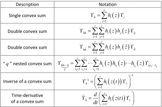
As this chapter deals with polytopic models, one will encounter convex sums expressions. The following shorthand notations will be adopted for sufficiently smooth scalar functions ℎ𝑖 satisfying the convex sum property (∑ ℎ𝑖 𝑖(𝑧) = 1, ℎ𝑖 ≥ 0) and matrices Υi:

Description Notation

Single convex sum

 

1 r h i i i

h z



 





Double convex sum

   

1 1 r r hh i j ij i j h z h z    





Double convex sum ˆ

   

1 1

ˆ

r r i j ij hh i j

h z h z

 

 





“q” nested convex sum ₁

   

₂

 

_{1 2}

1 1 2 1 1 q q h q r r r hh h i i i i i i i i i

h

z h

z

h

z

  





 



Inverse of a convex sum



 



1 1 1 r h i i i h z t       _  _ 



 Time-derivative of a convex sum ₁



( )



r h i i i

d

h z t

dt







 

_



_







15

In the following, one will try to express the conditions as Linear Matrix Inequalities constraints. The following notations will be used to simplify their reading:

- (∗) stands for the smallest expression induced by symmetry.

- “> 0” and “< 0" means respectively positive definite and negative definite when applied to matrix expressions.

Polytopic reformulation

The sector nonlinear approach (Boyd et al. 1994; Tanaka and Wang 2001) is a useful method allowing for an exact polytopic representation of (2.1)-(2.2) over a compact set of the state space x. One just

needs to:

1. Construct the Weighting Functions (WFs) for each nonlinear function



j

 



in the following

form:

 

 

 

 

 

 

 

 

0 , 1 1 0 j j j j j j j z z





z z











         , j



1, 2, ,p



(2.3)

where



_j and



_j are respectively the maximum and the minimum of



j

 



for x  x.

2. Set the membership functions (MFs) as follows:

 

1

 

 

1 2 1 2 2 1 p j p p j i _{i i i} i j j

h

h

_{     } 



z



 

 



, i 



1, 2, , 2p



, i _j

 

0,1 . 3. Obtain the matrices at the polytope vertices:

 

 

_{ 1} i i _h

A

A z

 





,

 

 

_{ } 1 i i _h

B

B z

 





,

 

 

_{ } 1 i i _h

C

C z

 





,

 

 

_{ 1} i i _h

D

D z

 





, i



1, 2, ,r



with

r 

2

p



. Then one gets the following polytopic representation:

 



1 r i i i h h i x h z A x B u A x B u  



  

(2.4)

 



1 r i i i h h i y h z C x D u C x D u  



   . (2.5) where

 

1 1 r i i h   



and h  _i

 

0 and 𝑧 a function of the state and the input. Example:

Let consider the following nonlinear model: 𝑥̇1= cos(𝑥1𝑥2) 𝑥1+ 𝑥2+ 𝑢 𝑥̇2 = sin(𝑥1𝑥2) 𝑥1+ 𝑥2

One can identify two nonlinear functions:



1

 

 

cos x x



1 2



and



2

 

 

sin x x



1 2



. Other choices

16

available for 𝑧(⋅). One can choose for example 𝑧(𝑥) = 𝑥1𝑥2 or,𝑧(𝑥) = 𝑥, of 𝑧(𝑥) = (

cos (𝑥1𝑥2) sin(𝑥1𝑥2)) and so on. For the next step, one chooses 𝑧(𝑥) = 𝑥1𝑥2 and



1

 

 

cos x x



1 2



,



2

 

 

sin x x



1 2



. The

results of the sector nonlinear steps are:

1.

𝜔01(𝑧(⋅)) = 1−cos(𝑥1𝑥2) 2 , 𝜔0 2_{(𝑧(⋅)) =}1−sin(𝑥1𝑥2) 2 , 𝜔1 𝑗 = 1 − 𝜔₀𝑗, 2. ℎ1= 𝜔01𝜔02, ℎ2= 𝜔11𝜔02, ℎ3= 𝜔01𝜔12, 𝑎𝑛𝑑 ℎ1= 𝜔11𝜔12

3. ℎ1= 1 ⇔ 𝜔01= 𝜔02 ⇔ {cos (𝑥1𝑥2) ← 1, sin (𝑥1𝑥2) ← 1 } where ← means ‘subtitute’. The matrices 𝐴𝑖 and 𝐵𝑖 given by:

(cos(𝑥1𝑥2) 𝑥1+ 𝑥2+ 𝑢 sin(𝑥1𝑥2) 𝑥1+ 𝑥2 )|𝜁1=𝜁̲2 𝜁_2=𝜁̲2 = [1 1 1 1] ⏟ 𝐴1 𝑥 + [1 0] ⏟ 𝐵1 𝑢 (cos(𝑥1𝑥2) 𝑥1+ 𝑥2+ 𝑢 sin(𝑥1𝑥2) 𝑥1+ 𝑥2 )|𝜁1=𝜁̅2 𝜁_2=𝜁̲2 = [−1 1 1 1] ⏟ 𝐴2 𝑥 + [1 0] ⏟ 𝐵2 𝑢 …

The reader may refer to (Márquez 2015; A Kruszewski 2006; Tanaka and Wang 2001) for more details. It is important to note that, because this transformation is not unique, it may impact the control design result and conservatism3_{. The only known result trying to optimize this choice is reported in (Robles et}

al. 2016).

Choose a control structure

Once the model has been redefined in a polytopic form one has to choose the right control structure. Being exhaustive would not help at all. One will focus on the classical tools for control: state feedback and state observer when necessary.

It can be proven that for quadratic stabilization in the continuous case, it is necessary and sufficient to consider a PDC control law (parallel distributed compensation) to stabilize a TS system. If one does not care about reference tracking, these control laws can be reduced to the following expression:

𝑢(𝑡) = −𝐹ℎ𝑥(𝑡). (2.6)

Despite this property, some results managed to get less conservative results using more complex control laws (Márquez et al. 2013; Márquez et al. 2015a; Márquez et al. 2015b; Márquez et al. 2017). These results are the topic of another subsection of this chapter and explains this strange result. When it comes to the output feedback problem, the natural way is to consider the use of state observer which use the same structure as the model:

 









ˆ ˆ ˆ





1

ˆ

r _i

ˆ

_i

ˆ

_{i i}

ˆ

ˆ

ˆ

h h h i

x

h z

A x

B u

K y

y

A x

B u

K

y

y





















(2.7)

 



ˆ ˆ 1

ˆ

r _i

ˆ

_i

ˆ

_i h h i

y

h z C x

D u

C x

D u













. (2.8)

17

This observer structure allows to reuse a state feedback control law 𝑢(𝑡) = −𝐹_ℎ̂𝑥̂(𝑡). From here, one must study two cases: the case where the arguments of the nonlinear functions are measured (𝑧̂ = 𝑧) and the case they are not (𝑧̂ ≠ 𝑧). The first case is quite nice since the separation principle applies and both problems (observation and control) can be studied separately (Tanaka and Wang 2001). The second one is still an open problem and often reduces the global stability property to local stability property. Some results about this topic and alternative possibilities are discussed later in this manuscript (Maalej, Kruszewski, and Belkoura 2017b; Thierry Marie Guerra et al. 2017; Maalej 2014; Márquez 2015).

Choose a Lyapunov function

For this class of model, it is convenient to use the direct Lyapunov method to deal with stability. An important choice is the formulation of the Lyapunov function (LF). Many papers consider the problem of finding a quadratic Lyapunov function, i.e.:

𝐹𝑖𝑛𝑑 𝑃 ∈ ℝ𝑛×𝑛 𝑠. 𝑡. 𝑉(𝑥) = 𝑥𝑇𝑃𝑥 > 0 ∀𝑥 ≠ 0

𝑑

𝑑𝑡𝑉(𝑥(𝑡)) < 0 ∀𝑥(𝑡) ≠ 0 along the trajectories of the system (2.7)

This choice is not suitable for all polytopic model and is quite conservative4_{. Many attempts were made}

to leave this class of LF and tried to use nonquadratic function (NQLF).

One should distinguish the continuous case from the discrete case ((2.4) with 𝑥(𝑡 + 1) instead of 𝑥̇(𝑡) and 𝑉(𝑥(𝑡 + 1)) − 𝑉(𝑥(𝑡)) < 0 instead of 𝑉̇ < 0). The discrete case is the easiest one. By considering nonquadratic LF like 𝑉(𝑥) = 𝑥𝑇𝑃ℎ𝑥 or non-monotically decreasing LF 𝑉(𝑥(𝑡 + 𝑘)) − 𝑉(𝑥(𝑡)) < 0 with 𝑘 ≥ 2 leads to good relaxation of the results. Based on the later results one also find the Asymptotically Necessary and Sufficient (ANS) class of Lyapunov function (Hetel et al. 2011) and ANS LMI conditions (A Kruszewski and Guerra 2007b; A Kruszewski, Guerra, and Kruszewski 2005; A Kruszewski and Guerra 2005; Chen et al. 2014; T M Guerra and Kruszewski 2004; T M Guerra, Kruszewski, and Bernal 2009; A Kruszewski, Guerra, and Bernal 2007; T M Guerra, Kruszewski, and Lauber 2009; T M Guerra and Kruszewski 2005; A Kruszewski and Guerra 2007a; Alexandre Kruszewski, Guerra, and WANG 2008; A Kruszewski, Wang, and Guerra 2008) for this class of polytopic model (when ignoring the shape of the functions ℎ𝑖). (Hetel et al. 2011) proposed a link between this approach and an equivalent LF with 𝑘 = 1. Despite the ANS property, there is a lot a room for improvement to reduce the complexity of the condition and to make these results numerically tractable.

In the continuous-time case, the main problem comes from the introduction of the time derivative of the nonlinear parts of the LF while trying to ensure 𝑉̇ < 0. For example, if one chooses the candidate:

𝑉(𝑥) = 𝑥𝑇𝑃ℎ𝑥 = 𝑥 ∑𝑟𝑖=1ℎ𝑖(𝑧(⋅))𝑃𝑖𝑥 The variation of the LF along 𝑥(𝑡) becomes:

𝑉̇(𝑥) = 𝑥𝑇𝑃ℎ𝑥̇ + 𝑥̇𝑇𝑃ℎ𝑥 + 𝑥𝑇𝑃̇ℎ𝑥 = 𝑥𝑇𝑃ℎ𝑥̇ + 𝑥̇𝑇𝑃ℎ𝑥 + 𝑥𝑇∑ 𝑑 𝑑𝑡ℎ𝑖(𝑧(∙))𝑃𝑖 𝑟 𝑖=1 𝑥

18

In this expression, the two first terms are easily handled as in the quadratic case. The last term is not signed and needs to be bounded. The use of these bounds reduces the stability proof to a local region of the state space. Two kinds of assumption are used in this case:

- Consider |ℎ̇𝑖| < ϕi (Tanaka and Wang 2001; Mozelli, Palhares, and Avellar 2009) which is problematic in control design due to the link between the bounds ϕi and the control law, i.e.:

ℎ̇𝑖 = 𝑑 𝑑𝑡ℎ (𝑧(𝑥(𝑡))) = 𝜕ℎ(𝑧(𝑥)) 𝜕𝑥 𝑑𝑥 𝑑𝑡 = 𝜕ℎ(𝑧(𝑥)) 𝜕𝑥 (𝐴𝑥 + 𝐵𝑢)

In that case, the invariant set depends on the control law and can only be computed a posteriori. It is difficult in this case to optimize the invariant set of the closed loop.

- Consider a bound on the partial derivatives which helps in mastering the invariant set (Pan et al. 2012; T.-M. Guerra and Bernal 2009; Sala et al. 2010) by writing something like:

   



1 2



0 , , 1 1 k p r i g i k g i k k h i k k

P

h

P

P

z

z



 











… 0 k l kl k

x

z



_







where 𝜔𝑖 are the constitutives elements of the ℎ𝑖.

Remark: Knowing that the use of NQLF extends the possibilities in stabilization, it is not sure that all the control law designed with such LF are still robust as we may be considering a limit case. That is why I think it is preferable to introduce some robustness guarantee when nonquadratic LF are used (in the form of artificial parameter uncertainty or a state disturbance for example).

LMI formulation

Once a LF has been selected, it is convenient to reformulate the stability/stabilization conditions as a set of Linear Matrix Inequalities (LMI). LMI formulation is the backbone of the polytopic approach as it provide an effective way to numerically solve the conditions (global convergence, feasibility check and polynomial time computation) (Boyd et al. 1994; Gahinet et al., n.d.).

For example, in continuous time (2.4) with a PDC control law (2.6) if there exist matrices 𝑃 = 𝑃𝑇 such that:

𝑉(𝑥) = 𝑥𝑇_{𝑃𝑥 > 0 ∀𝑥 ≠ 0}

𝑉̇(𝑥(𝑡)) = 𝑥𝑇_{𝑃𝑥̇ + 𝑥̇}𝑇_{𝑃𝑥 = 𝑥}𝑇_𝑃(𝐴

ℎ− 𝐵ℎ𝐹ℎ)𝑥 + (∗) < 0 ∀𝑥 ≠ 0

then the closed loop is stable. This stability criterion is equivalent to the following matrix inequality conditions:

{_𝑃(𝐴 𝑃 > 0

ℎ− 𝐵ℎ𝐹ℎ) + (∗) < 0 (2.9)

Where “> 0” and “< 0" means respectively positive definite and negative definite. These conditions are not linear in the decision variables (the entries of 𝑃 and the 𝐹𝑖 enclosed in 𝐹ℎ)

Linearization of the stabilization problem:

Multiple properties are available which help to get LMI conditions. They can be classified in three groups:

- Necessary and sufficient properties:

In this group we can find useful lemma and matrix transformations which do not introduce conservatism. The first transformations one should know are: the bijective changes of variables (like 𝑌 = 𝐹𝑋 where 𝑋 is an invertible matrix) and the congruence (left multiplication with a full rank matrix and right multiplication with its transpose). Other useful lemmas exist and helps in getting a LMI problem formulation: the Schur complement lemma which helps

19

removing some quadratic terms, the Finsler lemma and the S-procedure to check a condition under state restrictions. These manipulations can be found in (Boyd et al. 1994)

- Bounding methods:

This group consists in all other tools that should be used when no other options are available. They consist in approximating (find a guaranteed bound) non-convex term with linear ones. For example, the matrix square completion 𝑋𝑇𝑌 + 𝑌𝑇𝑋 ≤ 𝑋𝑇𝑋 + 𝑌𝑇𝑌 and all its variations, Jensen inequality to deal with integral terms (Gu, Chen, and Kharitonov 2003), Finsler lemma with restrictions on slack matrices, and so on…

- LMI sequence algorithms:

It consists in a loop of LMI problems of solve in which one solves the optimization problem for different set of decision variable. For example: if one wants to find a solution to: {

find 𝑃, 𝐹 s. t. : 𝑃𝐴 + 𝑃𝐵𝐹 + (∗) < 0

𝑃 = 𝑃𝑇 _{> 0} Then one can try:

o Initialize 𝑃0= 𝐼 and 𝑘 = 0 o Do:  𝑘 = 𝑘 + 1  Solve { find 𝐹𝑘, maximize 𝑡 s. t. : 𝑃𝑘−1𝐴 + 𝑃𝑘−1𝐵𝐹𝑘+ (∗) < −𝑡 𝑃𝑘−1= 𝑃𝑘−1𝑇 > 𝑡  Solve { find 𝑃𝑘, maximize 𝑡 s. t. : 𝑃𝑘𝐴 + 𝑃𝑘𝐵𝐹𝑘+ (∗) < −𝑡 𝑃𝑘 = 𝑃𝑘𝑇 > 𝑡 o Until {𝑃𝑘𝐴 + 𝑃𝑘𝐵𝐹𝑘+ (∗) < 0 𝑃𝑘 = 𝑃𝑘𝑇> 0

These linearization techniques are presented in order of preference: - the first one is exact and no solution are lost,

- the last one is the worst as it depends on the initialization of the algorithm, the choice of the decision variable sets (when multiple solutions are available) as well as the optimization criteria that is used.

If one wants to apply such techniques on the classical stabilization problem one should apply the congruence with 𝑃−1 on (2.9):

{ 𝑃−1> 0

𝐴ℎ𝑃−1− 𝐵ℎ𝐹ℎ𝑃−1+ (∗) < 0 (2.10)

Using bijective transformations 𝑋 = 𝑃−1 and 𝑌𝑖 = 𝐹𝑖𝑃−1 the stabilization problem (2.9) becomes: { 𝑓𝑖𝑛𝑑 𝑋 = 𝑋𝑇 _{𝑎𝑛𝑑 𝐹} 𝑖 𝑠. 𝑡. 𝑋 > 0 𝐴ℎ𝑋 − 𝐵ℎ𝑌ℎ+ (∗) < 0 (2.11)

Or by exposing the convex sums:

{ 𝑓𝑖𝑛𝑑 𝑋 = 𝑋𝑇 𝑎𝑛𝑑 𝐹𝑖 𝑠. 𝑡. ∀ℎ𝑖(⋅) ∈ [0 1], ∑𝑟𝑖=1ℎ𝑖(⋅)= 1 𝑋 > 0 ∑𝑖=1𝑟 ∑𝑟𝑗=1ℎ𝑖(⋅)ℎ𝑗(⋅) (𝐴𝑖𝑋 − 𝐵𝑖𝑌𝑗+ (∗))< 0 (2.12)

20

The optimization problem (2.12) is linear according to the decision variable but cannot be solve yet. It represents an infinite number of LMI constraint due to the dependence on the functions ℎ𝑖.

Convex embedding

Convex embedding corresponds to the techniques transforming an infinite set of LMI into a finite one, more suitable for numerical solving. Most of the time it consists in transforming a multiple sum problem like (2.11):

{_𝐴 𝑋 > 0

ℎ𝑋 − 𝐵ℎ𝑌ℎ+ (∗) < 0 ⇔ {

𝑋 > 0

∑ ∑ ℎ𝑖 𝑗 _𝑖(𝑧)ℎ_𝑗(𝑧) (𝐴_𝑖𝑋 − 𝐵𝑖𝑌𝑗+ (∗))< 0 (2.13) Unfortunately, all results available to deal with this transformation are conservative. The roughest result is to simply consider that each term of the sum is negative definite:

𝐴𝑖𝑋 − 𝐵𝑖𝑌𝑗+ (∗) < 0 ∀𝑖, 𝑗

This is problematic because one can prove that these inequalities have solutions only if a linear state feedback is available (each the gain 𝐹𝑗 stabilizes all the linear models (𝐴𝑖, 𝐵𝑖)).

Several techniques are available in the literature (Kim and Lee 2000; Tuan et al. 2001; Sala and Ariño 2007; A Kruszewski et al. 2007; A Kruszewski et al. 2009) introducing more or less complexity to the numerical problem (number of decision variable and combined size of the problem). One should note the results of (Ario and Sala 2008; A Kruszewski et al. 2007; A Kruszewski et al. 2009) provide Asymptotically Necessary and Sufficient (ANCS) conditions. They allow to choose the accuracy/complexity ratio of the convex embedding with a proof of convergence to the infinite size problem (2.12). Unfortunately, the computational complexity is exponential and the ratio parameter must stay quite low to be numerically tractable. The results of (Tuan et al. 2001) are also interesting and I think they are the most efficient result for the moment, and should be tried first.

The conditions of (Tuan et al. 2001) are the following:









_{ }

1 1 2 1

0

0,

1, 2,

,

2

0,

( , )

1, 2,

,

,

.

0,1

1

1

r r i j ij ii i i r ii ij ji i i i

h h

i

r

i j

r

i

j

h

h

r

  



_{ }

 

 



_



_







     









_{ }

_

 

_





Applying this lemma with

 

ij

A X

i



B F

i j makes (2.12) a LMI problem with a finite set of constraints.

One can see here that the conditions lose some knowledge about the functions ℎ𝑖 as the conditions ensure (2.12) for any functions ℎ𝑖 with satisfying the convex sum property.

Only few results exploit the shape of the weighting function or optimize the choice of the ℎ𝑖 during the sector nonlinear approach which potentially reduces a lot the conservatism (Bernal, Guerra, and Kruszewski 2009; Robles et al. 2016; Bernal, Guerra, and Kruszewski 2008a; Bernal, Guerra, and Kruszewski 2008b). Most of the available results only rely on the convex sum property of the weighting functions ℎ𝑖 which is quite problematic because all the knowledge of the nonlinear function is lost and impossible situations may be considered unnecessarily (like cos(𝑥1𝑥2) = 1 and sin(𝑥1𝑥2) = 1 at the same time).

21

Get a solution

Solvers are available for this kind of convex optimization problem (Sturm 1999; Gahinet et al., n.d.; Löfberg 2004). When there are no numerical problems, they provide the global optimal solution if any and can state the unfeasibility of the conditions. Getting a solution is easy if the problem is not too large (size of the LMI problem + number of decision variable) or if not ill-conditioned.

When it fails

If the solver fails in finding a consistent solution (feasible solution + realistic control gains) because of the complexity or the nonlinear nature of the problem, some backup options are available:

- Rewrite the problem by splitting it in small pieces, study them separately and use for example Input-to-state gains (Sontag 2008) to glue them back together. This approach is conservative because it relies on the ISS small gain theorem but helps in exploring new solutions (for example see (Maalej, Kruszewski, and Belkoura 2017b)).

- Try to approximate the model to find control gains then check the stability on the former one. This helps in reducing the number of decision variables. However, the sequential implementation (find the gains, then find the LF) introduces conservatism.

- Try to apply redesign techniques, for example: design a linear state feedback with pole placement techniques and then convert back the solution to the former problem (Delpoux, Hetel, and Kruszewski 2014).

- Avoid completely the numerical resolution of the LMI problem. For example use a more generic control strategy (Maalej 2014).

This workflow proposition was restricted to stabilization. If one wants to deal with performances, one must change the model definition and the starting condition (𝑉̇ < 0). Problems may appear in the linearization step where the introduction of performances may certainly introduce nonlinear terms. Due to the conservative nature of this workflow, the performances can only be guaranteed above the specified level. The real performances being always better than what was predicted/required (for some case, the difference is huge).

The next two sections provide some details about the works I supervised. These results comes from two PhD thesis (Maalej 2014; Márquez 2015). The first section focuses on output feedback solutions in the case where the premise vector 𝑧(⋅) is not measured. It proposes three solutions based on different control strategies (used of TS observer, linear observer or derivative estimator). The second one deals with the conservatism reduction of state-feedback stabilization conditions and present the results obtained with different Lyapunov functions.

My works on polytopic approaches are not limited to this perimeter and also includes results on tracking, performances, discrete time, descriptor, … (see the bibliography section).

Output feedback (Maalej 2014; Márquez 2015)

This section provides additional details about the problem of observer-based output feedback for TS models. It focusses on the hard case where the premises variables are not available.

Let us consider the following polytopic representation of the system:

 



1 r i i i h h i x h z A x B u A x B u  



  

(2.14)

 



1 r i i i h h i y h z C x D u C x D u  



   . (2.15)

22

and the standard observer for this class of polytopic models (Tanaka and Wang 2001):

 









ˆ ˆ ˆ





1

ˆ

r _i

ˆ

_i

ˆ

_{i i}

ˆ

ˆ

ˆ

h h h i

x

h z

A x

B u

K y

y

A x

B u

K

y

y





















(2.16)

 



ˆ ˆ 1

ˆ

r _i

ˆ

_i

ˆ

_i h h i

y

h z C x

D u

C x

D u













. (2.17)

The observation error system writes:





ˆˆ ˆ ˆ ˆˆ h h h h h h h eA xA xB uB uK C x C x or



_hˆ _hˆ

 

h _hˆ

 

h _hˆ



_hˆ



h _hˆ



e



A



K C e



A



A x



B



B u



K

C



C

x

(2.18) Separation principle applies when 𝑧̂ = 𝑧 as one can write the following error model:



h h h



e



A



K C

e

(2.19)

The evolution of (2.19) is completely independent from the one of (2.14). The closed loop (2.14) with a PDC u F x_hˆˆ F xh F eh becomes:

h h h h h

xA xB F xB F e (2.20)

Then by the input to state properties (Sontag 2008) one can state that if (2.20) is stable for 𝑒 = 0 and if 𝑒 is 𝐿2 bounded then (2.20) is stable. It proves that if the solutions of the error model (2.19) converge and if 𝑥̇ = 𝐴ℎ𝑥 − 𝐵ℎ𝐹ℎ is stable then closed loop is be stable.

The case where 𝑧 = 𝑧̂ is reductive since it means that not only the output has to be measured but also the argument of the membership function. For the case 𝑧̂ ≠ 𝑧, the theory is more complicated and further investigation must be done: one cannot separate the two stability problems and it leads to non-convex optimization problems when one is searching for the LF matrices 𝑃𝑒 and 𝑃𝑥 , the control gains 𝐹𝑖 and observation gains 𝐾𝑖.

Some results from the literature propose solutions to this problem. The first one (T M Guerra et al. 2006) proposes a really rough manner to deal with the problem and is very conservative. This conservativeness comes from the fact that no connections are made between the functions ℎ𝑖 and the functions ℎ̂𝑖. To overcome this limitation, one need to consider additional assumptions like the knowledge of a Lipchitz constant of the functions ℎ𝑖 (D. Ichalal et al. 2010; Dalil Ichalal et al. 2010; P Bergsten and Palm 2000).

The next subsections present some results of thesis I co-supervised. The first one is related to the thesis (Márquez 2015) and provides new conditions for convergence of state observer in the case of non-measured premises. The second and the third ones are related to another thesis I co-supervised (Maalej 2014) in which one proposes to consider the problem of output feedback as an interconnection of two sub-systems. Then by using input-to-state properties one can derive conditions which does not depends on extra assumption of the membership functions. The last result proposed is to change the output feedback structure but the results only guarantee the stability and performances for a specific class of system. The resulting controller requires the knowledge of only three model parameters to be tuned.

23

Using the differential mean value theorem (Thierry Marie Guerra et al. 2017)

The paper (Thierry Marie Guerra et al. 2017) provides a result that was developed during the thesis of (Márquez 2015) that I have co-supervised. It presents a solution for observer design in the case of non-measured premises observers. This solution is based on the differential mean value theorem which helps in characterising the evolution of ℎ𝑖(𝑧(𝑡)) − ℎ𝑖(𝑧̂(𝑡)). The resulting conditions ensure the observation error convergence as well as 𝐿2→ 𝐿2 gain performances.

To illustrate this result, let us consider the following observer:

 













 

ˆ ˆ ˆ 1 ˆ 1 ˆ ˆ ˆ ˆ ˆ ˆ ˆ ˆ ˆ. r i i i i h h h i r i i h i x h z A x B u K y y A x B u K y y y h z C x C x            





To reduce the conservatism, one considers the separation

h

ˆ





ˆ

between what is measured 𝛼(𝑧(⋅)) ≜ 𝛼 in the ℎ̂ function and what is not 𝛽(𝑧̂(⋅)) ≜ 𝛽̂. This decomposition is performed during the polytopic reformulation of the model by applying the sector nonlinear approach twice: on the measured part, then on the non-measured part of the nonlinearities.

With this decomposition, the nonmatched terms in the observation error equations (2.18) become:

 



 

 



 



 

 



 



 

 



ˆ ˆ 1 1 ˆ ˆ 1 1 ˆ ˆ 1 1 ˆ , ˆ , ˆ . r r h h i j j ij i j r r h h i j j ij i j r r h _h i j j ij i j A A A A z z z A B B B B z z z B C C C C z z z C                  _   



















               _{    }     _{    } 







(2.21)

Then, after applying the differential mean value theorem, one writes:

 

 

 

 

 

ˆ 1 1 1 ˆ 1 ˆ 1

,

,

r r r i j z ij j z j i j j r j z j j r j z j j

A

A

z

c e A

c e A

B

B

c e B

C

C

c e C

              











    



















_

_

_









_

_

_











(2.22) with j

 

j

 

z c z c z





     and ez z zˆ.

For sake of conciseness, the technical developments towards the LMI formulation are omitted. The important fact is that one assume that the partial derivative of the non-measured membership functions 𝜕𝛽𝑗(𝑧)

𝜕𝑧 are bounded as well as the state 𝑥(𝑡) and the control input 𝑢(𝑡), i.e:. ‖ 𝜕𝛽𝑗(𝑧)

𝜕𝑧 ‖ ≤ 𝜎𝑗, ‖𝑥‖ ≤ 𝜆𝑥 and ‖𝑢‖ ≤ 𝜆𝑢

24

In order to illustrate the efficiency of this approach, let us consider the following nonlinear plant:









1 2 1 2 1 2 1 2 1 3 0 4 3 1 4 a x x b x x u x x x x x y x  _{ }   _{    }  _{    }      _{ }      

with the model validity set x 



x x: 1x2 4



. Fig 2.1 shows the feasibility set of the LMI

conditions if the space (𝑎, 𝑏) of (Thierry Marie Guerra et al. 2017) compared to the Lipchitz based of (Dalil Ichalal et al. 2007) and (Pontus Bergsten, Palm, and Driankov 2001). The new conditions are able to find more solutions than older ones.

Fig 2.1 Feasibility region: “ ” for conditions is (Thierry Marie Guerra et al. 2017), “” for conditions in (Dalil Ichalal et al. 2007), and “” for conditions in (Pontus Bergsten,

Palm, and Driankov 2001)

An extension with 𝐿2→ 𝐿2 attenuation (noise 𝑤 to estimation error 𝑒) is also provided in of (Thierry Marie Guerra et al. 2017) and the numerical results are compared with (Dalil Ichalal et al. 2011) which is also based on the mean value theorem. The comparison is performed on the following plant:

 

 

 

 

 





2 1 2 2 2

0.1 0.1

1.5 0.5

1.5

1.5

0

,

1

0.1

2

4

1

1 10

1 0

,

x

x

a

x

x

x

u

w

x

x

y

x





























 

_

_



_

_



_{ }



_

_





 

_{ }





_

_

_







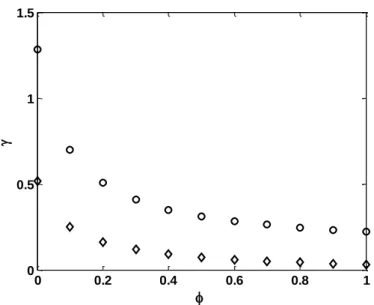
Fig 2.2 shows the guaranteed 𝐿2→ 𝐿2 attenuation obtained for different values of the parameter 𝜙.

-2 -1.5 -1 -0.5 0 0.5 1 1.5 2 -2 -1.5 -1 -0.5 0 0.5 1 1.5 2 2.5 3 Parameter "a" Parame ter " b"