HAL Id: tel-02047005
https://hal.sorbonne-universite.fr/tel-02047005
Submitted on 23 Feb 2019
HAL is a multi-disciplinary open access archive for the deposit and dissemination of sci-entific research documents, whether they are pub-lished or not. The documents may come from teaching and research institutions in France or
L’archive ouverte pluridisciplinaire HAL, est destinée au dépôt et à la diffusion de documents scientifiques de niveau recherche, publiés ou non, émanant des établissements d’enseignement et de recherche français ou étrangers, des laboratoires
architectured materials
Justin Dirrenberger
To cite this version:
Justin Dirrenberger. Towards an integrated approach for the development of architectured materials. Engineering Sciences [physics]. Sorbonne Université, 2018. �tel-02047005�
H
D
R
UFR 919 - IngénierieMémoire d’habilitation
en vue de l’obtention de l’habilitation à diriger des recherches
présenté et soutenu publiquement par
Justin DIRRENBERGER
le 18 décembre 2018Vers une approche intégrée pour le développement des
matériaux architecturés
Towards an integrated approach for the development of
architectured materials
Jury
Véronique AUBIN,Professeur, CentraleSupélec Rapporteur
Jean-François CARON,Directeur de recherche, ENPC Rapporteur
Damien FABREGUE,Professeur, INSA Lyon Rapporteur
Jean-Pierre CHEVALIER,Professeur, CNAM Examinateur
Hélène DUMONTET,Professeur, Sorbonne Université Examinateur
Contents
List of notations iii
I Introduction 1 0 Introduction 3 0.1 Introduction . . . 3 0.2 A personal brief. . . 4 0.3 Outline. . . 4 II Scientific overview 7 1 Microstructural representativity 9 1.1 Representative volume element . . . 10
1.1.1 RVE size determination for media with finite integral range . . . 12
1.1.2 Generalisation of the statistical approach to microstructures with non-finite integral range . . . 14
1.2 Evaluation of morphological representative sample sizes for nanolayered polymer blends . . . 16
1.2.1 Materials and characterisation techniques . . . 17
1.2.2 Representativity of AFM samples . . . 21
1.2.3 Results and discussion . . . 23
1.2.4 Conclusions and perspectives . . . 28
1.3 RVE size determination for viscoplastic properties in polycrystalline materials. . 29
1.3.1 Introduction . . . 29
1.3.2 Crystal plasticity constitutive model . . . 31
1.3.3 Computational approach . . . 31
1.3.4 Results and discussion . . . 35
1.3.5 Conclusions and perspectives . . . 40
1.4 Outlook . . . 41
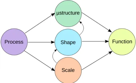
2 Architectured materials 43 2.1 Introduction to architectured materials . . . 43
2.2 Computational homogenisation of architectured materials. . . 48
2.2.1 Constitutive equations . . . 48
2.2.2 Averaging relations . . . 50
2.2.3 Boundary conditions . . . 51
2.2.4 Hill–Mandel condition . . . 52
2.2.5 Effective properties vs. apparent properties . . . 52
2.2.6 Computational homogenisation using the finite element method . . . 55
2.2.7 Conclusions . . . 58
2.3 Architectured auxetic hybrid lattice structures . . . 58
2.3.1 Lattice structures . . . 58
2.3.2 Additively manufactured lattice structures . . . 61
2.3.3 Materials and methods . . . 62
2.3.4 Microstructural and mechanical characterisation . . . 63
2.3.5 Simulation and computational homogenisation . . . 63
2.4 Control of instabilities through architecture . . . 65
2.5 Modelling architectured materials with generalised continua . . . 68
2.6 Shape optimisation for additive manufacturing . . . 70
2.6.1 Smoothed and manufacturable hinge-type vertices . . . 71
2.6.2 Computational strategy . . . 72
2.6.3 Results . . . 73
2.6.4 Conclusions . . . 76
2.7 Localised laser processing for metal sheets . . . 77
3 Scaling up 83 3.1 Computation for design, modelling, and manufacturing . . . 83
3.2 Towards large-scale additive manufacturing. . . 86
3.3 Creating a technology company. . . 89
3.3.1 A new playground for multidisciplinary research . . . 90
3.3.2 Concrete formwork 3D printing . . . 91
3.3.3 Case study: Post in Aix-en-Provence, France . . . 91
3.4 Masonry 4.0. . . 99
III Future work 103 4 General conclusions and proposal for future work 105 4.1 General conclusions . . . 105
4.2 Mechanical behaviour of architectured materials . . . 106
4.3 Hierarchical morphologies . . . 106
References 109
Curriculum Vitæ 151
Scientific output 153
List of Notations
Tensors, tensor algebra and operators
x 0th-order tensor (scalar)
x orxi 1st-order tensor (vector)
x∼ orxi j 2nd-order tensor x ≈ orxi j kl 4 th-order tensor I ∼ orIi j 2
nd-order identity tensor
I
≈ orIi j kl 4
th-order identity tensor
x = a · b x = aibi x = a∼· b xi= ai jbj x∼= a∼· b∼ xi j= ai kbk j x = a∼: b∼ x = ai jbi j x∼= a≈: b∼ xi j= ai j klbkl x = a≈:: b ≈ x = ai j klbi j kl x∼= a ⊗ b xi j= ajbj x∼= a ⊗ b =s 12³a ⊗ b + ¡a ⊗ b ¢T´ x(i j )=1 2 ¡ aibj+ ajbi¢ x≈= a∼⊗ b∼ xi j kl= ai jbkl δi j Kronecker symbol ¯ ¯ ¯ ¯x ¯ ¯ ¯
¯ Euclidean norm of a vector
I1(x∼)orTr x∼orxi i 1stinvariant of a tensor (trace)
I2(x∼)or1 2 ³¡ Tr x∼¢2 − Tr¡ x∼2¢´ 2ndinvariant of a tensor
I3(x∼)orDet x∼ 3rdinvariant of a tensor (determinant)
x∼−1 Inverse of an invertible tensor
x∼T Transpose of a tensor
Div x∼ or∇ · x∼ orxi j,j Divergence of a tensor
∇x∼ or∇ ⊗ x∼ Gradient of a tensor
˙x
∼= d x∼
d t Time derivative of a tensor
J
≈ Spherical projector for2
nd-order symmetric tensors
K
≈ Deviatoric projector for2
Mechanical tensors
Eel Elastic strain energy density
σ∼ orσi j Cauchy stress tensor
ε∼orεi j Engineering strain tensor
c
≈ orci j kl orcI J Elastic moduli tensor
s ≈orsi j lkorsI J Compliance tensor σ∼sph =13¡ Trσ∼¢ I
∼ Spherical stress tensor
σ∼dev
= σ∼− σ∼
sph Deviatoric stress tensor
X∼ Kinematic hardening tensor
H ≈ Hill tensor v Velocity field u Displacement field f Body forces F Surface forces E Young’s modulus µ Shear modulus k Bulk modulus ν Poisson’s ratio Pv Viscoplastic parameter K Kinematic viscosity
n Inverse strain-rate sensitivity
˙ep Plastic energy rate density
τ(s) Resolved shear stress on slip system (s)
˙
γ Viscoplastic slip rate
p Accumulated plastic strain
˙
d1 Intrinsic dissipation power density
Finite element notations
[x] n-dimensional matrix
{x} Column-vector
[N ] Shape function matrix
[B] Deformation operator
Mathematical morphology
A Random closed set
Ac Complementary set ofA ˇ A = {−x,x ∈ A} Transposed set ofA K Compact set P Probability of an event p = P {x ∈ A} Probability ofxto be in A q = P ©x ∈ Acª = 1 − p Probability ofxto be in Ac C (h) = P {x ∈ A,x + h ∈ A} CovarianceC (h) Q(h) = P ©x ∈ Ac, x + h ∈ Acª CovarianceQ(h)
W2(x, x + h) 2ndorder central correlation function
A ⊕ ˇK Dilation by a compactK A ª ˇK Erosion by a compactK AK = A ª ˇK ⊕ K Opening by a compactK AK = A ⊕ ˇK ª K Closing by a compactK µ(A) Measure ofA µn Lebesgue measure inRn
θk Radon measure on locally compact topological spaces
L (A) Perimeter ofAinR2 A (A) Area ofAinR2 S (A) Area ofAinR3 V (A) Volume ofA SS Surface fraction VV Volume fraction
Z (x) Random function or physical property
E {Z (x)} Mathematical expectation ofZ (x)
D2Z Variance ofZ (x)
DZ Standard deviation ofZ (x)
Z (V ) Average value overV ofZ (x)
An Integral range of dimensionn
²abs Absolute error
Part I
Introduction
0
Introduction
Materiam superabat opus
— Ovid, Metamorphoses, II, 5 (Ist century A.D.)
0.1
Introduction
The time period that is sanctuarised for writing an habilitation thesis is a critical moment in the life of a scientist. Analysing the past in order to shape the future, that is the aim of the present effort. At first, the compilation of works presented in this manuscript might appear quite heterogeneous, rightfully so! Although diverse, the research presented is actually consistent, following its own specific direction. With this document, my main challenge is to summarise six years of reflections, experiences, arbitrary choices, numerous failures and few successes, which are representative of the work conducted until now; but also to propose a research direction that I wish to pursue next. The underlying question supporting most of my work could be simplified as How does morphology induce functionality within materials and structures?Narrow-mindedly, one could argue that this question is not relevant for materials science, but rather mechanical design. As a matter of fact, my approach to materials science is transdisciplinary, or cross-fertilised, taking viewpoints and considerations from other academic fields in order to shed new light on a given topic and, from time to time, innovate. I have found that there is an unfathomable excitement about doing scientific research that can be implemented in real-life applications, and am truly humbled to have had the opportunity of working as such on projects with national research institutes and private industrial partners. It is now obvious for the reader that most of my work has been focused on trying to solve applied science problems. Nevertheless, while working on materials engineering, unexpected developments might sometimes arise, calling for an investigation of more fundamental questions. Another comment that could be drawn by looking at my work is the apparent dispersion of efforts due to the multiplicity of topics, which is true to a certain extent, but necessary in the sense that most projects I have been involved with
included research on the processing, characterising, modelling, and designing of engineering materials, each of these topics being dependent on the others. It became clear that only a holistic, systemic approach, i.e. encompassing all the aspects of the problem, could allow our research to produce and deliver satisfying answers. Hopefully this manuscript will testify for the relevance of such an approach. As stated in the title of the manuscript, I propose to research further towards an integrated approach for the development of architectured materials.
0.2
A personal brief
A career in scientific research and higher education had not been an obvious path for me until quite recently. Starting out with an apprenticeship, I obtained a technical degree in applied physics, and pursued a Diplôme d’ingénieur curriculum in materials science and engineering. Through my studies I had the opportunity to spend 6 months at EPFL in Lausanne, Switzerland, as an intern in the Laboratory of Construction Materials, working on the early-age mechanical properties of white cement. This was my first hands-on experience with research, and my first encounter with microstructural modelling and simulation. Subsequently, I chose to follow a master of science program in parallel of my last year of engineering school in order to enroll for PhD the following year. In this program, I was fortunate enough to meet my PhD advisors. In 2009, after conducting my master’s project at Schlumberger, studying the effect of carbonation on the mechanical properties of cementitious materials used for sealing depleted oil reservoirs, I started working on my PhD at Ecole Nationale Supérieure des Mines de Paris. For 3 incredibly formative years, I explored the topics of homogenisation theory, computational methods, microstructural modelling, mathematical morphology, composite materials, additive manufacturing, mechanics of architectured materials, already making connections in-between these fields. In 2012, I defended my thesis on the computational determination of the effective properties of architectured materials. Quickly after that, willing to pursue a career in research without the constraints of private companies, I was recruited at Conservatoire National des Arts et Métiers (Cnam) in Paris as a Maître de Conférences (CNU 33, chimie des matériaux), joining the PIMM laboratory which is a mixed research unit between Arts et Métiers-ParisTech, Cnam, and CNRS. Research at PIMM is much focused on the processing of industrial materials (metals, polymers), induced microstructures, mechanical properties, and durability. When I joined PIMM, alongside classical topics (micromechanics, fatigue, advanced steels...) I started developing my own research topics mainly through external collaborations, firstly on large-scale additive manufacturing, then on the mechanics of architectured chiral metamaterials. Since then, the core of my research activity has evolved towards the design, processing, and modelling of architectured materials.
0.3
Outline
The manuscript is divided into 3 parts: the present introductory part, a scientific overview part, and a conclusion and proposal for future work. The main scientific overview part is made of 3 chapters corresponding to the different spatial scales probed in the works presented. The first
chapter deals with spatial scales typical for materials science, from the nanometre up to one hundred microns approximately, with 2 projects I have been involved in, including one on the processing of nanocomposites, and one on the very high cycle fatigue of metallic materials. The second chapter is dedicated to the millimetre scale, which is characteristic of architectured materials in the sense of [Ashby and Bréchet, 2003]. The chapter will be subdivided into 7 sections concerned with the processing, modelling, and design of architectured materials, which constitutes the core of my research. The third chapter is a summary of the work conducted at the structural or architectural scale, with large-scale additive manufacturing and automation, at PIMM, firstly in collaboration with architects and designers, now with Laboratoire Navier at Ecole des Ponts, and XtreeE, a technological company which I co-founded. All the bibliographical references are gathered at the end of the manuscript.
Part II
Scientific overview
1
Microstructural representativity
The infinite variety in the properties of the solid materials we find in the world is really the expression of the infinite variety of the ways in which the atoms and molecules can be tied together, and of the strength of those ties.
— Sir William Henry Bragg, Concerning the Nature of Things (1925)
Materials science comes from the following fact: microstructural heterogeneities play a critical role in the macroscopic behaviour of a material [Besson et al., 2010,
Bornert et al., 2001, Jeulin and Ostoja-Starzewski, 2001, François et al., 2012, Torquato, 2001,
Ostoja-Starzewski, 2008]. Constitutive modelling, thanks to an interaction between experi-ments and simulation, is usually able to describe the response of most materials in use. Such phenomenological models, including little to no information about the microstructure, can-not necessarily account for local fluctuation of properties. In this case, the material is con-sidered as a homogeneous medium. Studying the behaviour of heterogeneous materials in-volves developing enriched models including morphological information about the microstruc-ture [Smith and Torquato, 1988,Yeong and Torquato, 1998,Torquato, 1998,Decker et al., 1998,
Jeulin, 2000, Kanit et al., 2006, Peyrega et al., 2011, Jean et al., 2011a, Escoda et al., 2015,
Bargmann et al., 2018,Soyarslan et al., 2018]. These models should be robust enough to predict effective properties depending on statistical data (volume fraction,n-point correlation function, etc.) and the physical nature of each phase or constituent. As a matter of fact, advanced models are often restricted to a limited variety of materials. Although isotropic and anisotropic polycrystalline metals, for instance, have been extensively studied by the means of both analytical and com-putational tools [Cailletaud et al., 2003,Kanit et al., 2003,Madi et al., 2007,Berdin et al., 2013,
Fritzen et al., 2013,Benedetti and Barbe, 2013,Hor et al., 2014,Kowalski et al., 2016,Peng et al., 2018], some material configurations (architectured materials, materials with infinite contrast of
proper-ties, nanocomposites, materials exhibiting nonlinear behaviour, etc.) call for further development of models and tools for describing their effective behaviour.
1.1
Representative volume element
The question of representativity has been a topic of interest in scientific communities for half a century, especially in the field of materials science, micromechanics and microscopy. Indeed, microstructural heterogeneities play a critical role on the macroscopic physical properties of mate-rials. One common way to account for this underlying complexity is resorting to homogenisation techniques. Most homogenisation approaches, including analytical and computational, require the existence of a representative volume element (RVE). Several definitions have been given for the RVE over the past 50 years. A review of this topic can be found in [Gitman et al., 2007]. The classical definition of RVE is attributed to [Hill, 1963], who stated that for a given material the RVE is a sample that is structurally typical of the whole microstructure, i.e. containing a sufficient number of heterogeneities for the macroscopic properties to be independent of the boundary values of traction and displacement. Later, [Beran, 1968] emphasised the role of statistical homo-geneity, especially in a volume-averaged sense. This also means that the RVE size considered should be larger than a certain microstructural length for which moduli fluctuate. [Hashin, 1983] made a review on analysis of composite materials in which he referred to statistical homogeneity as a practical necessity. [Sab, 1992] considered that the classical RVE definition for a heteroge-neous medium holds only if the homogenised properties tend towards those of a similar periodic medium. This entails that the response over an RVE should be independent of boundary condi-tions (BC). From numerical simulacondi-tions on VEs of various sizes, [Terada et al., 2000] concluded that from a practical viewpoint RVE should be as large as possible. [Ostoja-Starzewski, 2002] considers the RVE to be only defined over a periodic unit-cell or a non-periodic cell containing an infinite number of heterogeneities. [Drugan and Willis, 1996] introduced explicitly the idea of minimising the RVE size, meaning that the RVE would be the smallest material volume for which the apparent and effective properties coincide. Besides, it is worth noticing that for a given material the RVE size for physical property A, e.g. thermal conductivity, is a priori different from the RVE size for physical property B, e.g. elastic moduli. Thus, one has to consider an RVE that depends on the specific investigated property.
Many definitions refer to the separation of scales as a necessary condition for the existence of a RVE. This condition is not always met, i.e. with percolating media or materials with microstruc-tural gradient of properties. This separation of scale involves a comparison between different characteristic lengths:
• d, size of microstructural heterogeneities; • l, size of the RVE considered;
• L, characteristic length of the applied load.
Previous considerations regarding characteristic lengths can be summarised as follows:
Nevertheless, Inequality1.1is a necessary but not sufficient condition for the applicability of homogenisation. As a matter of fact, quasi-uniform loading, i.e.l ¿ L, has to be enforced. Let us consider a measurable property, such as a mechanical strain field. The spatial average of its measured value over a finite volumeV converges towards the mathematical expectation of its measured value over a series of samples smaller thanV (ensemble average). It is the ergodicity hypothesis. Moreover, ergodicity implies that one sample (or realisation) of volumeV contains the statistical information necessary for the description of its microstructure. Also, this entails that heterogeneities are small enough in comparison to the RVE size, i.e. d ¿ l. If and only if these two conditions are met (d ¿ l andl ¿ L), the existence and uniqueness of an equivalent homogeneous medium for both cases of random and periodic materials can be rigorously proven [Sab, 1992]. Homogenisation is therefore possible.
Taking into account these definitions, and assuming ergodicity for the heterogeneous media considered, [Kanit et al., 2003] proposed a method based on a statistical analysis for computing the minimal RVE size for a given physical propertyZ (x),∀x ∈ V and precision in the estimate of effective properties. The computed RVE size was found to be proportional to the integral range [Matheron, 1971], which corresponds to a volume of statistical correlation. For a volume
V larger than the integral range,Z (x)is considered as a noncorrelated random variable. This approach was implemented in many papers in order to estimate RVE sizes for morphological, elastic and thermal properties, usually resorting to finite element simulations on periodic unit cells of increasing size [Kanit et al., 2003,Jean et al., 2011a]. The rate of convergence of the mean value for apparent properties, with respect to the size of the considered system, is related to the size of the statistical RVE, i.e. a microstructure with slow rate of convergence would yield large RVE sizes.
For non-periodic materials, the problem of representativity of samples can be addressed by means of a probabilistic approach giving size-dependent intervals of confidence, which is a well-known approach used in geostatistics [Matheron, 1971]. The approach presented [Kanit et al., 2003] is based on the scaling effect on the variance of effective properties in simulations of random media. Several assumptions have to be considered regarding the statistics of the microstructures considered.
Ergodicity hypothesis The ergodicity hypothesis is fulfilled for a property or a random function
Z when the statistical properties of its measured value (mathematical expectation, variance, etc.) over a finite volumeV (spatial average) converge to those estimated over series of independent samples smaller thanV (ensemble average), when the volumeV goes to infinity. Ergodicity implies that one realisation of a volumeV ≥ VRVEcontains all the statistical information necessary
to the description of its microstructure.
Stationarity hypothesis The stationarity hypothesis is assumed for a property or a random functionZ when its mathematical expectation is constant with respect to time and space.
Statistical homogeneity hypothesis A random structure is considered statistically homoge-neous, when it is stationary, which means that its probabilistic properties are invariant by transla-tion.
1.1.1 RVE size determination for media with finite integral range
Let us consider a microstructure that fulfills the ergodicity and stationarity conditions for a given physical quantityZ (x)regarded as a random function with averageE {Z (x)}and point variance
D2Z. The ensemble varianceD2Z(V )of its average valueZ (V )over the domainΩwith volumeV
can be obtained using the centered second-order correlation functionW2in this way:
D2Z(V ) =V1 Ï ΩW2(x − y)dxd y (1.2) with W2(h) = E n³ Z (x) − Z´ ³Z (x + h) − Z´o (1.3)
For determining the RVE size for the physical property Z one can rely on the geostatistical notion of integral range [Matheron, 1975,Lantuéjoul, 1991,Cailletaud et al., 1994,Jeulin, 2001,
Jeulin and Ostoja-Starzewski, 2001,Lantuéjoul, 2002]. The integral rangeAn is homogeneous to a volume of dimensionn inRn. Forn = 3, the integral range is given by:
A3= 1
D2Z
Z
R3W2(h)dh (1.4)
The physical interpretation of the integral range is such that for a given volumeV, one can define
n = AV
3 volume elements for which thei average valuesZi(V
0)over thensub-volumesV0=V
n
are uncorrelated random variables. Hence, for a large specimen, i.e.V À A3, Equation1.2can be rewritten introducing the point variance ofZ,D2Z as follows:
D2Z(V ) = D2Z
A3
V (1.5)
Let us analyse this asymptotic relation. First, in general one has no guarantee on the finiteness of point varianceD2Z [Matheron, 1971]: let us consider a large domainΩand a smaller domain
V ⊂ Ωthat is attainable by means of experimentation or computation, one can then compute an experimental variance which is in fact a function ofΩsupported byV, that will increase withΩ. If the variance overV is finite, it should be regarded as a limit of the experimental variance for
Ω → +∞.D2Z can be computed overV as follows: D2Z = 1 V Z V ³ Z (x) − Z´2dV = V1 Z V Z 2(x) − Z2dV = V1 Z V Z 2(x)dV −µ1 V Z V Z (x)dV ¶2 (1.6)
On the other hand, the ensemble varianceD2Z(V0)is computed from the average valuesZiovern sub-volumes: D2Z(V0) = n1 Xn i =1 ³ Zi(V0) − Zi ´2 = n1 n X i =1 Zi2(V0) − Zi2 = n1 n X i =1 Zi2(V0) −Ã 1 n n X i =1 Zi(V0) !2 (1.7)
Equation1.7uses the average value of the average valuesZi overn sub-volumesV0, which is expected to converge towards the effective propertyZeffwhenV → +∞. IfZeffis already known,
it might be of interest to use it instead ofZi in order to obtain a better estimate.
IfZ (x)is the indicator function of the stationary random set A, then one can obtain analytically the variance of the local volume fraction as a function of the point variance as follows:
D2Z= p − p2= p(1 − p) (1.8)
withp, probability for a pointxto belong to the random setA, which is equivalent to the volume fraction ofAinV.
The asymptotic scaling law given in Equation1.5can be used for any additive variableZ over the domainΩ. In the case of elastic properties for instance, average stress〈σ∼〉or strain〈ε∼〉fields
have to be computed. For determining the RVE size for a given propertyZ, one thus has to know its integral rangeA3. There is no theoretical covariance for mechanical fields. However, there are two ways to estimate it; first by assuming thatZ is equal to the arithmetic average of properties (rule of mixture) for a biphasic medium, hence Equation1.6yields:
withZ1andZ2, respectively propertyZ of phase1and2. D2Z can also be estimated computa-tionally on the largest virtual sample available, in order to minimise boundary layer effects and obtain a converged value. The approach proposed by [di Paola, 2010] consists in taking only into account the inner part of the simulation volume. This could present an advantage for determining the point variance.
Once the point variance has been estimated for a given property, the integral range can be obtained using the procedure proposed by [Matheron, 1989] for any random function: consider realisations of domainsΩwith an increasing volumeV (or non-overlapping sub-domains of large simulations, with a wide range of sizes), the parameterA3can be estimated by fitting the obtained variance according to Equation1.5:
logD2Z(V ) = logD2Z+ log A3− logV (1.10)
Following the method proposed in [Kanit et al., 2003], itself based on the approach developed in [Cailletaud et al., 1994], considering a large numbern of realisations (or sub-volumes), the following sampling error in the estimation of the effective properties arises:
²abs=
2DZ(V )
pn (1.11)
From which the relative error²relcan be defined:
²rel=²abs Z = 2DZ(V ) Zpn ⇒ ² 2 rel= 4D2 ZA3 Z2nV (1.12)
Hence a volume size that we will consider statistically representative can be defined for a prescribed propertyZ, number of realisationsnand relative error (e.g.5%):
VRVE= 4D2ZA3 ²2 relZ 2 n (1.13)
This RVE size then depends on the point varianceD2Z, integral rangeA3and mean valueZ, 3 parameters that are estimated from simulations.
1.1.2 Generalisation of the statistical approach to microstructures with non-finite integral range
The method presented above is now adapted and generalised to the case of media with non-finite integral range, especially Poisson linear varieties and Boolean random models made of Poisson linear varieties, e.g. Poisson fibers, which will be used hereafter for modelling non-woven architectured materials. Since the integral range of linear Poisson varieties is not finite [Jeulin, 1991], Equation1.5does not apply anymore. It was proposed in [Lantuéjoul, 1991] to
use a modified scaling law with exponentγ 6= 1. The variance can thus be rewritten as follows [Jeulin, 2011]: D2Z(V ) = D2Z µA∗ 3 V ¶γ (1.14)
which yields by linearization,
logD2Z(V ) = logD2Z+ γlog A∗3− γlogV (1.15)
A∗3 is not the integral of the centered second-order correlation function W2(h) anymore, as defined before in Equation1.4. Nonetheless, it is homogeneous to a volume of material and can readily be used to determine RVE sizes which can then be obtained by updating the previous definition for relative error (Eq.1.12), hence yielding an updated definition of the RVE size:
VRVE= A∗3 γ v u u t 4D2Z ²2 relZ 2 n (1.16)
The generalised integral rangeA∗3 and scaling-law exponentγcan be estimated from simulations as it was done in [Kanit et al., 2003], [Altendorf et al., 2014] and [Dirrenberger et al., 2014]. When considering statistical RVE sizes of microstructures with non-finite integral range for other properties than morphological ones, for which there is no information about the theoretical value of the point varianceD2Z, it may be useful to reformulate Equation1.14as follows:
D2Z(V ) = K V−γ (1.17)
withK = D2ZA∗3γ, leaving only 2 parameters to identify from the statistical data obtained by simulation. The method for determining statistical RVE sizes has been studied and used for media with finite integral range in the references [Kanit et al., 2003, Kanit et al., 2006,
Madi et al., 2005, Madi et al., 2007, Pelissou et al., 2009, Jean et al., 2011a, Jean et al., 2011b,
Oumarou et al., 2011, Altendorf et al., 2014, Teixeira-Pinto et al., 2016, Bironeau et al., 2016]. This approach is implemented for media with infinite integral range in [Dirrenberger et al., 2014], for the case of Poisson fibers. Similar considerations have been made in [Doškàˇr et al., 2018], but using the SEPUC approach [Zeman and Šejnoha, 2007,Niezgoda et al., 2010].
In most papers, the authors resorted to periodic boundary conditions (PBC) since [Kanit et al., 2003] showed from computational experiments that mean apparent properties ob-tained with PBC converge faster towards the effective properties than with the Dirichlet and Neumann-type BC. Nevertheless, KUBC and SUBC can be useful since they correspond to the Voigt and Reuss bounds in elasticity. They can thus be used for bounding the effective properties of random architectured materials. If the microstructure features a matrix phase, tighter bounds can be obtained by choosing elementary volumes including only the matrix at the boundary, as
shown in [Salmi et al., 2012a].
1.2
Evaluation of morphological representative sample sizes for
nanolayered polymer blends
Although most of the previous works were related to micromechanics of composite mate-rials, in the context of Adrien Bironeau’s PhD thesis [Bironeau, 2016, Bironeau et al., 2016,
Zhu et al., 2016,Bironeau et al., 2017,Feng et al., 2018], we had the opportunity to study the RVE size for morphological properties of polymer blends in order to optimise functional proper-ties, e.g. permeability, optical refraction, etc. In particular, we focused on nanolayered films, in which two different polymers are combined in a nanostratified structure, composed of numerous alternating thin layers. The nanolayer coextrusion is a continuous process capable of producing films at a large scale with up to thousands of layers, thus yielding individual layer thickness down to several nanometres. Originally developed in the 1960s by Dow Chemical, USA (US Patent No. 3239197; [Tollar, 1966]), this process was thoroughly investigated by Baer’s group to study nanoscale polymer interactions [Liu et al., 2003] and produce films with unique optical properties [Kazmierczak et al., 2007], as well as enhanced mechanical [Kerns et al., 1999] or gas barrier properties [Wang et al., 2009]. In our laboratory, the process has been recently used to control the architecture at the micro-/nanoscale of multiphase polymer systems, like polymer blends [Boufarguine et al., 2013], nanocomposites [Miquelard-Garnier et al., 2013, Li et al., 2014] or triblock copolymers [Roland et al., 2016]. Since multilayered coextrusion results in materials exhibiting more or less regular microstructures, the development of a characterisation method enabling a full description of the morphological features of multilayered systems is of prime importance. When the number of layers is too large for individual characterisation, resorting to statistical approaches becomes mandatory in order to account for the behaviour of the whole material. In this case, a large density of microstructural heterogeneities complies with the re-quirements of classical RVE definitions, hence enabling the correlation between microstructural features and macroscopic performance. This approach is desirable when optimising the pro-cess and investigating the effect of propro-cess parameters on the layer thickness distribution. As a matter of fact, the RVE size will depend on such process parameters, for the statistical rate of convergence of apparent properties is intrinsically related to the microstructural variability induced by the process. In this work, the layer heterogeneities are characterised by very small, nanometric, length scales, which makes their observation difficult. Appropriate methods, such as atomic force microscopy (AFM) or transmission electron microscopy, are available, but with reduced regions of interest under observation, of a few squared microns at best, hence bringing back the question of representativity for the micrographs acquired this way. This practical problem of scale separation and representativity is very similar to what has been encoun-tered by other authors in the literature when trying to evaluate RVE sizes on various materials, such as fibrous media [Dirrenberger et al., 2014], collagen fibrils [Altendorf et al., 2012], con-crete [Huet, 1990,Pelissou et al., 2009] or particle-reinforced composites [Salmi et al., 2012b]. In order to tackle the problem of sample representativity, the statistical method proposed by
blends
Polymer Commercial name Density (g/cm3)1 MFI1 η∗at225◦C ,γ = 5˙ s−1
PMMA Altuglas VM100 1.18 14.5g/10min at230◦C /3.8kg 791Pa.s
PS Crystal 1340 1.05 4.0g/10min at200◦C /5kg 786Pa.s
Table 1.1: Rheological properties of the polymers used in this work
[Kanit et al., 2003], although initially developed by [Hersant and Jeulin, 1976], for determining RVE sizes will be implemented for morphological properties of nanolayered polymer films, i.e.the layer thicknesst and volume fractionVV, based on AFM micrographs.
1.2.1 Materials and characterisation techniques
Materials
Nanolayered polymer PS–PMMA films were considered in this work. Poly(methyl methacry-late) (PMMA) was graciously supplied by Altuglas International (Altuglas VM100), whereas polystyrene (PS) was provided by Total Petrochemical (Crystal 1340). The melt flow indexes (MFIs), densities and complex viscosityη∗in the extrusion conditions (225◦C ,γ = 5˙ s−1), deter-mined using an Anton Paar rheometer in plate/plate configuration, are given in Table1.1.
Process
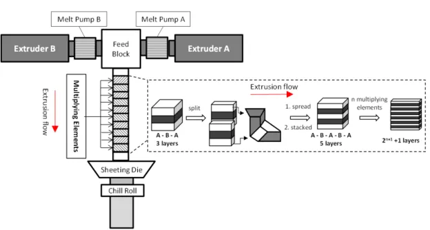
PS–PMMA nanolayered films are manufactured using a multilayer coextrusion process. The processing route consists of two 20-mm single-screw extruders with melt gear pumps, a three-layer coextrusion feed-block (A-B-A), a series of three-layer-multiplying elements, an exit flat die and a thermally regulated chill roll as illustrated in Fig.1.1. PMMA was extruded to form the outer skin layers and PS the core layer. The inclusion of gear pumps into the coextrusion system enables an additional degree of control over the relative thickness ratio of the layered polymers as they enter the A-B-A feed-block. In this study, the mass fraction of polymer B in the film was set and kept constant by adjusting the flow rate through the speed of the melt gear pumps. The initial three-layer polymer flow subsequently enters a mixing section, composed of a sequence of layer-multiplying elements. The melt was initially cut in half vertically, and then each half was compressed and restretched to its original width, hence doubling the number of layers with each layer-multiplying element. A series of n elements combines two polymers producing2n+1+ 1 alternating layers, as shown in Fig.1.1.
Here, 10 multiplying elements were used, giving films containing 2049 layers. Finally, after passing through the last layer-multiplying element, the nanolayered structure was formed into a thin sheet by passing through a flat die, 150 mm wide and 1.5 mm thick. At the die exit, the
Figure 1.1: Principle of the multiplication of layer by the multilayer coextrusion process to fabricate the films
nanolayered samples were stretched and quenched, using a water-cooled chill roll at 95◦C , and collected. The resulting sample is a rectangular film made of alternating layers of PS and PMMA, architectured as a one-dimensional (1D) stacking. The sample has PS/PMMA compositions by weight of 10/90 and a thickness of approximately 250 µm. Based on these parameters, the nominal PS layer thickness is 27 nm (Eq.1.18) and the theoretical volume fraction is 11%.
Nominal thicknessPS=Nominal thicknessFilm VV
PS
Number of layersPS (1.18)
Characterisation techniques
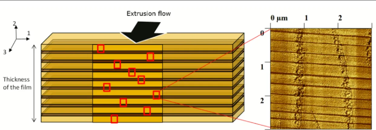
AFM images were obtained in tapping mode using a multimode microscope controlled by a Nanoscope V controller (Veeco), operated under ambient atmosphere. The tips (silicon, spring constant 40 N/m, oscillation frequency ca. 300 kHz) were obtained from BudgetSensors. The radius of curvature of the tips was less than 10 nm. Phase, height and amplitude images were acquired simultaneously. Specimens were cut from the centre of the extruded films and sectioned perpendicular to their surface with an ultramicrotome 2088 Ultrotome V (LKB) at a cutting speed of 1 mm/s. Images were recorded at full resolution (4096 × 4096 pixels), with a scan rate of 0.5 Hz. This resolution yields a pixel size of 7 nm. AFM images were taken from extrusion direction. The phase signal was described as a measure of the energy dissipation involved in the contact between the tip and the sample, which depends on a number of factors, including viscoelasticity, adhesion and topography. As these factors are different between PS and PMMA, the thickness of layers was measured from the AFM phase images (Fig.1.2), which most clearly revealed the layered film structure. On the obtained images, PS and PMMA appear in brown and gold colour,
blends
Figure 1.2: AFM specimen and image analysis principle. The arrow represents the extrusion flow direction (left); AFM image of partial cross section of the sample (vertical lines are compression lines due to sample preparation, right).
3 layers 10 layers 30 layers 100 layers 200 layers 300 layers 500 layers
Number of realisations 275 81 28 10 5 3 2
Average sample size (nm) 738 2441 6949 20143 40287 60076 100717
Total number of PS layers 825 810 840 1000 1000 900 1000
Number of measured PS layers 822 808 800 822 822 742 822
Table 1.2: Characteristics of each volume series
respectively.
Image analysis
Since the film has finite dimensions, 10 images of around 100 layers were taken all along the thickness of the film as represented in Fig.1.2. The sample was composed of 1024 PS layers; a large fraction of PS layers (ca. 80%) was measured indeed. In order to determine the RVE, these 10 images were divided into nonoverlapping, neighbour squares of equal size. Thus, due to the regular nature of the microstructure, it was possible to obtain statistical data for more than 100 layers by compiling them. In the end, seven series of images containing respectively 3, 10, 30, 100, 200, 300 and 500 layers of PS were obtained, as shown in Fig.1.3, for the first four series. The horizontal lines on these AFM images were chatter marks due to sample compression during microtoming. The characteristics for each series are given in Table1.2. The number of realisations corresponds to the number of samples considered within one series.
Thicknesses of PS layers were measured from AFM phase images with the image analysis software Gwyddion. Through the software, a phase profile can be extracted showing the variation of phase degree. It is noteworthy that the profile is averaged over 128 pixels whatever be the image size. This integrated height is larger than the thickness of the cut and compression lines,
Figure 1.3: AFM phase images of PMMA/PS (90/10 wt%) film with (A) 100 layers, (B) 30 layers, (C) 10 layers and (D) 3 layers.
which appear during the sample preparation. Moreover, these lines are perpendicular to the layers. Hence, they are included in the profile noise, and the measurements of layer thickness are not affected. Each layer is represented by one peak on the profile. The thickness of each layer is determined according to an arbitrary procedure which consists of measuring the full width at half-maximum height of the peak. This step is similar to a manual threshold. As the thickness of layers is in the range of tens of nanometres, i.e. a few pixels in terms of AFM imaging, it is critical to analyse all possible sources of error. Various types of error can exist in this case: uncertainties of measurement, systematic error, and sampling error. The size of the AFM tip, AFM controller, image compression and acquisition definition were considered as uncertainties of measurement. The manual threshold and bias due to the operator were considered as systematic error. The sampling, which depends on the size of the considered system, i.e. the total number of layers which will be measured, can be a source of error if the number of analysed layers is too small. This last point is fundamental for our study as the sampling error can be related to the RVE size, given the assumptions of statistical homogeneity and ergodicity for the considered material. Both assumptions will be made from now on in order to provide a consistent ground for applying the approach developed by [Kanit et al., 2003]. Tips used have a curvature radius ofR = 10 nm. The in-plane resolution of AFM is related to the radius of curvature of the tip, as well as the vertical detection limit (∆z = 0.1 nmin our case, given by the manufacturer), and the size of the feature being characterised. The in-plane detection limit is approximated by Eq.1.19.
∆x = 2p2R∆z (1.19)
blends with the theoretical value of PS layers (27nm). Therefore, the uncertainty of measurement due to the AFM tip size was considered negligible. To reinforce this assertion, a comparative study has been done with a thinner tip (R = 2 nm) and results regarding the layer thickness were the same. All images were acquired by the same operator with the same AFM controller at a constant image resolution (4096 × 4096 pixels at a scan rate of 0.5 Hz) in order to avoid image resolution bias. However, it is worth noting that the images were acquired with the highest resolution attainable for this AFM apparatus. The acquisition definition can have a crucial importance on measurements if not chosen cautiously. The minimal acceptable resolution can be defined by a criterion, e.g. that one pixel represents less than 10% of the measured feature. AFM images are recorded as raw data, without algorithmic compression, hence no error due to image file compression was considered. Concerning threshold, with this measurement method, the systematic error on thickness was estimated to one pixel. The size of the pixel depends on the size of the image and the resolution. Here, the systematic error was 27000/4096, being 7 nm. Moreover, this measurement method overestimates the value by including the external pixels in the measure. So, for each value measured on the profile, the value of systematic error was subtracted in order to improve accuracy.
1.2.2 Representativity of AFM samples
There are several morphological criteria (granulometry, anisotropy, etc.) that can be used to characterise random structures. We focus here on the spatial arrangement of a given random structure. It is characterised by, at least, three properties: covariance, distance function and anisotropy. Since this work does not deal with multiscale and/or anisotropic models of random structures, we will only consider the covariance. The covarianceC (x, x + h)of random setA is given by:
C (x, x + h) = P {x ∈ A,x + h ∈ A} (1.20) If Ais a stationary random set,C (x, x + h) = C (h). If Ais ergodic,C (h)can be estimated from the volume fraction ofA ∩ A−h:
C (h) = VV(A ∩ A−h) = VV¡A ª ˇh¢ (1.21) The erosion by{x, x + h}results in variations inC (h)which depend on vectorh(modulus|h|and orientationα). The covarianceQ (h)of the complementary random setAccan also be considered, although it does not give any information compared toC (h):
Q (0) = q = 1 − p (1.22)
Q (h) = P ©x ∈ Ac, x + h ∈ Acª = 1 − 2C (0) +C (h) (1.23)
• C (0) = P {x ∈ A} = p; • 1 π Z 4π 0 − µ∂C (h,α) ∂|h| ¶ h=0
dα = SV(A)when the partial derivative remains finite;
• if C (0) − C (h) ' |h|β for h → 0, with0 < β < 1, the boundary of A has a non integer Haussdorf dimensiond = 3 − β, andAis a fractal set;
• C (∞) = p2, the covariance of a stationary ergodic random set reaches a sill, the events are independent;
• For a given orientation α, C (h) reaches a sill at a certain distance aα, or range, that we consider as the characteristic length scale of the random structure:C (aα) = C (∞) =
VV(A)2= p2;
• The presence of multiple scales in the random structure is characterised inflections of the experimental covariance;
• Periodicity of the structure results in periodicity of the covariance.
Correlation functions are useful for studying physical properties within random structures. The centered second-order correlation function can be deduced from the covariance. For the case of a two-phase medium with propertiesZ = Z1whenx ∈ AandZ = Z2whenx ∈ Ac, it yields:
W2(h) = E {(Z (x + h) − E {Z })(Z (x) − E {Z })} = (Z1− Z2)2¡C (h) − p2¢
= (Z1− Z2)2¡Q (h) − q2¢ (1.24)
The integral range An presented in Section1.1.1is obtained from the centered second-order correlation function in this way:
An= 1
D2
Z Z
RnW2(h)dh (1.25)
In the case of concern for this work, i.e. nanolayered polymer blends ideally structured as a 1D stacking, morphological variability is induced in only one direction, the microstructural morphology being constant in both directions 2 and 3. Eqs.1.4and1.5can thus be reformulated as Eqs.1.26and1.27by considering the sample sizeL, or length of the sample, e.g. in µm:
D2Z(L) = D2Z
A1
L (1.26)
withA1, the integral range inRdefined as :
A1= 1
D2Z
Z
blends By adapting Eq.1.16to the 1D case, it yields:
LRVE= A∗1 γ v u u t 4D2 Z ²2 relZ 2 n (1.28)
This RVE size then depends on the point varianceD2Z, integral range A1and mean value Z . These three parameters are estimated from the image analytically, except when considering the volume fraction which is equal to the length fractionLL, for whichD2Z is known explicitly:
D2LL= LL(1 − LL) (1.29)
For the specific case of PS layer thickness, the theoretical thickness can be obtained from the length fraction as follows:
tth= LLNL (1.30)
withL, size of the sample andN, the number of PS layers within the sample, which is a constant imposed by the number of multiplying elements used during the coextrusion process and the sample sizeL. Hence, Eq.1.31can be adapted in the following way for the point variance of PS layer thickness: D2t = µL N ¶2 LL(1 − LL) (1.31)
The coefficientA∗1 and scaling-law exponentγcan be estimated from image analysis as it was done by [Kanit et al., 2003], [Altendorf et al., 2014] and [Wang et al., 2015], by considering the ensemble varianceD2Z(L)versusLand identifying the ordinate at the origin for the scaling law, hence yieldingD2ZA∗1γfrom which exponentγand point varianceD2Z are known, leaving only
A∗1 to be evaluated. Furthermore, Eq.1.17can be updated for present problem:
D2Z(L) = K L−γ (1.32)
withK = D2ZA∗1γ, leaving only two parameters to be identified from the statistical analysis. Eq.1.28can thus be updated in this way:
LRVE= γ v u u t 4K ²2 relZ 2 n (1.33)
1.2.3 Results and discussion
Morphological measurements have been performed on the six different populations of sample size.
Figure 1.4: Mean values for the PS layer thicknesst (a) and volume fractionLL (b) varying with sample size.
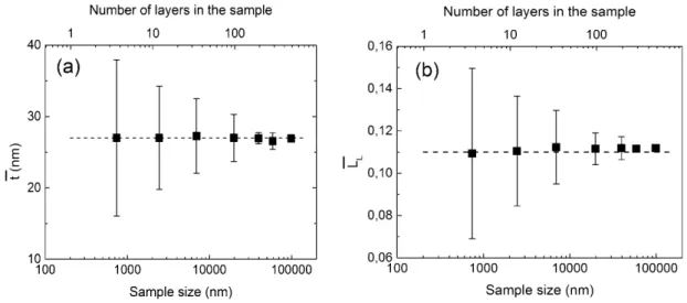
Mean value and distribution
The mean volume fraction of PS layersVV is equal to both the surface fractionSS and length fractionLL of PS, since the microstructural morphology is stationary. LL has been computed over n realisations for a given sample size L in nm. The mean PS layer thickness t was also estimated from image analysis with respect to the size of the sample. BothLL andt are plotted as functions of the sample size in Fig.1.4. The mean values obtained for the largest sample size considered (L = 98862nm) are LL = 11.19 ± 0.03% for the volume fraction and
t = 26.9 ± 0.1nm. Morphological fluctuations are inherent to the stochastic nature of real-life materials. As expected, no bias occurs for both the layer thickness and volume fraction, whatever the size of the realisations.
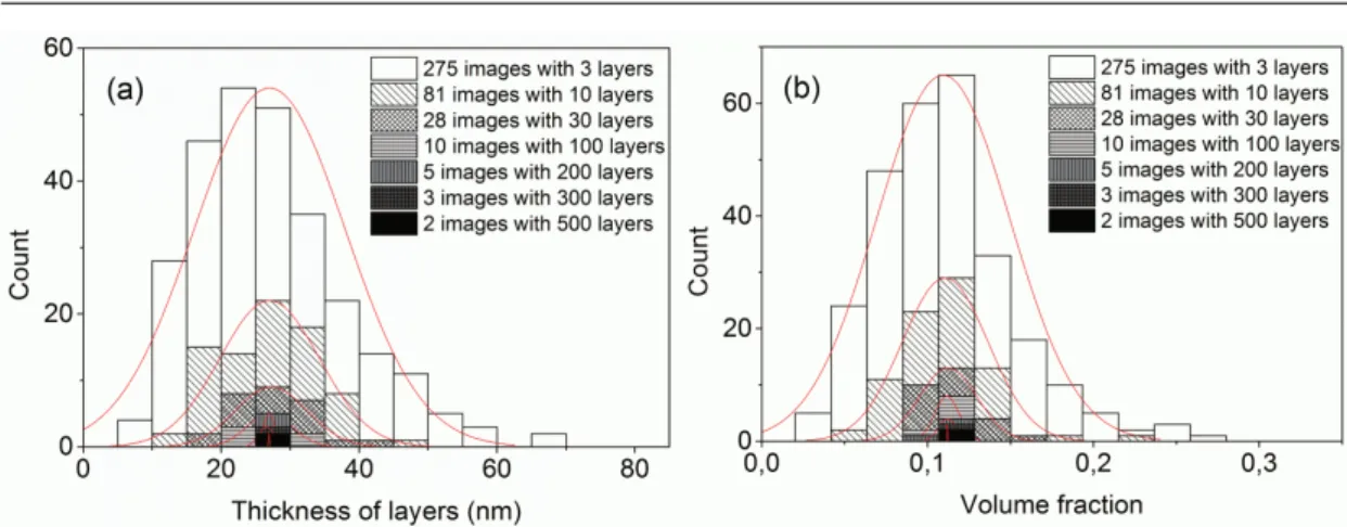
The observed distributions of thickness and volume fraction of PS layers for each sample sizeL
are shown in Fig.1.5(a) and (b), respectively. For each property, the distributions were similar whatever be the considered system. As represented in red lines in Fig.1.5, normal distribution curves have been fitted to the experimental data. Experimental data and fit are in good agreement. For each population, the mean value of the normal distribution curve was equal tot. This result confirms the implicit hypothesis of standard deviation calculation made with Eq.1.12from which the statistical analysis is done.
Covariance
In order to check for morphological regularity of the material considered, the two-point geometri-cal covariance was computed for the sample shown in Fig.1.6(a), which was transformed into the binary image (Fig.1.6(b)) by manual thresholding and morphological opening and closure operations. The considered sample was approximately2 × 2µm, including seven PS layers and a
blends
Figure 1.5: Distribution of statistical population as a function of (a) thickness of layers and (b) volume fraction. The red lines represent the normal distribution curves.
Figure 1.6: (a) AFM micrograph used for the covariance study and (b) binary image for computing the covariance.
volume fraction of PS layers of 11.4%.
Its covariance was estimated along the horizontal direction, the orientation of vectorh, which corresponds to direction 2 in Fig. 1.2. The regular quasi-periodic character of the material is clearly apparent on the covariance plot shown in Fig.1.7, yielding a distance of 280 nm between the centres of two neighbouring PS layers. The first pointC0corresponds to the volume fraction of the sample:VV = 0.114, whereas the sillC∞corresponds toVV2= 0.013.
Morphological representativity
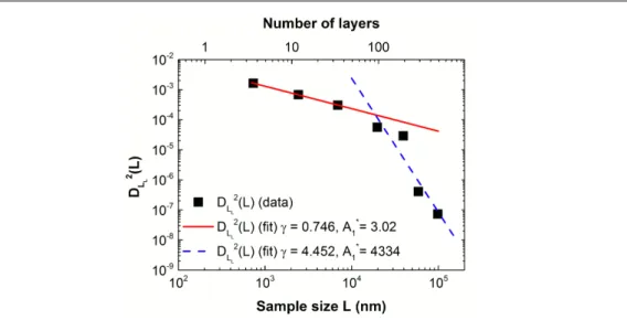
Results regarding the volume fraction are presented in Fig.1.8. Variance for the mean PS layer thickness as a function of the sample size is shown in Fig.1.9. Theγexponents of the scaling law for each morphological property were estimated from the results of image analysis, by fitting the slope of the variance curves. Values of K are estimated from Fig.1.8 and1.9based on Eq.1.32. From Fig.1.8, two slopes are identified for the power law, indicating the existence of
Figure 1.7: Covariance computed horizontally on the image shown in Fig.1.6(b).
two scales of heterogeneities. The first-scale, or local, variability is intrinsic to the microstructure induced by the extrusion process: it encompasses the effects of short-range physical phenomena, such as flow nonlinearities, local thermal inhomogeneity and interfacial interactions. This first scale of variability is always present although its effects become blunter for a larger system; it is characterised by a consistentγexponent of0.66 − −0.75for both properties, which should be compared to the theoretical value of 0.5 obtained for random fibres in 2D [Jeulin, 2016]. The second scale of variability to consider is seen only for sample sizes higher than104nm; its origin could be described as boundary effect patterns during the process. Indeed, due to higher shear rate prescribed to the melt at the wall while passing through multiplying elements, layers in the vicinity of the wall become thinner than others. If this phenomenon occurs at each multiplying step, the final sample is constituted of patterns with long-range varying layer thickness sequences. The tipping point between the slopes could then be interpreted as the characteristic length of such pattern. In our case, the pattern dimension can be estimated to be2.0 × 104nm, corresponding to approximately 100 layers, i.e. about 10% of the film thickness. Rather than considering this a limitation of the statistical approach invoked for the case of films with finite dimensions, we propose to use this method for the characterisation of microstructural variability, in order to study the effect of process parameters on the quality of nanolayered films. As a matter of fact, this statistical approach allows for the discrimination of multiple sources of variability and interpretation of their physical meaning. The second scale of variability appears to accelerate the statistical convergence with respect to the size of the system, for volume fraction (γ = 4.45), as well as for the mean layer thickness (γ = 4.22). Also such exponents are expected for random media with zero integral range, which is the case for the periodic part of the microstructure, as revealed by the quasiperiodic behaviour of the covariance in Fig.1.7. Nevertheless, in this study, sample series containing 100 layers or more have a low number of realisations (≤ 10). More samples would be necessary in order to obtain a better accuracy for these series.
Using Eq. 1.33, it is now possible to determine statistical RVE sizes from image analysis. Estimates for RVE sizes are presented in Table1.3for the different morphological properties (volume fraction and layer thickness of PS), for various relative errors and numbers of realisations (n = {1;10;50}), using the first-scale variability parameters, since only small size samples are
blends
Figure 1.8: VarianceD2LL(L)of the volume fraction of PS depending on sample sizeL, computed from image analysis.
Figure 1.9: VarianceD2t(L)of the thickness of PS depending on sample sizeL, computed from image analysis.
Z γ K n ²rel LRVE(nm) N PS volume fraction 0.746 7.08 × 10⁻² 1 5% 9.92 × 10⁵ 4043 0.746 7.08 × 10⁻² 10 5% 4.53 × 10⁴ 185 0.746 7.08 × 10⁻² 50 5% 5.24 × 10³ 21 0.746 7.08 × 10⁻² 1 10% 1.55 × 10⁵ 630 0.746 7.08 × 10⁻² 10 10% 7.07 × 10³ 29 0.746 7.08 × 10⁻² 50 10% 8.17 × 10² 3 PS layer thickness 0.663 9.43 × 10³ 1 5% 3.23 × 10⁶ 13173 0.663 9.43 × 10³ 10 5% 1.00 × 10⁵ 409 0.663 9.43 × 10³ 50 5% 8.85 × 10³ 36 0.663 9.43 × 10³ 1 10% 4.00 × 10⁵ 1628 0.663 9.43 × 10³ 10 10% 1.24 × 10⁴ 51 0.663 9.43 × 10³ 50 10% 1.09 × 10³ 4
Table 1.3:LRVEsize estimated using Eq.1.33for PS volume fraction and layer thickness.
readily accessible with AFM. RVE sizes presented in this table forn = 1are always larger than the volume element sizes achieved throughout this work: L = 100µmon average for the largest. Nevertheless, the precision for a given sample size can be obtained from multiple realisations of smaller samples. As an example, for tPS, ifL = 12µm, and²rel= 10%, one must analyse
10 realisations in order to obtain the same statistical convergence as for one realisation with
L = 400µm. Precaution should be taken regarding the bias induced by boundary layer effects on mean values by choosing smaller elementary samples when considering physical properties rather than morphological ones.
From both practical and acquisition time viewpoints, for mean value and distribution of layer thickness for a given precision, it is better to analyse images with fewer layers. So, the power-law parameters to be considered for the determination of a representative sample size are those related to the first-scale variability. In order to characterise long-range boundary effects due to the manufacturing process, large samples have to be considered. Such image acquisition might be inaccessible through AFM, and therefore large samples can be reconstructed from smaller contiguous nonoverlapping samples, as it was done in this work.
1.2.4 Conclusions and perspectives
Nanolayered PS–PMMA polymer blend films were manufactured and morphologically charac-terised through AFM and image analysis. Representativity of hundreds of nanoscale heteroge-neous samples was investigated. The statistical approach introduced by [Kanit et al., 2003] was adapted and implemented for the case of 1D nanolayered materials based on image analysis of microstructural samples. RVE sizes were determined for both PS volume fraction and mean
layer thickness. The study of the ensemble variance convergence with respect to the size of the system revealed two regimes for the scaling power law, indicating the presence of two scales of morphological heterogeneities within the material.
In summary, three functions are enabled by the present approach:
• To predict RVE size for a given property and precision;
• To reach the same precision with either one large sample or several smaller samples;
• To discriminate and characterise multiple scales of variability in heterogeneous media.
Further work will include the morphological modelling of such materials in order to generate populations of virtual samples for computation of physical properties, e.g. mechanical, thermal, electrical, etc. As the rate of statistical convergence with respect to the size of the system informs us about variations induced in the microstructure, the current approach will be applied for different factors of influence, i.e. blend compositions, morphologies and process parameters. This work is a useful step further towards understanding the relationship between process parameters, induced microstructures and functional properties.
1.3
RVE size determination for viscoplastic properties in
polycrys-talline materials
Another case of application appeared during the PhD work of Shaobo Yang [Yang, 2018,
Yang et al., 2019] concerned with the study of the dissipative behaviour of polycrystalline copper in very high cycle fatigue regime. In order to compare and interpret experimental results, we resorted to polycrystalline aggregate simulations using finite element analysis. To validate the approach, the representativity of our simulations had to be assessed, which is the aim of the present section.
1.3.1 Introduction
In the past decades, full-field numerical simulation of polycrystalline materials based on fi-nite element analysis has been widely developed to investigate the mechanical behaviour, allowing the analysis of stress and strain fields at a scale that is not easily assessable ex-perimentally [Barbe et al., 2001, Roters et al., 2011]. Most of the authors in the literature dedicated to the simulation of polycrystals usually consider a population of virtual poly-crystalline samples made of several hundred grains, validating this arbitrary choice by analysing the mean value and standard deviation for a given property computed on such population [Shenoy et al., 2007, Shenoy et al., 2008, Robert et al., 2012, Martin et al., 2014,
of full-field simulation of polycrystalline materials results in shedding new light on the rela-tionship between the microstructural description at the dislocation or grain scale and the local mechanical behaviour [Cailletaud et al., 2003]. The homogenised macroscopic response of a polycrystalline material sample will depend on its size, hence yielding the question of representa-tivity for such virtual samples.
Using this approach, [Kanit et al., 2003] studied the RVE sizes of a two-phase 3D Voronoi mosaic for linear elasticity, thermal conductivity and volume fraction, under uniform displacement, traction and periodic boundary conditions (PBC). The results showed that the PBC held an advantage of convergence rate of the mean apparent properties in comparison to other boundary conditions, due to the vanishing of boundary layer effects. A slow rate of convergence for the considered properties would yield a large RVE sizes [Dirrenberger et al., 2014]. Also considering the large calculation cost in the case of crystal plasticity, it is preferable to rely on PBC in order to optimise the computation strategy, as it was done in other investigations [Pelissou et al., 2009,
Jean et al., 2011a].
The statistical method of [Kanit et al., 2003] was implemented for the estimation of RVE size, not only for linear mechanical properties and morphological property, but also for plastic properties: [Madi et al., 2006] evaluated the RVE size for 2D/3D viscoplastic composite materials. In their study, the macroscopic strain rate of the 2D/3D material was modeled using a Norton flow rule. Based on the von Mises criterion, an apparent viscoplastic parameterPvappwas firstly defined as the coupling of two parameters of the Norton flow ruleK andn, i.e.Pvapp=K1n. The authors showed that the value of Pappv converged towards a constant value with an increasing volume of simulation and that the RVE size forPvappwas found to be smaller than the ones for elastic moduli. In the present study, we relied on this definition of the apparent viscoplastic parameter, as it is adapted for describing the nonlinear behaviour of a macroscopically isotropic polycrystalline viscoplastic material.
As a matter of fact, the concept of RVE has often been used in investigations associated with the average mechanical response of 2D and 3D polycrystalline material. The definition of RVE size can stem from finite element meshing considerations or convergence of mean values for a considered property. For instance, [Barbe et al., 2001] described the RVE for a cubic polycrys-talline mesh as an equilibrium between the number of grains (238) and the average number of integration points per grain (660) attainable within typical computational means. More recently, [Sweeney et al., 2015] estimated the energetic parameter of CoCr stent material in high cycle fatigue by averaging in 5 RVEs with 138-140 grains. [Cruzado et al., 2017,Cruzado et al., 2018] simulated the cyclic deformation of metallic alloys with 20 RVEs and a size of 300 grains, which showed an error less than 10% for elastoviscoplastic properties. Similar determination of mate-rial RVE size can also be found in [Shenoy et al., 2007,Shenoy et al., 2008,Martin et al., 2014,
Gillner and Münstermann, 2017, Teferra and Graham-Brady, 2018]. In these references, RVE size is defined as a few realisations with a few hundred grains which can realise a convergence of mean properties. However, these analyses do not allow for a rigorous statistical definition of the
RVE size.
Rather than relying solely on the convergence of mean properties, the method proposed in [Kanit et al., 2003] makes use of the rate of convergence of the ensemble variance of the mean properties with respect to the volume size, thus enabling the definition and estimation of a statistical RVE size for each considered property. However, no one ever assessed the RVE size for polycrystalline material in the framework of CPFEM with the statistical RVE method. Additional consideration has to be made regarding the apparent properties to be considered as criteria for RVE size determination in viscoplasticity. The first one should be the definition of intrinsic dissipation within the context of crystal plasticity. Secondly, the definition of the apparent viscoplastic parameter will be considered in the crystal plasticity framework. Meanwhile, for the crystal plasticity behaviour, material heterogeneity is mainly due to the local grain orientation, which can introduce strong stress concentrations, leading to early onset of plasticity. Both grain orientation and the choice of crystal plastic behaviour are likely to influence directly the value of RVE size for mechanical properties, as it will be discussed in the paper.
1.3.2 Crystal plasticity constitutive model
The material involved in this paper was pure polycrystalline copper. Both anisotropic crystal elasticity and plasticity were considered for its behaviour. The cubic elasticity is characterised by 3 independent elastic constants, taken from [Musienko et al., 2007]. The crystal plasticity model considered in the present work was introduced and implemented by [Méric et al., 1991,
Cailletaud, 1992] in the finite element code ZeBuLoN/ZSet1. The Meric-Cailletaud model was chosen for its ability to account for kinematic hardening. This model is popular within the crystal plasticity community and has been used in many previous works on computational mechanics for polycrystalline material [Barbe et al., 2001,Diard et al., 2005,Gérard et al., 2009]. For the sake of conciseness, the crystal plasticity model and its parameters will not be presented here, for more details the enquiring reader can refer to [Yang et al., 2019].
1.3.3 Computational approach
Periodic three-dimensional mesh generation
In this paper, a methodology is employed for generating and meshing 3D random polycrystals. The associated mesh optimisation approach and statistical work of mesh quality are fully presented in the reference paper [Quey et al., 2011]. The corresponding algorithms are implemented and distributed in an open-source software package: Neper2. Using Neper, the Voronoi tesselation can be constructed with a periodicity constraint, needed for PBC. For the sake of simplicity and comparison with results from the literature, an isotropic morphological and crystallographic texture is considered. To do so, the three Euler-Bunge angles (α,β,γ) in the Z-X-Z type are
1http://www.zset-software.com 2http://neper.sourceforge.net/
![Figure 2.2: Characteristic lengths associated with architectured materials and different fields of interest for materials, adapted from [Bouaziz et al., 2008]](https://thumb-eu.123doks.com/thumbv2/123doknet/14463922.713163/57.892.121.712.150.544/figure-characteristic-associated-architectured-materials-different-materials-bouaziz.webp)
