HAL Id: hal-01465110
https://hal.archives-ouvertes.fr/hal-01465110
Submitted on 12 Dec 2018
HAL is a multi-disciplinary open access
archive for the deposit and dissemination of
sci-entific research documents, whether they are
pub-lished or not. The documents may come from
teaching and research institutions in France or
abroad, or from public or private research centers.
L’archive ouverte pluridisciplinaire HAL, est
destinée au dépôt et à la diffusion de documents
scientifiques de niveau recherche, publiés ou non,
émanant des établissements d’enseignement et de
recherche français ou étrangers, des laboratoires
publics ou privés.
Frequent Itemset Border Approximation by Dualization
Nicolas Durand, Mohamed Quafafou
To cite this version:
Nicolas Durand, Mohamed Quafafou. Frequent Itemset Border Approximation by Dualization.
Trans-actions on Large-Scale Data- and Knowledge-Centered Systems, Springer Berlin / Heidelberg, 2016,
26, pp.32-60. �hal-01465110�
Dualization
Nicolas Durand and Mohamed Quafafou
Aix Marseille Universit´e, CNRS, ENSAM, Universit´e de Toulon, LSIS UMR 7296, 13397, Marseille, France
{nicolas.durand,mohamed.quafafou}@univ-amu.fr http://www.lsis.org
Abstract. The approach F IBAD is introduced with the purpose of computing approximate borders of frequent itemsets by leveraging du-alization and computation of approximate minimal transversals of hy-pergraphs. The distinctiveness of the F IBAD’s theoretical foundations is the approximate dualization where a new function ef is defined to compute the approximate negative border. From a methodological point of view, the function ef is implemented by the method AM T HR that consists of a reduction of the hypergraph and a computation of its min-imal transversals. For evaluation purposes, we study the sensibility of F IBAD to AM T HR by replacing this latter by two other algorithms that compute approximate minimal transversals. We also compare our approximate dualization-based method with an existing approach that computes directly, without dualization, the approximate borders. The experimental results show that our method outperforms the other meth-ods as it produces borders that have the highest quality.
Keywords: frequent itemsets, borders, hypergraph transversals, dual-ization, approximation.
1
Introduction
The discovery of frequent itemsets was initiated by Agrawal et al. [3]. This research field has quickly become an important task of data mining. The problem is to find the sets of items (i.e. attribute values) that appear together in at least a certain number of transactions (i.e. objects) recorded in a database. These sets of items are called frequent itemsets. In that regard, other types of itemsets have been proposed, for instance, closed itemsets [33], free itemsets [8] and emerging itemsets [11]. Even more important, such itemsets play a key role in the generation of association rules [3], supervised classification [34], clustering [14] and are useful in a broad of range of application fields [22].
Two issues are important in the discovery of frequent itemsets: (1) the re-duction of the search space due to combinatorial explosion and (2) the rere-duction of the number of generated itemsets to improve efficiency. In this paper, we consider only the second point, with a focus on the set of maximal frequent
itemsets corresponding to a subset of frequent closed itemsets [33]. The max-imal frequent itemsets represent a reduced collection of frequent itemsets, but they are not considered as a condensed representation contrary to the frequent closed itemsets. Indeed, the regeneration of all the frequent itemsets is possible from the maximal frequent itemsets but the database must be read to compute the frequencies. The problem of mining maximal frequent itemsets is NP-hard [40]. The algorithms discovering these itemsets are, for instance, M axM iner [5], P incer-Search [29], M AF IA [9], GenM ax [20], Dualize&Advance [21], IBE [37] and ABS [18]. Maximal frequent itemsets are used a lot in recommendation systems where long itemsets describe trends. For example, a list of movies (i.e., a maximal itemset) that many people like can be used as recommendations for other users that share a large overlap of movies with this list.
The maximal frequent itemsets and the minimal infrequent itemsets corre-spond respectively to the positive border and the negative border of the set of frequent itemsets [30]. These two borders are linked together by the computa-tion of minimal hypergraph transversals (also called ”minimal hitting sets”) [30, 10]. Thus, it is possible to switch to a border from the other one. This is called dualization. Algorithms like Dualize&Advance [21], IBE [37] and ABS [18] use dualization to discover maximal frequent itemsets. Indeed, Dualize&Advance computes the maximal frequent itemsets one by one, IBE is an improvement of the previous algorithm as it avoids the redundant frequency checks, and ABS starts computing the positive border and uses an adaptative strategy to decide when it is interesting to switch to the other border. Let us remark that the number of itemsets of the borders can be huge.
This paper extends our previous work in [15]. We propose the approach F IBAD1with the purpose of computing approximate borders of frequent item-sets by leveraging dualization and computation of approximate minimal transver-sals of hypergraphs. The aim is to reduce the size of borders. The originality of the proposed approach comes from a new fonction we have defined to com-pute approximate negative borders. From a methodological point of view, the function is implemented by the method AM T HR2 that consists of a reduction of the hypergraph and a computation of its minimal transversals. Next, the ap-proximate positive borders are computed from the apap-proximate negative borders by an exact function. To the best of our knowledge, this is the first time that such approach is proposed leveraging dualization and border approximation. For evaluation purposes, we conduce experiments realized on different data sets, and evaluated the quality of the computed approximate borders by using the distance between the computed approximate borders and the exact ones. Morevover, we study the sensibility of F IBAD to AM T HR. For this, we replace AM T HR with two other methods that compute approximate minimal transversals. We also compare our dualization-based method with an existing approach which computes directly, without dualization, the approximate positive borders.
1 Frequent Itemset Border Approximation by Dualization 2
The rest of the paper is organized as follows. Section 2 defines notations and basic notions necessary for understanding the paper. Related works are discussed in Sect. 3. The proposed approach is detailed in Sect. 4. Section 5 presents our method that computes approximate minimal transversals. The experiments and the results are presented in Sect. 6. We conclude and present some future work in Sect. 7.
2
Preliminaries
Let D = (T , I, R) be a data mining context, T a set of transactions, I a set of items (denoted by capital letters), and R ⊆ T × I is a binary relation be-tween transactions and items. Each couple (t, i) ∈ R denotes the fact that the transaction t is related to the item i. A transactional database is a finite and nonempty multi-set of transactions. Table 1 provides an example of a transac-tional database consisting of 6 transactions (each one identified by its ”Id”) and 8 items (denoted A . . . H).
Table 1. Example of transactional database. Id Items t1 A C E G t2 B C E G t3 A C E H t4 A D F H t5 B C F H t6 B C E F H
An itemset is a subset of I (note that we use a string notation for sets, e.g., AB for {A, B}). The complement of an itemset X (according to I) is noted X. A transaction t supports an itemset X iff ∀i ∈ X, (t, i) ∈ R. An itemset X is frequent if the number of transactions which support it, is greater than (or is equal to) a minimum threshold value, noted minsup. The set of all-frequent itemsets, noted S, is presented in Definition 1.
Definition 1 (Set of all-frequent itemsets).
Let D = (T , I, R) be a data mining context and minsup be the minimum thresh-old value. The set of all-frequent itemsets, noted S, is:
S = {X ⊆ I, |{t ∈ T , ∀i ∈ X (t, i) ∈ R}| ≥ minsup}.
The notion of frequent itemset border was introduced by Mannila & Toivonen in [30] (see Definition 2). The borders can be visualized by using the itemset lattice, i.e., the partial order naturally defined on the powerset of I (see Fig. 1). The itemset lattice represents the complete search space.
Fig. 1. Lattice of all subsets of items of I
Definition 2 (Positive border and negative border). The set of all maxi-mal frequent itemsets (resp. minimaxi-mal infrequent itemsets), w.r.t. set inclusion, in D is the positive border (resp. negative border) of S and is noted Bd+(S) (resp. Bd−(S)).
Bd+(S) = {X ∈ S | ∀Y ⊃ X, Y /∈ S}. Bd−(S) = {X ∈ 2I\ S | ∀Y ⊂ X, Y ∈ S}.
Example 1. Let us take the example of Table 1, if minsup=3 then the itemset H is frequent because 4 transactions support it (t3, t4, t5 and t6). AE is not frequent because only t1 and t3 support it. The set of all-frequent itemsets is S = {A, B, C, E, F, H, BC, CE, CH, F H}. The positive border and the negative border are: Bd+(S) = {A, BC, CE, CH, F H} and Bd−(S) = {D, G, AB, AC, AE, AF, AH, BE, BF, BH, CF, EF, EH}.
Before the presentation of the relationship between the positive border and the negative border of frequent itemsets, we need to introduce the notion of hypergraph (see Definition 3), the notion of simple hypergraph (see Definition 4) and the notion of minimal transversals of a hypergraph (see Definition 5) [6]. Definition 3 (Hypergraph and degree of a vertex). A hypergraph H = (V , E) is composed of a set V of vertices and a set E of hyperedges [6]. Each hyperedge e ∈ E is a set of vertices included or equal to V . The degree of a vertex v in H, denoted degH(v), is the number of hyperedges of H containing v. Definition 4 (Simple hypergraph and minimal hyperedges). Let H=(V , E) be a hypergraph. H is simple if for every pair ei, ej ∈ E, ej ⊆ ei ⇒ j = i. min(H) is the set of minimal hyperedges of H w.r.t. set inclusion, i.e., min(H) = {ei∈ E|(∀ej∈ E, i 6= j, ej⊆ ei) : ej = ei)}. The hypergraph min(H) is simple. Definition 5 (Transversal and minimal transversal). Let H be a hyper-graph and τ be a set of vertices (τ ⊆ V ). τ is a transversal of H if it intersects all the hyperedges of H. A transversal is also called a ”hitting set”. The set of all the transversals of H is T r(H) = {τ ⊆ V | ∀ei∈ E, τ ∩ ei6= ∅}. A transversal τ of H is minimal if no proper subset is a transversal of H. The set of all minimal transversals of H is noted M inT r(H).
The following Proposition 1 results from the definition of the minimal transver-sals of a hypergraph. Considering a hypergraph H, the minimal transvertransver-sals of H are the same as the minimal transversals of the set of minimal hyperedges of H [28].
Proposition 1. Let H=(V , E) be a hypergraph. Then, M inT r(H) is a simple hypergraph and M inT r(H) = M inT r(min(H)).
Fig. 2. The hypergraph from the example of Table 1
Example 2. Let us consider the example of Table 1 as a hypergraph H. The transactions are the hyperedges and the items are the vertices (see Fig. 2). Here, min(H) = {t1, t2, t3, t4, t5}. The set of vertices BC is not a transversal. ABC is a transversal but is not minimal (by removing B, it remains a transversal). AC and EF are minimal transversals. The set of all minimal transversals of H is {AB, AC, CD, CF, CH, EF, EH, GH, AF G, BDE}.
The computation of the negative border from the positive border and vice versa are presented in Property 1 [30] and Property 2 [10].
Property 1 (Negative border and minimal transversals)
Bd−(S) = M inT r(Bd+(S)) where Bd+(S) is the hypergraph formed by the items of I (i.e. the vertices) and the complements of the itemsets of the positive border of S (i.e. the hyperedges).
Property 2 (Positive border and minimal transversals)
Bd+(S) = M inT r(Bd−(S)) where Bd−(S) is the hypergraph formed by the items of I (i.e. the vertices) and the itemsets of the negative border of S (i.e. the hyperedges).
Example 3. Let us compute Bd−(S) from Bd+(S) with our running example. Bd−(S) = M inT r(Bd+(S)) = M inT r({A, BC, CE, CH, F H})
= M inT r({BCDEF GH, ADEF GH, ABDF GH, ABDEF G, ABCDEG}) = {D, G, AB, AC, AE, AF, AH, BE, BF, BH, CF, EF, EH}.
Let us compute Bd+(S) from Bd−(S). Bd+(S) = M inT r(Bd−(S)) = M inT r({D, G, AB, AC, AE, AF, AH, BE, BF, BH, CF, EF, EH}) = {BCDEF GH, ADEF GH, ABDF GH, ABDEF G, ABCDEG} = {A, BC, CE, CH, F H}.
The term dualization refers to the use of the two previous properties to com-pute the negative border from the positive border, and vice versa.
Due to the exponential size of the search space, the size of the borders can be huge according to minsup. In this paper, we propose an approach to approximate the borders and to reduce their size. In this way, the exploitation of the itemsets of the borders will be easier. The next section presents the related works and positions our propositions.
3
Related Works
3.1 Approximation of the Frequent Itemset Border
The approximation of both positive and negative borders of frequent itemsets has been examined on the basis algorithmic dimension [7]. At first, the computation of the approximate borders is performed directly from the data. In fact, it was shown that there is no algorithm of approximation to compute the positive border with a reasonable approximation factor. Furthermore, the computation of the negative border can be approximated by a greedy algorithm in polynomial time.
Numerous methods have been proposed to reduce the number of itemsets of the positive border. In [23], the authors have proposed an algorithm to obtain k representative itemsets by uniformly sampling from the pool of all maximal frequent itemsets (i.e., the positive border). They have used a variant of Markov Chain Monte Carlo algorithm. The algorithm simulates a random walk over the frequent itemset partial order graph with a prescribed transition probability matrix, whose values are computed locally during the simulation. In [31], the au-thors have studied the problem of randomly sampling maximal itemsets without explicit enumeration of the complete itemset search space. They have employed a simple random walk that only allows additions of singletons to the current set untill a maximal itemset is found. An approximation measure, given as input of the algorithm, is used to guide the search for maximal frequent itemsets to different parts of the output space.
In [2], the approximation of a collection of frequent itemsets by the k best covering sets has been studied. The proposed algorithm input is the whole collec-tion of the frequent itemsets or the positive border. The authors have explained the difficulties to use a greedy algorithm to obtain k covering sets belonging to
the initial collection. In [41], the authors have proposed the notion of colossal fre-quent itemsets. Some small frefre-quent itemsets (defined as core itemsets) are fused into colossal itemsets by taking leaps in the itemset search space. The fusion pro-cess is designed to give an approximation to the colossal frequent itemsets. The maximal number of colossal itemsets to discover is given as input. In [25], the authors have proposed a concise representation for a collection of frequent item-sets, called cartesian contour, based on the cartesian product. They have linked the computation of the cartesian contour into a generalized minimum biclique cover problem and they have designed an approximate algorithm with bound. This algorithm takes in input the set of all maximal frequent itemsets and pro-duces a cover. Let us remark that, with this approach, there is no need to set the number of itemsets, contrary to the previous presented works.
Other approaches exist to reduce the number of itemsets but the link with maximal frequent itemsets is not direct. In [39], the authors have used the Min-imum Description Length (MDL) principle: the best set of itemsets is that set that compresses the database best. A post-treatment step would be needed to obtain maximal itemsets.
Our approach computes an approximate border from a border given as input. In that respect, other algorithms presented in [2] and [25] have borders as input. Nevertheless, we do not try to find some covering sets, but our primary goal is to approximate the border that may contains itemsets, which are not necessarily belong to the initial collection. Our approach has the advantage to generate both the approximate positive border and the corresponding approximate negative border. We have an understanding mapping between the exact border and the approximate border. Consequently, we have the possibility to use several other strategies to approximate borders (see Sect. 4). Moreover, contrary to the most of the previous presented works, we do not need to fix the size of the searched borders.
3.2 Approximate Minimal Transversals
The computation of minimal transversals is a central point in hypergraph theory [6] and represents a NP-hard problem. The algorithms that address this need have been developed by different communities like graph theory [6, 28], logic [19, 16] and data mining [12, 4, 24]. Some works approximate the minimal transversals in order to obtain several ones or only one [36]. Some works are based on an evolutionary computation [38] where the transversality and the minimality are transcribed both in a fitness function.
In [1], the Staccato algorithm computes low-cost approximate minimal trans-versals with a depth-first search strategy. It has been designed for model-based diagnosis. We have adapted Staccato in order to compute approximated mini-mal transversals in general and to use it in the experiments (see Sect. 6). The adaptation consists of defining the Staccato’s cost function using properties of vertices belonging to the hypergraph (i.e., their degrees). This adaptation al-lows the definition of vertex’s cost. The algorithm sorts the vertices according to their cost value in decreasing order. This vertex ranking is exploited to guide
the search. At each selection step, only the first λ (%) vertices of the remaining hypergraph are used. For instance, the algorithm starts by selecting the vertex having the highest cost value. Then, it selects the vertex having the highest cost value in the hypergraph formed by the hyperedges not intersected yet. Etc. The more the λ value is high, the more the result is close to the set of all minimal transversals.
The algorithm presented in [35], that we call δ-M T miner in reference to M T miner [24], produces minimal transversals which can miss at most δ hy-peredges. It uses a breadth-first search strategy and several itemset discovery techniques (candidate generation, anti-monotone constraint, . . . ). The search space corresponds to the lattice of all subsets of items (i.e., the vertices). The transactions correspond to the hyperedges. The algorithm uses the notion of ”anti-support”, where the anti-support of an itemset is the number of transac-tions having no item in common with this itemset. If the anti-support of an item-set is equals to 0 then this itemitem-set is a transversal. The minimality is achieved by using free itemsets [8]. A δ-minimal transversal is a free itemset having an anti-support lower than or equals to δ. Let us note that δ-M T miner is especially efficient on dense hypergraphs (i.e., hypergraphs which strongly intersect).
Staccato and δ-M T miner present two approaches to compute approximate minimal transversals. Alternatively, we propose a method that performs a hyper-graph reduction and then computes the minimal transversals of the reduced hy-pergraph. These transversals are considered as the approximate minimal transver-sals of the initial hypergraph. The number of missed hyperedges is free, contrary to δ-M T miner. Moreover, using our method, there are no parameters to set in advance.
3.3 Hypergraph Reduction
The classical approaches to reduce a hypergraph are edge and hyperedge coars-ening [27]. In the edge coarscoars-ening approach, pairs of vertices that are present in the same hyperedges are selected to group the vertices. On the contrary, in the hyperedge coarsening approach, a set of independent hyperedges is selected and the vertices that belong to individual hyperedges are contracted together. The hyperedges are initially sorted, and they are visited according to the re-sulted order. Variants of these two approaches exist. For more information, we refer the reader to [27]. Recently, in [13], two algorithms of hypergraph reduc-tion have been proposed. The first algorithm, called HR-IH, uses hyperedge intersections. Whereas, the second algorithm, called HR-M ST , uses minimum spanning tree. The hypergraph reduction is a step of the proposed hypergraph clustering method which is applied to image segmentation.
Our hypergraph reduction algorithm uses, as HR-IH, the hyperedge inter-sections. Nevertheless, only the step of computation of hyperedge intersections is in common. In fact, HR-IH computes a cover of the set of hyperedge inter-sections and our algorithm selects the most interesting interinter-sections according to a heuristic for finding minimal transversals.
4
Proposed Approach of Border Approximation
The F IBAD approach is introduced with the purpose of computing approximate borders by dualization. Let f and g be the functions that allow to compute re-spectively the negative border from the positive border and vice versa:
f : 2I → 2I
x 7→ M inT r(x)
g : 2I → 2I
x 7→ M inT r(x)
The following diagram allow us to visualize the dualizations between the positive and negative borders:
Bd+(S) f ** Bd−(S) g jj
The principle of F IBAD is to replace the function f by a function ef which performs an approximate computation of the negative border. We define the following new function ef that uses an approximate minimal transversals compu-tation, notedM inT r:g
e
f : 2I→ 2I
x 7→M inT r(x)g
From the positive border, the function ef computes an approximate negative border, notedBdg−(S) (see Definition 6).
Definition 6 (Approximate negative border). Let Bd+(S) be a positive border of frequent itemsets. The approximate negative border, noted Bdg−(S), is defined as follows:
g
Bd−(S) = ef (Bd+(S)) = g
M inT r(Bd+(S)).
The return to a positive border (via the function g) allows to obtain an approximate positive border, notedBdg+(S) (see Definition 7).
Definition 7 (Approximate positive border). Let Bdg−(S) be an approxi-mate negative border of frequent itemsets. The approxiapproxi-mate positive border, noted
g
Bd+(S), is defined as follows:
g
From the positive border, the proposed approach produces the approximate negative border gBd−(S) and the corresponding approximate positive border
g
Bd+(S). The following diagram presents all the dualization process:
Bd+(S) g Bd+(S) e f ** g Bd−(S) g jj
Let us remark that we still have an exact dualization between the two ap-proximated borders: g Bd+(S) f ** g Bd−(S) g jj
In order to give a general overview of F IBAD, we introduce Algorithm 1 by noting that its main Steps 2 and 3 are treatments considered in the next section. Next, we illustrate F IBAD with Example 4.
Algorithm 1 General overview of FIBAD
Require: a positive border of frequent itemsets, Bd+(S)
Ensure: the approximate negative and positive borders,Bdg−(S) andBdg+(S) {Steps 1, 2 and 3: Dualization using function ef }
1: H=Bd+(S); {Computation of the hypergraph from Bd+(S)}
2: HR=HR(H); {Reduction of the hypergraph H}
3: Bdg−(S)=M inT r(H)=M inT r(Hg R) {Computation of the approximate negative
border ; The approximate minimal transversals of H are the exact minimal transver-sals of HR}
{Step 4 and 5: Dualization using function g}
4: P =M inT r(Bdg−(S)); {Computation of the exact minimal transversals ofBdg−(S)} 5: Bdg+(S)=P ; {Computation of the approximate positive border}
6: return Bdg−(S) andBdg+(S);
Example 4. Let us take the example of Table 1 with minsup=3, Bd+(S) = {A, BC, CE, CH, F H}, and let us compute the approximate borders with F IBAD. Step 1: H = Bd+(S) = {A, BC, CE, CH, F H} = {BCDEF GH, ADEF GH, ABDF GH, ABDEF G, ABCDEG}
Steps 2 and 3:Bdg−(S) =M inT r(H) = M inT r(Hg R). Let us assume that this computation provides the following result:Bdg−(S) = {D, E, G, AF, AH, BF, BH}.
Step 4: P = M inT r(Bdg−(S)) = M inT r({D, E, G, AF, AH, BF, BH}) = {ABDEG, DEF GH}
Step 5:Bdg+(S) = P = {ABDEG, DEF GH} = {CF H, ABC}.
We can remark that A, B, C and BC are frequent itemsets and here ABC is considered as a frequent itemset. CF H is not frequent (its support is equal to 2) but it is almost frequent. These two itemsets can be interesting for applica-tions like document recommendation. For instance, without our approach, F H is frequent and CF H is not frequent. The item C is potentially interesting. If the items are documents, with our approach, the item C can be recommended to a user.
In short, the distinctiveness of the F IBAD’s theoretical foundations is the approximate dualization where the new approximate function ef is defined to compute the approximate negative border from the exact positive one. From a methodological point of view, the approximate function is defined as a sequence of two subfunctions: (1) reduction of the hypergraph formed by the comple-ments of the itemsets of the exact positive border (Step 2 of Algorithm 1) and (2) computation of the exact minimal transversals of the reduced hypergraph (Step 3 of Algorithm 1). Thus, the resulted transversals are the approximate minimal transversals of the initial hypergraph. They correspond to the approxi-mate negative border as the input hypergraph is formed by the complements of the itemsets of the exact positive border. Afterwards, the approximate positive border is computed from the approximate negative border by an exact function g. In the remainder of this paper, the sequence of the two subfunctions is called AM T HR and is detailed in the next section.
It should be noted that the function ef can be supported by any other func-tions that compute approximate minimal transversals. The use of each alterna-tive functions, instead of AM T HR, leads to a new strategy for computing ap-proximate borders using dualization. In this paper, the function g is unchanged and its experimental section is dedicated to the comparaison of our proposal with other alternative strategies.
5
Computation of Approximate Minimal Transversals
We propose the method AM T HR to compute the approximate minimal hyper-graph transversals (Steps 2 and 3 of Algorithm 1). This method is based on a new algorithm that reduces the initial hypergraph. Our goal is to compute the minimal transversals on the reduced hypergraph which is smaller than the ini-tial one. The proposed algorithm of reduction is specially designed to compute minimal transversals. It exploits the fact that the hyperedges formed by the complements of the itemsets of the positive border, strongly intersect (i.e. the average degree of a vertex is high). For instance, in Example 4, this hypergraph is: {BCDEF GH, ADEF GH, ABDF GH, ABDEF G, ABCDEG}. The pro-posed method is compro-posed of two steps: (1) Reduction of the hypergraph and (2) Computation of the (exact) minimal transversals of the reduced hypergraph. At the end, the minimal transversals obtained from the reduced hypergraph are declared as the approximate minimal transversals of the initial hypergraph.
5.1 Reduction of the Hypergraph
The reduction method is based on both the intersections of the hyperedges and the degree of each vertex. The representative graph [6] (also called ”line-graph”) of the hypergraph is thus generated. Let us recall that the representative graph of the hypergraph H is a graph whose vertices represent the hyperedges of H and two vertices are adjacent if and only if the corresponding hyperedges in H intersect. In our algorithm, we add values to the edges of the representative graph.
Algorithm 2 presents the reduction of a hypergraph H. This algorithm is composed of three steps: (1) Computation of the degree of each vertex in H (lines 1-3), (2) Generation of the valued representative graph of H (lines 4-9), and (3) Generation of the reduced hypergraph from the valued representative graph (lines 10-17).
Algorithm 2 HR (Hypergraph Reduction)
Require: a hypergraph H=(V , E) where |V |=n and |E|=m Ensure: the reduced hypergraph HR
1: for all v ∈ V do 2: Compute degH(v) 3: end for 4: V0← {v0i} i = 1, . . . , m; {each v 0 i∈ V 0 represents ei∈ E} 5: E0← {}; 6: for all vi0∩ v 0 j6= ∅ do 7: E0← E0∪ {(v0 i, v0j)}; 8: w(vi0,v0j)← P v∈{ψ−1(v0 i)∩ψ−1(v0j)} degH(v); 9: end for 10: VR← {}; 11: ER← {}; 12: while E06= ∅ do
13: Select e0max = (v0maxi, v0maxj) having the maximal weight value
14: VR← VR∪ {ψ−1(v0maxi) ∩ ψ−1(v0maxj)};
15: ER← ER∪ {{ψ−1(v0maxi) ∩ ψ−1(v0maxj)}};
16: Delete the edges e0∈ E0
where v0maxior v0maxjis present
17: end while 18: return HR;
Valued Representative Graph Generation (lines 1-9). Let be H = (V, E) a hypergraph (|V | = n and |E| = m). The algorithm constructs a valued graph G=(V0, E0) where V0 = {vi0} (i = 1, . . . , m) and E0 = {e0
k} (k = 1, . . . , l). A vertex v0i represents a hyperedge ei from H. Let be ψ : E → V0 the bijective function that associates a hyperedge ei to a vertex vi0. A hyperedge between v0i and v0j shows that the intersection between the hyperedges ψ−1(v0i) and ψ−1(v0j)
(ei and ej from H) is not empty. The weight of an edge is based on the degree of each vertex in the corresponding intersection.
To evaluate the weight of a generated edge, we use the degree of each vertex from the initial hypergraph. The idea is that a vertex very present has a good chance to be in a minimal transversal. This expresses a ”degree” of transversality. If the degree of a vertex is equal to the number of hyperedges then this vertex is a minimal tranversal. Let us note that this heuristic is used by several algorithms that compute transversals [1, 36].
The weight of an edge e0k = (v0i, v0j), noted we0
k, is the sum of the degree
of the vertices present in the intersection which has led to create this edge (see (1)). we0 k= X v∈{ψ−1(v0 i)∩ψ−1(v0j)} degH(v). (1)
Generation of the Reduced Hypergraph (lines 10-17). After the creation of the valued representative graph, the algorithm performs a selection of edges with a greedy approach. It selects the edge having the higher weight value while there are edges left in the valued representative graph G. Each selected edge is transformed to a hyperedge of the reduced hypergraph. This hyperedge contains the vertices from H corresponding to the intersection of the two vertices of the edge.
We obtain, at the end, a set of hyperedges corresponding to the reduced hypergraph HR=(VR,ER). Let us remark that if several edges have the same weight, the first edge found is selected.
Example 5. Let us consider the example of Table 1 as a hypergraph H (6 hyper-edges, 8 vertices). The transactions are the hyperedges ek and the items are the vertices vi. First, the degree of each vertex is evaluated: occur[A] = 3, occur[B] = 3, occur[C] = 5, occur[D] = 1, occur[E] = 4, occur[F ] = 3, occur[G] = 2 and occur[H] = 4. Then, the intersections between the hyper-edges are computed. For instance, ψ−1(v10) ∩ ψ−1(v30) = e1∩ e3 = {A, C, E}. The sum of the numbers of occurrences of A, C and E is equals to 12. This is the weight of the edge (v0
1, v30) generated in G. The adjacency matrix of the generated valued graph is:
v01 v02 v30 v04v50 v60 v01 0 11 12 3 5 9 v02 11 0 9 0 8 12 v03 12 9 0 7 9 13 v04 3 0 7 0 7 7 v05 5 8 9 7 0 15 v06 9 12 13 7 15 0
The edge (v50, v06) is selected because its weight is maximal (i.e., 15). The edges where v05 or v06 are present, are deleted. Thus, we have VR = {B, C, F,
H} and ER = {{B, C, F, H}}). The adjacency matrix of the remaining valued graph is: v01 v02 v30 v04v05v06 v01 0 11 12 3 0 0 v02 11 0 9 0 0 0 v03 12 9 0 7 0 0 v0 4 3 0 7 0 0 0 v05 0 0 0 0 0 0 v06 0 0 0 0 0 0
The next selected edge is (v01, v30). After the deletion of the edges where v10 or v30 are present, there are no remaining edges and the algorithm ends. The reduced hypergraph is HR = (VR, ER) where VR = {A, B, C, E, F, H} and ER = {{A, C, E}, {B, C, F, H}}). There are 6 vertices (instead of 8) and 2 hyperedges (instead of 6).
Remarks. Algorithm 2 can be implemented in time O(m3) where m is the number of hyperedges of the initial hypergraph. Let us remark that the selection of the edge having the maximal weight value (line 13) can be changed to the selection the first edge of the list of all edges, if the algorithm performs a quicksort of this list according to the weight before line 12. In the worst case, there are
(m2−m)
2 hyperedges in the reduced hypergraph. Let us remark that we could also compute min(HR) because there are no consequences on the next step, ie., the computation of minimal transversals (see Proposition 1).
5.2 Minimal Transversal Computation
The last step is the computation of the (exact) minimal transversals of the reduced hypergraph. These transversals correspond to the approximate minimal transversals of the initial hypergraph:
g
M inT r(H) = M inT r(HR).
Example 6. Let us continue Example 5. The minimal transversals of HRare: {C, AB, AF , AH, BE, EF , EH}. We consider them as the approximate minimal transversals of H. Let us remark that the (exact) minimal transversals of H are: {AB, AC, CD, CF , CH, EF , EH, GH, AF G, BDE}.
Let us note that an approximate minimal transversal is not necessarily a subset of an exact minimal transversal, for instance AH.
6
Experiments
As noted at the end of Sect. 4, the function ef proposed in F IBAD can be sup-ported by any other functions that compute approximate minimal transversals.
In these experiments, we evaluate our dualization-based method that computes approximate borders by using AM T HR. How much this latter is efficient, i.e., the quality of the computed borders? In answering this question, we compute the distance between the computed approximate borders and the exact ones. We also ask the following question: How much F IBAD is sensitive to AM T HR? To reply to this question, we replace AM T HR with other methods that com-pute approximate minimal transversals. In practice, we consider two alternative strategies based respectively on the δ-M T miner [35] and Staccato [1] algorithms. Finally, we compare our dualization-based method with the CartesianContour algorithm [25] which computes directly, without dualization, the cover of Bd+(S) that corresponds to an approximate positive border. All the experiments have been performed on a Intel Xeon X5560 2.8 GHz with 16GB of memory. The implementations have been developed in JAVA.
6.1 Data and Protocol
Data. Four data sets have been used: Mushroom, Chess, Connect and Kosarak. They have been downloaded from the FIMI web site3. Mushroom contains data on 23 species of gilled mushrooms. Chess contains some strategies for chess sets. Connect contains strategies for the game of connect-4. Kosarak contains anonymized click-stream data of a hungarian on-line news portal.
Table 2. Data sets used in the experiments.
Data set |T | |I| Avg. |ti| Gouda & Zaki Flouvat et al.
Mushroom 8,124 119 23.0 type 4 type II
Chess 3,196 75 37.0 type 1 type I
Connect 67,557 129 43.0 type 2 type II
Kosarak 990,002 41,270 8.1 type 3 type III
These data sets (see Table 2) have been chosen to cover the different types of existing data sets according to two classifications: Gouda & Zaki [20] and Flouvat et al. [17]. The classification proposed by Gouda & Zaki [20] (types 1, 2 , 3 et 4) is based on the density and on the distribution of the positive border according to the size of the itemsets and the value of the minimum support threshold. Let us note that a data set is dense when it produces long itemsets for high values of the minimum support threshold. The classification proposed by Flouvat et al. [17] (types I, II et III) studies both the positive border and the negative border. Type I corresponds to data sets having long itemsets in the two borders and most of the itemsets in the two borders have approximately the same size. Type II corresponds to data sets having long itemsets in the positive border and the itemsets of the negative border are much smaller than those of the positive border. Type III is a special case of type I: the itemset size in the two
3
borders is very close for very low minimal support values. Type III captures the notion of sparseness. Type I and Type II correspond to dense data sets. Chess and Connect are dense data sets. Kosarak is a sparse data set. Let us remark that Mushroom is special: Flouvat et al. classify it in Type II (as Connect) but Gouda & Zaki classify it in an other type, Type 4. Mushroom is between dense data sets and sparse data sets.
Protocol. For each data set and for some minimum support threshold values, we adopt the following protocol:
1) Exact border computation:
The exact positive border Bd+(S) is the input of the evaluated methods. Both the exact positive and negative borders, Bd+(S) and Bd−(S), will be used to evaluate the precision of the resulted approximate borders. The more an approximate border is close to the exact one, the more its precision is high. We compute Bd+(S) using the IBE algorithm [37]. Afterwards, we compute Bd−(S) from Bd+(S) according to Property 1.
2) Approximate border computation:
Firstly, we computeBdg−(S) andBdg+(S) from Bd+(S) by dualization using AM T HR. Next, this computation is re-done twice by replacing AM T HR by the δ-M T miner algorithm [35] and the Staccato algorithm [1], respectively. 3) Direct computation of approximate positive border:
We compute the cover of Bd+(S) using the CartesianContour algorithm [25]. This cover corresponds to an approximate positive border.
4) Evaluation of the quality of the computed borders.
In this experiments, we use the Border-Dif f algorithm [12] to compute exact minimal transversals when it is needed. Alternatively, we can replace this algorithm by any other one which computes exact minimal transversals without however any change of the resulted borders.
For δ-M T miner (see Sect. 3), the best results have been obtained with δ set to 1, so we have selected this value. Let us recall that for Staccato (see Sect. 3), the more λ is high, the more Staccato is close to the exact solution. Nevertheless, the more λ is high, the more the execution time is high. Thus, we have chosen the highest values of λ before being impracticable: λ=0.8 for Mushroom, λ=0.65 for Chess, λ=0.7 for Connect, and λ=0.95 for Kosarak. CartesianContour (de-veloped in C++) has been downloaded from the web page of one of the authors4. There is no need to set the number of itemsets of the computed borders, and the exact positive border is given as input (see Sect. 3).
Some statistics are computed: the number of itemsets of the computed border, the average size of the itemsets of the computed border, and the distance between the set of the itemsets of the computed border and the set of itemsets of the exact border.
4
To evaluate the distance between two borders, we have used the distance of Karonski & Palka [26] based on the Hausdorff distance. The cosine distance (see (2)) has been chosen to compute the distance between two elements (i.e., two itemsets). The distance D between two set of itemsets X and Y is defined in (3).
d(X, Y ) = 1 − |X ∩ Y | p|X| × |Y |. (2) D(X , Y) = 1 2{h(X , Y), h(Y, X )} where h(X , Y) = max X∈X {minY ∈Y d(X, Y )}. (3)
Example 7. Let us consider Example 4 (see Sect. 4). The distance between Bd−(S) and Bdg−(S) is equal to 0.395 (1
2(0.29 + 0.5)). The distance between Bd+(S) and
g
Bd+(S) is equal to 0.385 (1
2(0.18 + 0.59)).
Let us recall that our main goal is to produce approximate borders smaller than exact borders, while having the lowest values of the distance to the exact borders.
6.2 Results and Discussion
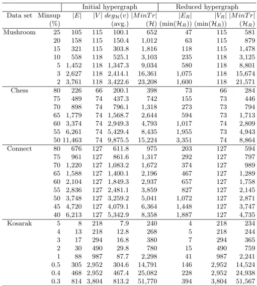
Hypergraph Reduction. Table 3 presents the hypergraphs and the transver-sals computed by F IBAD. Let us recall that for an experiment (a data set and a minsup value) the computed hypergraph, noted H = (V , E), correspond to the complement of the itemsets of the positive border (V ⊆ I and E = Bd+(S)). The reduced hypergraph of H, noted HR, is computed with Algorithm 2 (HR = HR(H)). For each data sets and minsup values, we have the number of hy-peredges of H (|E|), the number of vertices of H (|V |), the average degree of a vertex (degH(v)), the number of minimal transversals of H (|M inT r(H)|), the number of hyperedges of min(HR) (|ER|), the number of vertices of min(HR) (|VR|) and the number of minimal tranversals of HR (|M inT r(HR|). In order to better show the impact of the reduction, we consider here min(HR) instead of HR. The computation of min(HR) has no consequences on the computation of minimal transversals (see Proposition 1).
We can observe that the generated hypergraphs H strongly intersect, i.e., the average degree of a vertex is close to the number of hyperedges. These results confirm the observation made at the beginning of Sect. 5.
The number of vertices is almost the same in the initial hypergraph and the reduced hypergraph. The number of hyperedges of the reduced hypergraph is much lower than the number of hyperedges of the initial hypergraph. For in-stance, on Chess with minsup equals to 50%, there are 3,351 hyperedges instead of 11,463. The ”space savings” (i.e., 1 −|ER|
|E| ) is equal to 70.7%. In average, over all the data sets, the space savings is equal to 63%.
We can also see that, in general, the number of minimal transversals of the re-duced hypergraph is lower than the number of minimal transversals of the initial
Table 3. Computed hypergraphs and transversals.
Initial hypergraph Reduced hypergraph Data set Minsup |E| |V | degH(v) |M inT r| |ER| |VR| |M inT r|
(%) (avg.) (H) (min(HR)) (min(HR)) (HR)
Mushroom 25 105 115 100.1 652 47 115 581 20 158 115 150.4 1,012 63 115 879 15 321 115 303.8 1,816 118 115 1,478 10 558 118 525.1 3,103 235 118 3,125 5 1,452 118 1,347.3 9,034 580 118 8,801 3 2,627 118 2,414.1 16,361 1,075 118 15,674 2 3,761 118 3,422.6 23,208 1,600 118 21,571 Chess 80 226 66 200.1 398 73 66 284 75 489 74 437.3 742 155 73 446 70 898 74 796.1 1,318 273 73 794 65 1,779 74 1,568.7 2,644 594 73 1,713 60 3,374 74 2,949.3 4,793 1,017 74 2,809 55 6,261 74 5,429.4 8,435 1,955 73 4,943 50 11,463 74 9,875.5 15,224 3,351 74 8,864 Connect 80 676 127 611.8 975 203 127 594 75 961 127 861.6 1,317 292 127 797 70 1,220 127 1,083.2 1,672 374 127 989 65 1,588 127 1,400.1 2,196 467 127 1,289 60 2,104 127 1,849.3 2,937 657 127 1,758 55 2,836 127 2,481.1 3,859 827 127 2,145 50 3,748 127 3,259.2 5,041 1,072 127 2,871 45 4,720 127 4,079.1 6,364 1,448 127 3,747 40 6,213 127 5,342.9 8,358 1,887 127 4,735 Kosarak 5 8 218 7.9 240 4 218 234 4 13 218 12.8 268 5 218 244 3 17 294 16.8 380 7 294 365 2 30 490 29.8 780 15 490 759 1 88 987 87.7 2,298 41 987 2,241 0.5 305 2,952 304.6 14,791 146 2,952 14,524 0.4 468 2,952 467.4 25,082 228 2,952 24,938 0.3 814 3,804 813.2 51,770 394 3,804 51,567
hypergraph. This is not always true. For instance, on Mushroom with minsup equals to 10%, there are 3,103 minimal transversals for H and 3,125 for HR. Let us take an example to illustrate this point. The minimal transversals of the hypergraph {ABC, ABD, ABE, ABF, ABG} are {A, B, CDEF G}. There are 3 minimal transversals. Now, let us consider the hypergraph {AC, ABD, BG}, there are 4 minimal transversals ({AB, AG, BC, CDG}).
The hypergraph reduction is efficient in view of the space saving. Let us recall, that the hyperedges of the reduced hypergraph are selected using a heuristic which favors the search of approximate minimal transversals (see Sect. 5). Thus, our algorithm reduces the hypergraph while keeping the most important parts to find approximate minimal transversals.
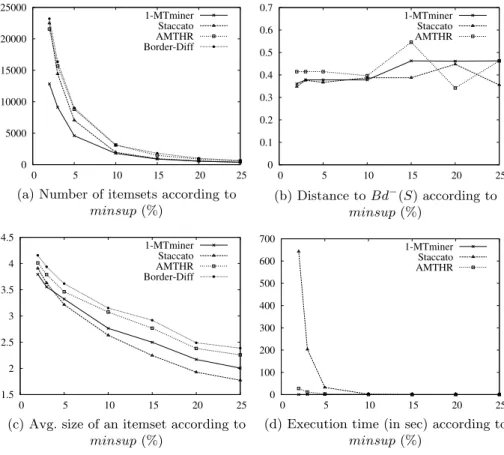
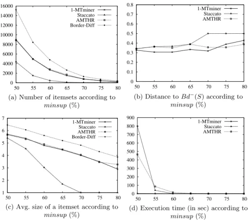
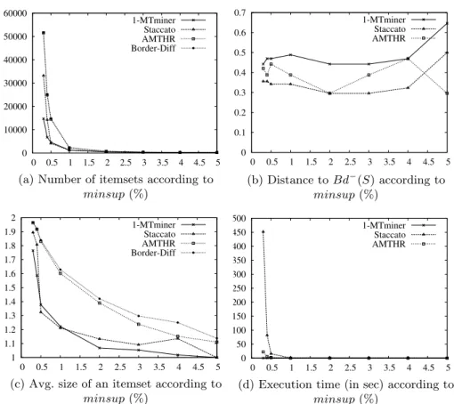
Approximate Negative Borders. Figures 3, 4, 5 and 6 present, for each data sets, (a) the number of itemsets of the computed negative borders, (b) the distance between the computed negative borders and the exact negative borders, (c) the average size of an itemset of the computed negative borders, and (d) the execution time, according to the minsup value.
We can observe that the cardinality ofBdg−(S) is lower than the cardinality of Bd−(S) for each data sets. The itemsets of Bdg−(S) are shorter than the itemsets of Bd−(S). On Mushroom and Kosarak, the cardinality of Bdg−(S) produced by AM T HR is very close to the cardinality of Bd−(S). The generated itemsets with AM T HR are a little shorter than the itemsets of the exact borders. For 1-M T miner, the cardinality of Bdg−(S) is the smallest on Mushroom and Kosarak. Staccato has generated the shortest itemsets on Mushroom but they are numerous. The itemsets produced by 1-M T miner and Staccato are very short on Kosarak. On Chess and Connect, AM T HR and 1-M T miner have produced a similar number of itemsets. These itemsets have a very close average size. We can remark that Staccato has produced a very small number of itemsets, and the average size of the itemsets is very small, on Chess and Connect.
Regarding the distance (between Bdg−(S) and Bd−(S)), AM T HR is not the best but it is close to the best algorithm for each data sets. Staccato has obtained the closest borders on Mushroom and Kosarak. This can be explained by the fact that λ has been set to high values for these data sets. This was not possible for Chess and Connect (dense data sets) and this explains why Staccato has the worst results on these data sets. 1-M T miner has produced the closest borders on Chess and Connect. These data sets are dense and they have many long itemsets in the positive borders (see Sect. 6.1). Let us remember that δ-M T miner produces δ-minimal transversals: minimal transversals which can miss at most δ hyperedges (see Sect. 3). δ-M T miner does not control where are the missed hyperedges. On dense data sets, this is not a problem because the possibilities to miss a hyperedge are few many. Let us also note that δ-M T miner is particularly fast on dense data sets.
Concerning the execution time to compute the approximate negative borders, Staccato is the slowest and 1-M T miner is the fastest. AM T HR is relatively fast on Mushroom and Kosarak but not on Chess and Connect.
We can conclude that Staccato and 1-M T miner are the best to compute g
Bd−(S) respectively on sparse and dense data sets. Nevertheless, AM T HR is close to the best algorithm for each data sets. We can also note that AM T HR is not sensitive to the type of data sets, contrary to the other algorithms. Only the execution time varies (it is higher on dense data sets).
Approximate Positive Borders. Figures 7, 8, 9 and 10 present, for each data sets, (a) the number of itemsets of the computed positive borders, (b) the distance between the computed positive borders and the exact positive borders, (c) the average size of an itemset of the computed positive borders, and (d) the execution time, according to the minsup value.
The number of itemsets ofBdg+(S) with AM T HR is the lowest on Mush-room. On the other data sets, Staccato has generated the lowest number of itemsets. 1-M T miner have produced more itemsets than AM T HR, except for Kosarak. The itemsets ofBdg+(S) are longer than the itemsets of Bd+(S). They are the longest with Staccato or AM T HR on each data sets.
AM T HR has obtained the closestBdg+(S) to Bd+(S) on all the data sets. On Connect, 1-M T miner has also obtained good results. On Kosarak, Staccato and 1-M T miner have produced bad results. This can be explained by the small number of itemsets of Bdg−(S) and these itemsets are too short. The transition toBdg+(S) produces too few itemsets and these itemsets are too long. The other bad results can be explained by the same remark.
The itemsets ofBdg+(S) are longer than the itemsets of Bd+(S) and AM T HR has obtained low distance values. We can say that the approximate positive bor-ders generated by AM T HR contain some itemsets with new items, while being close to the itemsets of the exact positive border. These new items could be interesting for some applications like document recommendation.
Regarding the execution time, on Mushroom, Chess and Connect, 1-M T miner is the slowest and Staccato is the fastest. On Kosarak, 1-M T miner is the fastest and Staccato is the slowest. The execution time of AM T HR is not the best but still correct.
We can conclude that AM T HR is the best to compute Bdg+(S). The dis-tances are the lowest, the number is reduced, and the execution time is correct. We explain these results by the characteristics ofBdg−(S) produced by AM T HR. We have previously seen that the cardinality ofBdg−(S) is a little lower than the cardinality of Bd−(S), and the itemsets ofBdg−(S) are a little shorter than the itemsets of Bd−(S). The transition to Bdg+(S) produces some itemsets longer than the itemsets of Bd+(S) while being close to Bd+(S). The other algorithms have not done that.
Table 4. Global results obtained on all the computed approximate borders. Method Avg. distance Avg. number of itemsets Avg. time (sec.)
AM T HR 0.323 3342.6 15.05
1-M T miner 0.384 2191.1 1.53
Staccato 0.452 1989.4 41.63
Border-Dif f - 4492.1 28.88
Global results. Table 4 presents the average distance, the average number of itemsets, and the average execution time over all the computed borders of all the data sets. The results obtained by the computation of the exact borders by dualization using Border-Dif f , are presented at the last line of the table.
0 5000 10000 15000 20000 25000 0 5 10 15 20 25 #itemsets minsup 1-MTminer Staccato AMTHR Border-Diff
(a) Number of itemsets according to minsup (%) 1.5 2 2.5 3 3.5 4 4.5 0 5 10 15 20 25
Avg. size of an itemset
minsup
1-MTminer Staccato AMTHR Border-Diff
(c) Avg. size of an itemset according to minsup (%) 0 0.1 0.2 0.3 0.4 0.5 0.6 0.7 0 5 10 15 20 25 Distance minsup 1-MTminer Staccato AMTHR (b) Distance to Bd−(S) according to minsup (%) 0 100 200 300 400 500 600 700 0 5 10 15 20 25 Time (s) minsup 1-MTminer Staccato AMTHR
(d) Execution time (in sec) according to minsup (%)
Fig. 3. Negative borders computed on Mushroom
We can observe that AM T HR has obtained the lowest average distance, and an average number of itemsets smaller than the average number of itemsets of the exact borders. The average execution time is correct. We can conclude that AM T HR is the best of the used methods in overall. Moreover, we have observed that AM T HR is robust according to the different types of data sets, contrary to 1-M T miner which fails on sparse data sets and Staccato which does not produce good results on dense data sets. Let us remark that we have used Border-Dif f to compute the exact minimal transversals of the reduced hypergraph (Step 3 of Algorithm 1). We have also used it for the computation of the approximate positive border (Step 4 of Algorithm 1). This is possible to use another more efficient algorithm, for instance one of the two algorithms presented in [32], in order to decrease the execution time.
FIBAD vs. CartesianContour. Table 5 presents the average distance, the average number of itemsets, and the average execution time over several approx-imate positive borders computed by F IBAD and CartesianContour. Indeed,
0 2000 4000 6000 8000 10000 12000 14000 16000 50 55 60 65 70 75 80 #itemsets minsup 1-MTminer Staccato AMTHR Border-Diff
(a) Number of itemsets according to minsup (%) 1 2 3 4 5 6 7 50 55 60 65 70 75 80
Avg. size of an itemset
minsup
1-MTminer Staccato AMTHR Border-Diff
(c) Avg. size of a itemset according to minsup (%) 0 0.1 0.2 0.3 0.4 0.5 0.6 0.7 0.8 50 55 60 65 70 75 80 Distance minsup 1-MTminer Staccato AMTHR (b) Distance to Bd−(S) according to minsup (%) 0 100 200 300 400 500 600 700 800 900 50 55 60 65 70 75 80 Time (s) minsup 1-MTminer Staccato AMTHR
(d) Execution time (in sec) according to minsup (%)
Fig. 4. Negative borders computed on Chess Table 5. F IBAD vs. CartesianContour.
Approach Avg. distance Avg. number of itemsets Avg. time (sec.)
F IBAD 0.289 286.6 9.67
CartesianContour 0.283 606.2 49.31
CartesianContour has not been able to compute the approximate positive bor-ders on Chess (minsup < 70%), Connect (minsup < 75%) and Kosarak (minsup < 1%). 17 of the 31 positive borders have been computed. Thus, the values presented in Table 5 have been computed only on these borders. This is why CartesianContour is not present in the previous results and discussion.
We observe that the average distances are very close. Nevertheless, the av-erage number of itemsets of the approximate positive borders is the lowest with F IBAD (for information, there are 728.7 itemsets in average in the 17 exact positive borders). We also see that F IBAD is faster than CartesianContour. We can conclude that F IBAD is better than CartesianContour to generate
0 1000 2000 3000 4000 5000 6000 7000 8000 9000 40 45 50 55 60 65 70 75 80 #itemsets minsup 1-MTminer Staccato AMTHR Border-Diff
(a) Number of itemsets according to minsup (%) 1 1.5 2 2.5 3 3.5 4 4.5 5 5.5 6 40 45 50 55 60 65 70 75 80
Avg. size of an itemset
minsup
1-MTminer Staccato AMTHR Border-Diff
(c) Avg. size of an itemset according to minsup (%) 0 0.1 0.2 0.3 0.4 0.5 0.6 0.7 0.8 40 45 50 55 60 65 70 75 80 Distance minsup 1-MTminer Staccato AMTHR (b) Distance to Bd−(S) according to minsup (%) 0 20 40 60 80 100 120 40 45 50 55 60 65 70 75 80 Time (s) minsup 1-MTminer Staccato AMTHR
(d) Execution time (in sec) according to minsup (%)
Fig. 5. Negative borders computed on Connect
approximate positive borders. Moreover, CartesianContour has some problems with dense data sets, and the minsup value can not be low.
7
Conclusion
This paper deals with the problem of approximate borders computed by dual-ization. At the same time, this is a challenging theoretical problem which may play a valuable role in a wide range of applications. To achieve this goal, we introduced here the F IBAD approach leveraging dualization and computation of approximate minimal transversals of hypergraphs. Its originality comes from a new function we have defined to compute approximate negative borders. For this purpose, we start by reducing the initial hypergraph and, then, we compute its exact minimal transversals. This processing is implemented by the function AM T HR and used by F IBAD as an approximate dualization. To evaluate our approximate dualization method, we replaced AM T HR with other methods that compute approximate minimal transversals. In particular, we considered
0 10000 20000 30000 40000 50000 60000 0 0.5 1 1.5 2 2.5 3 3.5 4 4.5 5 #itemsets minsup 1-MTminer Staccato AMTHR Border-Diff
(a) Number of itemsets according to minsup (%) 1 1.1 1.2 1.3 1.4 1.5 1.6 1.7 1.8 1.9 2 0 0.5 1 1.5 2 2.5 3 3.5 4 4.5 5
Avg. size of an itemset
minsup
1-MTminer Staccato AMTHR Border-Diff
(c) Avg. size of an itemset according to minsup (%) 0 0.1 0.2 0.3 0.4 0.5 0.6 0.7 0 0.5 1 1.5 2 2.5 3 3.5 4 4.5 5 Distance minsup 1-MTminer Staccato AMTHR (b) Distance to Bd−(S) according to minsup (%) 0 50 100 150 200 250 300 350 400 450 500 0 0.5 1 1.5 2 2.5 3 3.5 4 4.5 5 Time (s) minsup 1-MTminer Staccato AMTHR
(d) Execution time (in sec) according to minsup (%)
Fig. 6. Negative borders computed on Kosarak
two alternative methods based on the δ-M T miner and Staccato algorithms, respectively. We also compared our method with CartesianContour that com-putes directly, without dualization, the approximate borders. The experimental results have showed that our method outperforms the other methods as it pro-duces borders which have the highest quality. It propro-duces an approximate posi-tive border smaller than the exact posiposi-tive border, while keeping a low distance with the exact border. Through these experiments, we have observed that our approach is robust according to the different types of data sets. We can note that for sparse data sets, it is particularly efficient. This point is very interesting for future applications on the Web where most of the constructed data sets are sparse and very large (for instance, data from a web server log file). We have also seen that the proposed approach is able to find potentially interesting items for some applications like document recommendation, for instance. In the future, we will develop a recommendation system using the approximate positive borders generated by F IBAD. In that way, we will able to evaluate the quality of the generated borders in an applicative context.
0 500 1000 1500 2000 2500 3000 3500 4000 0 5 10 15 20 25 #itemsets minsup 1-MTminer Staccato AMTHR Border-Diff
(a) Number of itemsets according to minsup (%) 6 7 8 9 10 11 12 13 0 5 10 15 20 25
Avg. size of an itemset
minsup
1-MTminer Staccato AMTHR Border-Diff
(c) Avg. size of an itemset according to minsup (%) 0 0.1 0.2 0.3 0.4 0.5 0.6 0.7 0 5 10 15 20 25 Distance minsup 1-MTminer Staccato AMTHR (b) Distance to Bd+(S) according to minsup (%) 0 5 10 15 20 25 30 35 40 0 5 10 15 20 25 Time (s) minsup 1-MTminer Staccato AMTHR
(d) Execution time (in sec) according to minsup (%)
0 2000 4000 6000 8000 10000 12000 50 55 60 65 70 75 80 #itemsets minsup 1-MTminer Staccato AMTHR Border-Diff
(a) Number of itemsets according to minsup (%) 6 8 10 12 14 16 18 20 22 24 50 55 60 65 70 75 80
Avg. size of an itemset
minsup
1-MTminer Staccato AMTHR Border-Diff
(c) Avg. size of an itemset according to minsup (%) 0 0.1 0.2 0.3 0.4 0.5 0.6 0.7 0.8 0.9 50 55 60 65 70 75 80 Distance minsup 1-MTminer Staccato AMTHR (b) Distance to Bd+(S) according to minsup (%) 0 2 4 6 8 10 12 50 55 60 65 70 75 80 Time (s) minsup 1-MTminer Staccato AMTHR
(d) Execution time (in sec) according to minsup (%)
0 1000 2000 3000 4000 5000 6000 7000 40 45 50 55 60 65 70 75 80 #itemsets minsup 1-MTminer Staccato AMTHR Border-Diff
(a) Number of itemsets according to minsup (%) 10 15 20 25 30 35 40 40 45 50 55 60 65 70 75 80
Avg. size of an itemset
minsup
1-MTminer Staccato AMTHR Border-Diff
(c) Avg. size of an itemset according to minsup (%) 0 0.1 0.2 0.3 0.4 0.5 0.6 0.7 40 45 50 55 60 65 70 75 80 Distance minsup 1-MTminer Staccato AMTHR (b) Distance to Bd+(S) according to minsup (%) 0 1 2 3 4 5 6 7 40 45 50 55 60 65 70 75 80 Time (s) minsup 1-MTminer Staccato AMTHR
(d) Execution time (in sec) according to minsup (%)
0 100 200 300 400 500 600 700 800 900 0 0.5 1 1.5 2 2.5 3 3.5 4 4.5 5 #itemsets minsup 1-MTminer Staccato AMTHR Border-Diff
(a) Number of itemsets according to minsup (%) 2 4 6 8 10 12 14 16 18 0 0.5 1 1.5 2 2.5 3 3.5 4 4.5 5
Avg. size of an itemset
minsup
1-MTminer Staccato AMTHR Border-Diff
(c) Avg. size of an itemset according to minsup (%) 0 0.1 0.2 0.3 0.4 0.5 0.6 0.7 0.8 0.9 0 0.5 1 1.5 2 2.5 3 3.5 4 4.5 5 Distance minsup 1-MTminer Staccato AMTHR (b) Distance to Bd+(S) according to minsup (%) 0 2 4 6 8 10 12 14 16 0 0.5 1 1.5 2 2.5 3 3.5 4 4.5 5 Time (s) minsup 1-MTminer Staccato AMTHR
(d) Execution time (in sec) according to minsup (%)
Fig. 10. Positive borders computed on Kosarak
References
1. Abreu, R., van Gemund, A.: A Low-Cost Approximate Minimal Hitting Set Al-gorithm and its Application to Model-Based Diagnosis. In: Proc. 8h Symposium on Abstraction, Reformulation and Approximation (SARA’09). Lake Arrowhead, CA, USA (July 2009)
2. Afrati, F., Gionis, A., Mannila, H.: Approximating a Collection of Frequent Sets. In: Proc. 10th ACM SIGKDD International Conference on Knowledge Discovery and Data mining. pp. 12–19. Seattle, WA, USA (August 2004)
3. Agrawal, R., Imielinski, T., Swami, A.: Mining Association Rules between Sets of Items in Large Database. ACM SIGMOD International Conference on Management of Data pp. 207–216 (May 1993)
4. Bailey, J., Manoukian, T., Ramamohanarao, K.: A Fast Algorithm for Computing Hypergraph Transversals and its Application in Mining Emerging Patterns. In: Proc. 3rd IEEE International Conference on Data Mining (ICDM’03). pp. 485– 488. Melbourne, Florida, USA (November 2003)
5. Bayardo, R.: Efficiently Mining Long Patterns From Databases. In: Proceedings of the ACM SIGMOD International Conference on Management of Data. pp. 85–93. Seattle (June 1998)
6. Berge, C.: Hypergraphs : Combinatorics of Finite Sets, vol. 45. North Holland Mathematical Library (1989)
7. Boley, M.: On Approximating Minimum Infrequent and Maximum Frequent Sets. In: Proc. 10th International Conference on Discovery Science (DS’07). pp. 68–77. Sendai, Japan (October 2007)
8. Boulicaut, J.F., Bykowski, A., Rigotti, R.: Free-sets : a Condensed Representation of Boolean Data for the Approximation of Frequency Queries. Data Mining and Knowledge Discovery 7(1), 5–22 (2003)
9. Burdick, D., Calimlim, M., Gehrke, J.: MAFIA: A Maximal Frequent Itemset Al-gorithm for Transactional Databases. In: Proc. International Conference on Data Engineering (ICDE’01). pp. 443–452. Heidelberg, Germany (2001)
10. De Marchi, F., Petit, J.: Zigzag: a new algorithm for mining large inclusion depen-dencies in database. In: Proc. 3rd IEEE International Conference on Data Mining (ICDM’03). pp. 27–34. Melbourne, Florida, USA (November 2003)
11. Dong, G., Li, J.: Efficient Mining of Emerging Patterns: Discovering Trends and Differences. In: Proc. 5th ACM SIGKDD International Conference on Knowledge Discovery and Data Mining Knowledge Discovery and Data Mining (SIGKDD’99). pp. 43–52. San Diego, USA (August 1999)
12. Dong, G., Li, J.: Mining Border Descriptions of Emerging Patterns from Dataset-Pairs. Knowledge and Information Systems 8(2), 178–202 (2005)
13. Ducournau, A., Bretto, A., Rital, S., Laget, B.: A Reductive Approach to Hy-pergraph Clustering: An Application to Image Segmentation. Pattern Recognition 45(7), 2788–2803 (2012)
14. Durand, N., Cr´emilleux, B.: ECCLAT: a New Approach of Clusters Discovery in Categorical Data. In: Proc. 22nd SGAI International Conference on Knowledge Based Systems and Applied Artificial Intelligence (ES’02). pp. 177–190. Cam-bridge, UK (December 2002)
15. Durand, N., Quafafou, M.: Approximation of Frequent Itemset Border by Comput-ing Approximate Minimal Hypergraph Transversals. In: Proc. 16th International Conference on Data Warehousing and Knowledge Discovery (DaWak’14). pp. 357– 368. Munich, Germany (September 2014)
16. Eiter, T., Gottlob, G.: Hypergraph Transversal Computation and Related Prob-lems in Logic and AI. In: Proc. 8th European Conference on Logics in Artificial Intelligence (JELIA’02). pp. 549–564 (2002)
17. Flouvat, F., De Marchi, F., Petit, J.M.: A new classification of datasets for frequent itemsets. Intelligent Information Systems 34, 1–19 (2010)
18. Flouvat, F., De Marchi, F., Petit, J.: ABS: Adaptive Borders Search of frequent itemsets. In: Proc. IEEE ICDM Workshop on Frequent Itemset Mining Implemen-tations (FIMI’04). Brighton, UK (November 2004)
19. Fredman, M.L., Khachiyan, L.: On the Complexity of Dualization of Monotone Disjunctive Normal Forms. Algorithms 21(3), 618–628 (1996)
20. Gouda, K., Zaki, M.J.: GenMax: An Efficient Algorithm for Mining Maximal Fre-quent Itemsets. Data Mining and Knowledge Discovery 11, 1–20 (2005)
21. Gunopulos, D., Khardon, R., Mannila, H., Saluja, S., Toivonen, H., Sharma, R.S.: Discovering All Most Specific Sentences. ACM Transactions on Database Systems 28(2), 140–174 (2003)
22. Han, J., Cheng, H., Xin, D., Yan, X.: Frequent pattern mining: current status and future directions. Data Mining and Knowledge Discovery 15, 55–86 (2007) 23. Hasan, M., Zaki, M.J.: MUSK: Uniform Sampling of k Maximal Patterns. In: SIAM
24. H´ebert, C., Bretto, A., Cr´emilleux, B.: A data mining formalization to improve hypergraph transversal computation. Fundamenta Informaticae, IOS Press 80(4), 415–433 (2007)
25. Jin, R., Xiang, Y., Liu, L.: Cartesian Contour: a Concise Representation for a Collection of Frequent Sets. In: Proc. 15th International Conference on Knowledge Discovery and Data Mining (KDD’09). pp. 417–425. Paris, France (June 2009) 26. Karonski, M., Palka, Z.: One standard Marczewski-Steinhaus outdistances between
hypergraphs. Zastosowania Matematyki Applicationes Mathematicae 16(1), 47–57 (1977)
27. Karypis, G., Aggarwal, R., Kumar, V., Shekhar, S.: Multilevel Hypergraph Par-titioning: Applications in VLSI Domain. IEEE Transactions on Very Large Scale Integration (VLSI) Systems 7(1), 69–79 (1999)
28. Kavvadias, D., Stavropoulos, E.: An Efficient Algorithm for the Transversal Hy-pergraph Generation. Graph Algorithms and Applications 9(2), 239–264 (2005) 29. Lin, D.I., Kedem, Z.M.: Pincer-Search: A New Algorithm for Discovering the
Max-imum Frequent Sets. In: Proc. International Conference on Extending Database Technology (EDBT’98). pp. 105–119. Valencia, Spain (1998)
30. Mannila, H., Toivonen, H.: Levelwise Search and Borders of Theories in Knowledge Discovery. Data Mining and Knowledge Discovery 1(3), 241–258 (1997)
31. Moens, S., Goethals, B.: Randomly Sampling Maximal Itemsets. In: Proc. ACM SIGKDD Workshop on Interactive Data Exploration and Analytics (IDEA’13). pp. 79–86. Chicago, Illinois, USA (2013)
32. Murakami, K., Uno, T.: Efficient Algorithms for Dualizing Large-Scale Hyper-graphs. Discrete Applied Mathematics 170, 83–94 (2014)
33. Pasquier, N., Bastide, Y., Taouil, R., Lakhal, L.: Efficient Mining of Association Rules Using Closed Itemset Lattices. Information Systems 24(1), 25–46, Elsevier (1999)
34. Ramamohanarao, K., Bailey, J., Fan, H.: Efficient Mining of Contrast Patterns and Their Applications to Classification. In: Proc. 3rd International Conference on Intelligent Sensing and Information Processing (ICISIP’05). pp. 39–47. Bangalore, India (December 2005)
35. Rioult, F., Zanuttini, B., Cr´emilleux, B.: Nonredundant Generalized Rules and Their Impact in Classification. Advances in Intelligent Information Systems, Series: Studies in Computational Intelligence 265, 3–25 (2010)
36. Ruchkys, D.P., Song, S.W.: A Parallel Approximation Hitting Set Algorithm for Gene Expression Analysis. In: Proc. 14th Symposium on Computer Architecture and High Performance Computing (SBAC-PAD’02). pp. 75–81. Washington, DC, USA (October 2002)
37. Satoh, K., Uno, T.: Enumerating Maximal Frequent Sets Using Irredundant Du-alization. In: Proc. 6th International Conference on Discovery Science (DS 2003). pp. 256–268. Sapporo, Japan (October 2003)
38. Vinterbo, S., Øhrn, A.: Minimal Approximate Hitting Sets and Rule Templates. Approximate Reasoning 25, 123–143 (2000)
39. Vreeken, J., van Leeuwen, M., Siebes, A.: Krimp: Mining Itemsets that Compress. Data Mining and Knowledge Discovery 23(1) (2011)
40. Yang, G.: The Complexity of Mining Maximal Frequent Itemsets and Maximal Frequent Patterns. In: Proc. International Conference on Knowledge Discovery in Databases (KDD’04). pp. 344–353. Seattle, WA, USA (2004)
41. Zhu, F., Yan, X., Han, J., Yu, P.S., Cheng, H.: Mining Colossal Frequent Pat-terns by Core Pattern Fusion. In: Proc. 23rd International Conference on Data Engineering (ICDE’07). pp. 706–715. Istanbul, Turkey (April 2007)