HAL Id: hal-01823765
https://hal-amu.archives-ouvertes.fr/hal-01823765
Submitted on 26 Jun 2018
HAL is a multi-disciplinary open access
archive for the deposit and dissemination of
sci-entific research documents, whether they are
pub-lished or not. The documents may come from
teaching and research institutions in France or
abroad, or from public or private research centers.
L’archive ouverte pluridisciplinaire HAL, est
destinée au dépôt et à la diffusion de documents
scientifiques de niveau recherche, publiés ou non,
émanant des établissements d’enseignement et de
recherche français ou étrangers, des laboratoires
publics ou privés.
To cite this version:
Bernard Xerri, Jean-François Cavassilas, Bruno Borloz. Passive Tracking in Underwater
Acous-tics. Signal Processing, Elsevier, 2002, 82 (8), pp.1067-1085. �10.1016/S0165-1684(02)00240-2�.
�hal-01823765�
Passive Tracking in Underwater Acoustics
Bernard Xerri*, Jean-François Cavassilas , Bruno BorlozSIS/GESSY, ISITV, av. G. Pompidou, BP 56,
83162 La Valette du Var Cedex, France
___________________________________________________________________________________________________ Abstract
This paper provides a novel passive underwater acoustic method to track a moving object called source or target, with the following constraints: the sensors location is fixed and imposed, and classical array processing techniques cannot be applied. The method proposed has been successfully used to track a surface vessel (2D problem) or an underwater target (3D problem). All the results presented have been obtained with real signals. The localization of the target requires the estimation of propagation delays, that means the duration between the instant of the signal emission and its reception on each receiver. The cross-correlation function is a suitable tool when the target is motionless, but needs to be extended to the ambiguity function when it is moving. The signal to noise ratio, the uniformity of power spectral density and the integration time are determining factors for the accuracy of the localization. We show that a whitening method and a Doppler compen-sation are necessary, and we propose a way to eliminate the significant problem of the reflected signals. Furthermore, a new configuration of the receivers is proposed, based on the idea of coupling receivers whose distance is chosen from experi-ment derived results. Furthermore, the algorithm proposed is susceptible to parallel impleexperi-mentation, thereby facilitating real-time uses. Experimental results with real time domain data are presented and compared to trajectories obtained by an active method.
Résumé
Cet article présente une nouvelle méthode d’écoute passive destinée à trajectographier un objet en mouvement appelé la “source” ou la “cible”, avec les contraintes suivantes : le réseau de capteurs est fixe et imposé, et les méthodes classiques de traitement d’antenne ne peuvent pas s’appliquer. La méthode proposée ici a été utilisée avec succès pour trajectographier un bâtiment de surface (problème à deux dimensions) ou une cible sous-marine (problème à trois dimensions). Tous les résultats présentés ont été obtenus sur des signaux réels. Le calcul de la position de la cible nécessite l’estimation des temps de propagation, c’est-à-dire du temps écoulé entre l’instant d’émission du signal et sa réception sur chaque capteur. La fonction d’intercorrélation est un outil opportun lorsque la cible est immobile mais elle doit être étendue à la notion d’ambiguïté quand la source est en mouvement. Le rapport signal à bruit, l’uniformité de la densité spectrale de puissance et la durée d’intégration sont des facteurs déterminants pour la précision de la localisation. Nous montrons qu’une méthode de blanchiment et une compensation de l’effet Doppler sont nécessaires et nous proposons un moyen d’éliminer le prob-lème des trajets multiples. Par ailleurs, une nouvelle configuration des capteurs est proposée, fondée sur l’idée d’associer des hydrophones séparés d’une distance déterminée de manière expérimentale. Des résultats de trajectographies sont pré-sentés et comparés aux trajectoires obtenues par une méthode active.
Keywords: source localization ; passive listening ; tracking ; cross-ambiguity function ; Doppler ; whitening ; propagation delays estimation ; AR models ; lattice filter
___________________________________________________________________________
Notations
M(t) position of the target at time t v
→
(t) speed of the target at time t
→
(t) acceleration of the target at time t S(t) signal emitted by the target at time t Hi hydrophone number i
N number of hydrophones
Np number of pairs of hydrophones for the short base-line system
Si(t) signal received on Hi at time t
HiM(t) distance between Hi and M at time t
c velocity of sound in the sea
tpi(t) propagation duration between the source and Hi
Bi(t) noise measured on Hi at time t
ij(t) differential time delay between the receptions on Hi
and Hj at time t
SS() correlation function of a stationary signal S(t) ij(t1,t2) cross-correlation function of Si(t) and Sj(t)
frequency (Hz)
Cij() coherence function of Si(t) and Sj(t)
ij() cross-spectral density function of Si(t) and Sj(t)
E[ ] expected value of [ ]
T integration time length of S(t) B upper bound frequency of S(t)
Di(t) 1st-order Doppler coefficient related to Hi at time t DDi(t) 2nd-order Doppler coefficient related to Hi at time t Dji(t) 1st-order differential Doppler coefficient related to
the jth and the ith receivers at time t.
DDji(t) 2nd-order differential Doppler coefficient related to
the jth and the ith receivers at time t. fog(x) = f(g(x))
te emission time of S
SNR signal to noise ratio
1. Introduction
Underwater acoustic tracking using passive sensors has been extensively studied, and source localization continues to be a main area of interest in ocean acoustics. Although, the approach presented in this paper is innovative.
This paper addresses the problem of tracking a surface or underwater moving target from its radiated noises received on fixed and geographically separated hydrophones [1][13]. The available sensors do not form an array as commonly accepted. Therefore, as we are in a near field configuration, the propagation duration which is the time elapsed between the time a signal is emitted and the time it is received by a sensor is finite and cannot be ignored. Our paper deals explic-itly with the propagation delays which are time varying and with the resulting Doppler effect.
Initially, the receivers field was used to perform active tracking of surface vessels equipped with transmitters. Of course, such a method is no more feasible in the case of fast maneuvering underwater sources. Then, it was natural to im-plement a passive method as a comim-plement to the active one. Active methods can be separated into several techniques : the targets to track can be equipped with a transmitter [11][18][21]. Then, the emitted signal is known, and array processing techniques, with linear or nonlinear arrays, are generally used. But such methods require the installation of
powerful and expensive transmitters on objects to track, dis-turbing electronic systems on board and modifying hydrody-namic qualities of underwater targets. These disadvantages make unacceptable such a method for underwater targets. Without any transmitter, under the hypothesis of far field, linear array are used. The emitted signal is generally a known line spectrum signal (chirp, modulated or not) ; several ways are possible : short impulses which do not take into account the Doppler effect, long impulses for which the Doppler effect must be considered, or specific signals insensitive to Doppler effect [9][29]. The disadvantages of active methods are evident, especially for reasons of discretion, but in the absence of such restrictions, they are very useful, as for in-stance for communications between maneuvering autono-mous underwater vehicles [26].
However, our topic is not interested in active methods but in passive methods, and the results obtained with active methods are only used to verify those obtained with our method for surface targets.
Several passive methods have been developed. Array pro-cessing techniques are generally used to estimate the source azimuth; for narrow-band signals, the tracking of line spec-trum or more geometrical methods are used [23][24][25]. The receivers form antennae which are linear or nonlinear, mov-ing or fixed. For example, the use of sonobuyos equipped with GPS (global position system) receivers can be consid-ered for the detection of multiple impacts on the ocean sur-face [22]. In this case, however, the authors try to detect impulsive sources, not to track a moving vehicle ; in such a scheme, the Doppler effect is not taken into account.
Thus, short baseline systems and long baseline systems have been developed [27][29]. Our paper considers the case of fixed, imposed and nonlinear receivers, and mixes the two systems according to the phase (initialization or tracking).
Taking into account the characteristics of the available sensors, our problem is to develop a passive method to track a target which is emitting an unknown continuous broadband spectrum, with fixed and spatially distributed hydrophones. The hydrophone field is large enough to contain the whole path of the target.
The localization problem is solved by estimating the dif-ferent delays of reception between the receivers ; commonly, generalized correlation methods are used [2][4][9][10][17] [19]. There are at least two ways of obtaining the delays of reception between two receivers : time domain working methods are chosen to estimate them, even though a frequen-cy correction is performed to improve the result [5][16]. Such methods can also be applied in other domains like communi-cations between vehicles [28].
Because of the signal to noise ratio which is not always favourable, it is necessary, to evaluate the quantities of inter-est, to use an integration time which cannot be as small as possible [14][15]. Because the target is maneuvering and considering the unavoidably significant integration times, it is not possible to ignore the Doppler effect, and therefore a Doppler compensation is necessary. To enable robust com-munications between moving vehicles, such a compensation is usually achieved by multirate sampling and linear interpo-lation [26][28]. For a fast maneuvering target, a linear inter-polation is no more sufficient. A higher order compensation (parabolic or more) must be achieved.
In brief, a hydrophone field consisting of fixed sensors which are not aligned is used to track a fast moving object emitting an unknown broadband signal which might contain narrow-band components. Therefore, a long baseline system is imposed. The signal to noise ratio is unknown, but custom-arily lies between -20 and 40 dB.
The main problems are the necessity of a compensation of the Doppler effect and the presence of bottom bounces or surface-reflected paths of the emitted signal. A remedy to eliminate the reflected paths is proposed, based on lattice filters and a AR modelling [6][7][8][30]; this method has been successfully tested on real data. Note that a suitable processing of the reflected paths can contribute to additional information.
Considering the maneuverability of the target and the in-tegration time, a first-order or a second-order Doppler com-pensation is necessary.
As the domain of delays and Dopplers explored is large, it is necessary to consider a short baseline system which needs to be related to the long baseline system to realize a complete system.
The results obtained for surface vehicles with real data have been compared with those obtained with a radar. It is pivotal to note that the whole experimental results presented have been obtained with real data.
Furthermore, the implementation on a parallel architec-ture machine of the algorithm proposed has been performed, allowing a real-time calculation of the path.
This paper is organized as follows. Section 2 presents the experimental conditions and constraints ; convincing argu-ments are given for the choice of our method. Section 3 for-mulates a mathematical model and a method to track targets, using the existing ranges of hydrophones ; general and useful tools are introduced and adapted to the chosen method which is a long baseline method. Section 4 presents the practical method and tracking results ; after a critical analysis, a sec-ond method (short baseline) is proposed, requiring additional hydrophones whose position is chosen from experimental results. The both methods (long and short baselines) are mixed in a more general method. Section 5 is dedicated to the design of algorithms adapted to the new configuration of the hydrophones. Definitive results are presented in section 6, with the realization of a real-time tracking machine.
Finally, this study has been performed for the CEM (‘Centre d'Essais de la Méditerranée’ or ‘Mediterranean test range’) which owns three underwater ranges of hydrophones named Tremail.
2. Problem statement
The problem is formulated in the three dimensional case, and we assume that the source path owns straight lines and curve parts.
The Tremail ranges
Each of the three ranges owns fixed hydrophones whose positions are perfectly known. The field of interest is the shallow range called T.F.F. (“Tremail Faible Fond”) which contains 8 receivers located approximately 250 m under the sea surface and on average 400 m away from one another (cf. figure 11).
Each hydrophone is connected to a reception center which records and digitizes analog signals. The hydrophones of a range are not immersed exactly at the same depth ; that al-lows to address the 3D localization problem ; however, the precision in z coordinate (depth) will be lower than in other coordinates. The depth indicated above is a mean value ; a discrepancy of several tens of metres is possible.
The nature of noises and hydrophones characteristics
Radiated noises of ships and underwater targets can be divided [20] into mechanical noises (engine, propellers, vi-brations, …) and hydrodynamic noises (flow on the hull, air bubbles, cavitation,…). The former are quasi-periodic signals whereas the spectral representation of the latter is continuous. The hydrophones of the Tremail cannot detect very low fre-quency signals (their low cutting-off frefre-quency is 100 Hz) ; their high cutting-off frequency is 100 kHz.
The surrounding noise results from the addition of several noises the origins of which are various : noises due to sea state, biological noises, molecular turbulence… These noises are located in different spectral bands. Number of studies have classified them according to their importance and fre-quency.
For the following study, it is pivotal to note that, as many experiments proved, sea noises measured on two sensors of the Tremail are uncorrelated.
The interferometry method
Among the aforementioned methods which could be used for the localization of a maneuvering target, we choose the interferometry method.
In fact, an azimutal method would use the Tremail as an array and requires the observation of signals with very low frequencies, which is not compatible with the low cut-off frequency of the sensors. Concerning the method which con-sists in following the line spectrum shifted by the Doppler effect, it needs a precise knowledge of the emitted signal for every target ; in our case, this a priori information is not available.
Due to the characteristics of the hydrophones and because the emitted signal is unknown, the chosen method is the broadband interferometry which has the advantage of exploit-ing the broadband component of the emitted signal. What’s more, the main interest of this approach is that, as said be-fore, noises on two sensors of the Tremail are uncorrelated. Furthermore, the absolute power fluctuations are not taken into account by such a method. According to experimental data analysis, the sampling rate is 10 kHz for ships.
3. Statements related to tracking
The propagation model assumptions
The velocity of the sound in water c is supposed to be not affected by the medium considered homogeneous (c is con-stant). We note {M(te)} the trajectory of the target.
If S(te) is the signal emitted by the target, the signal re-ceived on Hi is
( )
(
)
( )
(
( )
)
i e pi e αi e i e pi e S t +t t = S t +B t +t t (1) where− tpi(te) is the propagation duration, i.e. the duration between
the emission time te of S(t) and the time it is received on
Hi. Because the target is moving, tpi depends on te, and
( )
i( )
e pi e H M t t t c = (2)− the coefficients i are introduced to respect the
conserva-tion of energy.
As mentioned above, the noises Bi are uncorrelated.
The remainder of the paper will ignore the coefficients i
because interferometry methods are not interested in absolute energy level. Calculated cross-correlations will be exact ex-cept for a multiplicative coefficient.
The localization problem
We do not know the different values tpi(te) ; so we have to
estimate them. From (2), we define the differential time delay between the arrivals on two hydrophones Hi and Hj by
ij
( )
e pj( )
e - pi( )
e = j( )
e i( )
e H M t H M t t t t t t c = − . (3)Such an equation represents an hyperboloid the focuses of which are Hi and Hj ; then, three equations are necessary to
know M(te) from the different ij(te). But the localization of
the target requires the knowledge of ij(te) for the same
emis-sion time te. Then one receiver must be taken as a reference
(this will be H1); the differential time delays can be written
( )
( )
( )
1j te =tpj te - tp1 et
.
For a fixed error on propagation delays, the accuracy of the localization is all the better as the distance between the receivers grows.
Time delay estimation classical methods for stationary signals
Two classes of estimators can be used, working in time or frequency domains, to estimate the differential delays 1i at
the same time te. They both use the fundamental properties of
the correlation function SS() of a stationary signal S(t) :
SS() is maximal for = 0.
The cross-correlation function of two signals received on the sensors Hi and Hj is
( )
( )
( ) ( )
i j 1 2, ij 1 2, i 1 j 2 S S t t t t S t S t
= =E . (4)
If the target and the receivers are fixed, our model leads to
(
)
(
) (
)
ij t t1 2, S t1 tpi S t2 tpj E − − ,
because noises on two sensors are uncorrelated.
If the emitted signal S(t) is stationary with a microscopic correlation, and power 2 then
(
)
( )
(
) (
)
2(
)
ij t t, τ ij τ S t tpi S t τ tpj δ τ τij + = E − + − = −which is maximum for = ij. The ij could also be found by
evaluating the slope of the phase of the cross-power spec-trum. More generally, it has been established that the estima-tion of ij is simply the abscissa value at which the
cross-correlation peaks [2]. However, the maximum likelihood optimal estimator of time delay is a 'filtered' cross-correlation
function called ‘generalized cross-correlation’ and written
( )
i j (g)
ij τ = P(ν) S S(ν) = P(ν) (ν)ij
F F ,
that is the Fourier Transform of the weighted cross-spectral density ij(). For P()= 1,
( )
(g) ij τ
is the common correlation function. Several weighting functions have been proposed [3][4] :
- PHAT (phase transform) :
ij 1 ( ) (ν) P = ,
- SCOT (Smoothed COher-ence Transform) : ii jj 1 ( ) = ( ) ( ) P , - HT (Hannan-Thomson) : ij ij ij ( ) 1 ( )= ( ) 1 ( ) C P C − , where ij ij ii jj ( ) ( ) ( ) ( ) C =
is the coherence function. The PHAT transformation enhances the spectral areas with a low signal to noise ratio, whilst the HT method en-hances the spectral rays reduced by the coherence function.
Hence, the choice of the SCOT method which leads to the coherence function whose properties are adapted to the inter-ferometry methods is natural [5]. Such a weighting whitens spectral areas where information is high ; the cross-correlation peak becomes more narrow, improving the esti-mation of time delay. What’s more, the phase of ij() is not
modified so that the abscissa value at which the cross-correlation peaks is not changed.
extension to the case of non-stationary signals Considering a zero mean non stationary signal S(t), we can also define a correlation range c such as
c( , τ) ( ) ( - τ) 0 | τ | τ
SS t S t S t
=E = .
If the stationarity fluctuations are small with respect to the duration c, then
(
, 0)
(
, τ)
, | τ | 0SS t SS t t
.
The following function
2 2 1 ξ(τ) ( , τ)d T T SS T − t t =
is also maximal for = 0. It is essential to note that this func-tion can be defined even for non stafunc-tionary signals, and that even though () is not representative of the signal character-istics, its maximum is all the same reached for = 0.
The choice of the integration time length T is delicate and must be made according to experimental analysis : it depends closely on the SNR : a low SNR requires to increase T, but in return, increasing T too much makes the Doppler effect prominent and involves expensive computations. Hence, for fast maneuvering targets, T cannot be chosen too large.
In the same way, we can define, using (4)
2 2 ij 1 ij ξ (τ) ( , τ)d T T T − t t =
. (5)It can be proved [1] that, as above,
(
ij)
ijargmax ( ) = . (6) In the particular case where S(t) is a stationary signal, SS(t,)
does not depend on t and
() = SS() or ij() = SS(−ij)
and the relation (6) is still true.
In this study emitted signals are non stationary and conse-quently ij() is used instead of ij(t,). What’s more, such a
quantity is suitable for the ergodicity assumption. We want to estimate ij and not statistical characteristics of the emitted
signal, thus the calculation of ij() is always suited to our
problem : it will allow to calculate delays even if the integrat-ed functions cannot be interpretintegrat-ed as correlation functions.
variance of the estimation of the differential delays The coherence function verifies the relation |Cij()| 1 ;
in the absence of noise, the equality is reached if the under-water medium behaves as a linear filter. Several factors con-tribute to coherence destruction
- a low SNR in a cross-spectral band,
- the medium does not behave as a linear filter,
- the existence of reflected signals with no perceptible re-duced power.
It has been established [4] that the variance of the error of estimation of ij is
(
)
(
)
2 2 ij 2 0 ij ij 2 2 2 ij 0 1 (ν) ν ν 1 ˆτ - τ = lim 8π | (ν)| ν ν B B B C d T C d → −
Ewhere B is the upper frequency bound of S(t), under the fol-lowing hypotheses
- the shift of the cross-correlation peak is due to the additive noises,
- T is large enough to ensure that, around the peak, the es-timated cross-correlation is identical to its second sum se-ries expansion,
- T is much larger than the signal correlation support, - Si and Sj are jointly gaussian.
So if Cij(ν)=d constant in the band [0,B],
(
)
2 2 ij ij 2 3 2 3 1 ˆτ - τ = 8π d TB d −
E .In the absence of noise, Si and Sj are coherent, and
(
)
2 ij ij ˆτ - τ = 0
E .The Doppler effect
The aforementioned reasons explain why the integration time T cannot be chosen as small as wanted. This constraint will induce a Doppler effect. What’s more, as the target is moving, tpi(te) changes with time. Such changes will lead to
modifications of the received signals which can be significant enough to make the cross-correlation peak undetectable. The
higher the speed and acceleration of the target are, the greater the deformation of the signal becomes. Because of the low value of c, the envelope of the received signal is distorted. It is necessary to consider a first-order or second-order expan-sion of tpi(te) to find and balance the distortion affecting the
signal.
Even though we suppose that S(t) is stationary, there is usually no chance that the received signals Si(t) are stationary
too. But, as mentioned before, we try to measure ij which
remains approximately constant during the integration time used to evaluate it. The fluctuations must be small beside the correlation time : they are linked to the value τ ( )ij t
t
.
Let’s note e ( )i t the unitary vector directed from Hi to
M(t), and HiM(t) = c tpi(t) the corresponding distance.
Because hydrophones are fixed, H Mi
( )
t v t( )
t
=
is the speed
of the target. Then
( ) ( ) ( ) ( )
(
)
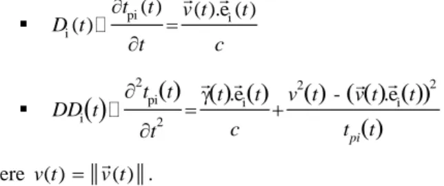
ij j τ ei -e t v t t t t c = .Let define the first and second-order Doppler coefficients related to Hi at time t, as follows
▪ pi i i ( ) ( ).e ( ) ( ) t t v t t D t t c = ▪
( )
( ) ( ) ( )
( )
(
( ) ( )
)
( )
2 2 2 pi i i i 2 .e - .e pi t t t t v t v t t DD t c t t t = + where v t( )= v t( ) .It is useful to distinguish between sensors time scale and source time scale, i.e. to introduce the different time scales between the emission and the receptions (see figure below). Ignoring the noises terms and the coefficients i in (1), we
have
( )
( )
(
( )
)
( )
( )
(
( )
)
i i i pi i i i i pi 0 H M t S t S t S t t t c S f t S t t = + = + = = +
(7) that means t + tpi(t) = ti + tpi(0). (8) t ti t = 0 tpi(0) t t+tpi(t) ti = 0 ti tk tk = 0 tk tpk(0) t+tpk(t) ik(0) ik(t) (Hk) (Hi)Fig. 1 - time scales for emission and receptions Thus, we consider three different time scales
- the absolute scale t : the one of the source, - the relative scales ti related to the receivers Hi.
received signal must be established at time tpi(t). We will note
( )
i( )
e( ) ( )
ri e e e pi e i e H M t t t t t t t f t c = + = + = .The general relation which links S, Si and Sj can be
formu-lated as follows
( )
e i(
i( )
e)
j( )
j( )
eS t =S f t =S f t . In fact, (7) and (8) implies
( )
(
1( )
)
i i i i S t =S f− t .
For ti close to tri , that means ti = tri + t where t 0, let’s note
( )
(
)
(
-1(
)
)
(
( )
)
i i ri i ri i
' θ
S t S t +t = S f t +t = S t , then, for i j,
S
i'oθ
-1i=
S
'joθ
-1j .Thus S'i can be deduced from S'j by
( )
(
)
( )
(
)
( )
' ' -1 '
i joθ oθj i joθji S t = S t = S t . first-order Taylor series expansion of tpi(te)
If we note
( )
i( )
e( ) ( )
ri e e e pi e i e H M t t t t t t t f t c = + = + = ,a first-order series expansion of tpi(te) leads to
(
)
( )
( )
( )
( )
i e i e e e e i e e ri e ri e d d d d.
H M t f t t t t D t t c t t t t + + + + +=
=
Then( )
(
( )
)
ri e i e e dt t = +1 D t dt . For ti = tri + t with t 0,( )
( )
-1 i i e i e 1 t f t t D t = + + .The signal received on Hi corresponds to the emitted signal
S(te), with a delay tri(te) and expanded or compressed
accord-ing to the value of Di(te).
With our hypotheses, the function ji can be calculated as
( )
( )
( )
j e ji i e 1 θ 1 D t t t D t + = + . (9)Usually, the speed of the source can be considered very small beside c, so Di(te) and Dj(te) are very small beside 1; we
can approximate ji(t) by the following expression
ji(t) (1+Dj(te)) (1-Dj(te)) t
or
ji(t) (1+Dj(te)-Dj(te)) t = (1+Dji(te)) t
where Dji(te) is the first-order differential Doppler coefficient
related to Hj and Hi. Then S'i can be deduced from S'j by the
linear relation
' '
(
(
( )
)
)
i( ) j 1 ji e S t =S +D t t
second-order Taylor series expansion of tpi(te)
If the acceleration of the target is no more negligible, a second-order series expansion of tpi(te) must be used, leading
to
(
)
( )
( )
( )
i e i e e e e 2 1 i e e 2 i e e ri ri d d ... ... d d d H M t f t t t t c D t t DD t t t t + = + + + + + = + or ri e i( )
e e 1 i( )
e e2 2 dt =dt +D t dt + DD t dt . In that case,( )
( )
( )
(
)
2 i 3 θ ( ) 1 2 1 i e e i e i e t DD t t t t D t D t + − + + .The calculation of ji(t) leads to
( )
( )
(
)
( )
( )
( )
( )
ji 2 2 1 1 θ ( )= ... 1 2 1 ( ) 1 ... 1 j e i e i e j e j e i e i e D t t t D t D t D t DD t DD t t D t + + + + + − +
(10)For the same reasons described above, Di(te), Dj(te), DDi(te), and DDj(te) are very small beside 1, and we can approximate ji(t) by the following expression
ji(t) (1+Dji(te)) t + DDji(te) t2,
where DDji(te) is the second-order differential Doppler coef-ficient related to Hj and Hi. We easily see that DDji(te) can be approximated by
( )
1(
( )
( )
)
2
ji e j e i e
DD t DD t −DD t .
In that case S'i can be deduced from S'j by a parabolic relation
( )
(
(
( )
)
( )
)
' ' 2
1
i j ji e ji e
S t =S +D t t+DD t t .
In both cases, the signals S'i and S'j correspond one to the
other except for the transformation ij(t).
The function ij(t) must be defined on a duration T’
corre-sponding to the integration time necessary for the evaluation of the function fij defined above. For a fixed value of T’, we
will be able to validate, according to the speed of the target, the first-order expansion of i(t) and j(t).
Extension of the ambiguity function
If Sj is the signal of reference, we can modify Si so that it
becomes comparable to Sj from the cross-correlative point of
view. For non-stationary signals, ij() defined by (5) is used
instead of the cross-correlation function. The transformation ij, previously presented, is used with coefficients noted D
and DD
ji(t) (1+D) t + DD t2 .
The estimated cross-correlation function ˆ (τ, ,ij D DD) can be written
(
)
(
)
' 2 '
i j j j j j
1 b (1 ) . τ d
b a a−
S +D t +DD t S t − t .This is the cross-ambiguity function [4] which depends on three parameters. As seen above, this expression can be sim-plified if the acceleration of the target is negligible (then DD=0). In fact, we could create a function with more pa-rameters, considering a higher order series expansion of tpi(te). Experiments show that the maximum of ˆ (τ, ,ij D DD)
is reached for ij, Dij and DDij which are respectively the
differential time delay, the first and second-order differential Doppler coefficients.
T = b-a is the integration time. The estimation of ij is
op-timal for the good parameters Dij and DDij, otherwise it is a
sub-optimal estimation. It has been proved [1] that the error of the estimation of ij is
ij ij
ij ij
ij 1 ˆ ˆτ -τ -1 2 b a D D D + = + E E .To have an unbiased estimation, it is necessary to choose
2
T
a=− and
2
T
b = . The variance of this estimator is [1]
(
)
(
)
(
)
2 2 2 ij ij ij ij 2 ij 1 ˆ ˆτ -τ -12 1+ D D DT
=
E E . resultsNow, we present some results of calculated envelopes of cross-correlation functions obtained with and without a cor-rection of the signal distortions. The figures above show the envelopes of the cross-correlation between receivers H11 and
H14 ; the first one with no correction (D=0 and DD=0) and
the second one with the optimal Doppler compensation (D=0.6% ; DD=0 because, in this case, the acceleration is negligible). 0 0.005 0.01 0.015 -30 -20 -10 0 10 20 30 Delay (ms)
Fig. 2. envelope of the correlation with no compensation
0 0.02 0.04 0.06 0.08 -30 -20 -10 0 10 20 30 delay (ms)
Fig. 3 - optimal cut of the ambiguity function
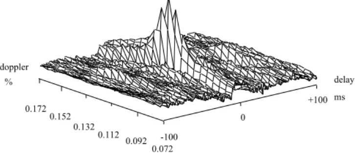
Without correction, no peak stands out. However, a peak emerges after a first-order Doppler compensation. The cross-ambiguity function between the signals received on hydro-phones H11 and H12 is shown below. Fifty first-order Doppler
coefficients were used with a 0.02% step, from 0.072% to 0.172%. In this case, the maximum is reached for ij = 33 ms
and Dij = 0.122 %. doppler % -100 +100 0 delay ms 0.172 0.152 0.132 0.112 0.092 0.072
Fig. 4 - ambiguity function between the signals received on H11 and H12
The problem of multiple reflections model and choice of a method
The presence of signal reflections on the sea bed can be modeled as follows ; the signal received on a sensor Hi is
i( ) ( pi) 1ik ( pi τ )ik i( )
R N k
S t =S t t− +
=r S t t− −+
B t (11) where NR is the number of reflected signals, ik is the delay ofthe k-th reflection and rik is the magnitude of each reflected
signal. The reflections modulate the spectral power density, destroy the coherence in certain frequency areas and create secondary peaks in the cross-correlation function, introducing errors on differential propagation delay estimation. General-ized cross-correlation methods, as SCOT, cannot eliminate secondary peaks due to reflections [6].
In theory, the finite MA model (11) can be approximated by an infinite AR model. Practically, a finite AR model must be used, and the order p must be chosen large enough to take into account the secondary peaks and make them disappear. This AR model is also used to whiten the received signals. It is indeed possible to interpret the emitted signal as the re-sponse of a linear filter to a white noise. By reversing the AR filter, we estimate the input white noise or innovation n and
then we realize the whitening of the signals [7][8]. This whit-ening is performed on raw data, and the correlation function is then calculated on transformed signals.
practical development
The choice of the AR order p is delicate, and several crite-ria have been proposed as SVD analysis of the covacrite-riance matrix [12]. To achieve the estimation of the model parame-ters, the Yule-Walker equations could be used. The estima-tion of this parameters can also be performed from raw data, commonly based on a least mean square-error of prediction of the signal criterion. Two classes of methods are possible, using the forward prediction or the forward and the backward predictions.
Lattice filters are commonly used to perform this calcula-tion [30]. We can define a basic seccalcula-tion linked to the
evolu-tion of the pth-order (forward and backward) predicevolu-tion er-rors ep(t) and rp(t) from the (p-1)th-order errors. It leads to a
system of recursive equations on both time and order
k k-1 k k-1 * k k-1 k k-1 1 1 ( ) ( ) ( ) ( ) ( ) ( ) e t e t K r t r t r t K e t − − = − = − (12)with two indices : k for order (k=0,…p) and t for time. Kk and *
k
K are the PARCOR (partial correlation) coefficients and are calculated to minimize a weighted least-squares criterion
(
2 2)
0 ( ) ( ) t t u k k u P − e t r t = =
+where is a forgetting factor verifying “ 1”. We find
k-1
k-1
* k k 2 2 k-1 k-1 ( ) ( 1) ( ) ( 1) 2 t t t t e r K K e r − − = = + E E E .(12) leads to the following basic lattice section ek-1(t) rk-1(t-1) ek(t) rk(t) -K*k -Kk
+
+
Fig. 5 - basic section (number k) of the lattice filter
Putting p basic lattice sections one after the other, a ‘pth-order inverse filter’ is realized (figure above).
e0(t) r0(t) z-1 x(t) (1) e1(t) r1(t) z-1 (2) ep-1(t) rp-1(t) z-1 (p) ep(t) rp(t)
Fig. 6 – pth-order AR model : lattice filter
If x(t) is the signal received on one sensor, en(t) is the
forward residual error which is white if the process is really a AR process. Hence applying this filter to the signals Si(t)
amounts to whitening them. The final basic schema is the following Si
AR
SjAR
ei ej ij ambiguityFig. 7 - basic scheme of the whitening procedure It is pivotal to apply the same transformation to the whole signals so that, even though the spectra are modified, this method does not modify the phase of the cross-spectrum, and the abscissa of the peak of the cross-correlation function is not shifted.
Furthermore, such a method can be slightly modified to process non-stationary data, and can be implemented to pro-cess data in real time; finally, normalized methods can im-prove precision and convergence speed of calculation.
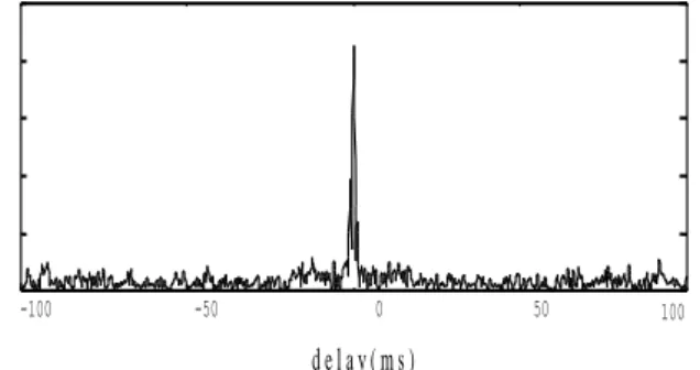
A convincing result is presented below ; the figures 8 and
9 show the cross-correlation obtained with the SCOT whiten-ing method : secondary peaks are clearly present on both sides of the main peak. The figure 10 shows the cross-correlation obtained with a AR model with an order p=100 : secondary peaks close to the main one have been seriously softened.
In fact, this method does not eliminate the secondary peaks, but push them away the main peak while reducing their magnitude. Thus, the order of the AR model must be chosen all the larger than the peaks are high or far away the main peak
delay (ms)
Fig. 8 - envelope of the cross-correlation function with sec-ondary peaks due to reflections on the sea bed (H11 - H14)
Fig. 9 - envelope of the cross-correlation function with sec-ondary peaks due to reflections on the sea bed (H11 - H12)
-100 -50 0 50 100
d e l a y ( m s )
Fig. 10 - envelope of the cross-correlation function with reduced reflections effects
4. Tracking
Introduction
We want to calculate one point of the trajectory every t second. From experiments, we will take t = 1 s for a surface vessel and less for a fast underwater target. The choice of t is linked to the possible dynamic evolutions of the target. It must be small enough to assure that the coordinates of the ambiguity function peak at time t+t are close to the values found at time t ; that means that the prospecting area of the parameters (, D and DD) is restricted to a priori defined values.
Practical method description : long baseline system
We suppose that at each time t we are able to estimate ij,
Dij and DDij as described before, for every available couple of
receivers. As seen before, to ensure that these parameters correspond to the same emission time, we must choose a sensor of reference H1 ; the others will be used to create pairs.
A Doppler compensation of S1 is required to make it
comparable to other received signals : that means a compres-sion or dilatation of this signal, obtained by an interpolation
t’ = (1+D) t + DD t2 ,
because we took a second-order Doppler compensation as a limit. All the transformations are performed at the same time on the signal of reference S1. The cross-ambiguity function is
computed at the same time between some receiving pairs ; M, v→ and → (state of the target) S1 S2 12 D12 DD12 processing S1 SN 1N D1N DD1N processing
We can evaluate the position M(te), the speed v t
( )
e and the acceleration γ( )
te of the target with the following system* τij
( )
te H M tj( )
e H M ti( )
e c −=
*( )
( )
( )
i e ij e j e 1 1 D t D t D t + = + *( )
( )
(
)
( )
( )
( )
( )
i e ij e 2 j e e j e i e i 1 1+ = -1+ 2 1+ D t DD t DD t DD t D t D t
by taking into account (3), (9) and (10). Then, the approxima-tion to the state of the target for te+t is
(
)
( )
( )
( )
(
) ( )
( )
(
) ( )
2 e e e e e e e e e 1 . 2 . M t t M t t v t t t v t t v t t t t t t + = + + + = + + =
As said above, it delimits the prospecting area of the parame-ters , D and DD at time t+t. This process can be repeated at time t+2t, and so on.
A trajectory obtained with real signals emitted by a sur-face vessel on the T.F.F. is shown on the following figure, where DD was assumed to be null, so (te) could not be reached
Fig. 11 - result of the target tracking
Theoretically at least 3 pairs are necessary to estimate the state of the target. With four pairs, it is possible to estimate the value of c instead of fixing its value a priori : of course the estimation is a constant value. Practically, proceeding that way, the estimation of the state of the target becomes better.
An extended Kalman filter can been used to estimate a priori position and speed at time t+t (and then differential time delay and Doppler coefficients), used to initialize algo-rithms even if previous calculations at times t, t-t, t-2t,… did not permit to estimate these parameters.
The estimation of the ambiguity function has been re-stricted to 3 parameters ; that means the Doppler compensa-tion has been restricted to the second-order. We could have used a third-order correction to improve results, especially for fast target. The cost for a better precision would be a higher sum of computation.
Estimation errors
The error on the position is difficult to reckon, because we do not know exactly where the supposed punctual source is located. It is probably situated at the back of the target (owing to the propellers, cavitation,…) as it will appear in the next study. It is difficult to compare the passive trajectory with a radar trajectory obtained with a reflector put on the middle of the target, because the tracking point is not the same in the both cases. The error between the trajectories is almost constant in the straight parts in comparison with the half size of the target. The tracking ‘point’ is located in the back of the target. In some cases, for active trajectory, we have noted a bad zero point because the radar was not satis-factorily calibrated.
Therefore we evaluate the errors on the position M(te)
cross-ambiguity function: ij and Dij. The available results
are the position, the speed and the associated errors.
Following, we can have a cartography of the maximum position error in the new Tremail range. Experiments have shown a maximum value of 0.5 ms for ij.
With this value, we can calculate, a cartography of the maximum error occurring in the future Tremail range.
Practical difficulties
Practically, two sorts of difficulties are encountered : physical difficulties
To ensure a precise decision, the signals from two receiv-ers must keep a minimal mutual coherence to make emerge a peak from the ambiguity function. As experiments have shown, this condition is not necessarily verified when the angle =
(
H M MHi , j)
tends to . Then, the Doppler influence is greater and a second-order Doppler compensa-tion may be insufficient. Then, the multiple refleccompensa-tions of different natures increase the dissymmetry between received signals. Finally, the dissymmetry of the radiation diagrams of the source is maximum in this configuration.Obviously, the signal to noise ratio is a determining factor for the quality of the tracking.
calculation difficulties
They mainly appear during the initialization phase, and are due to the large possible range of delays and Doppler coefficients, which grow with the angle and the distance between the receivers. The computation of the ambiguity function is so heavy that we cannot have access to a priori knowledge about the speed and the position of the target.
Conclusion
With the Tremail range in passive listening, we have shown that it is possible to obtain the trajectory of surface or underwater targets. In the multiple cases which are consid-ered, we have given the trajectory of the targets.
Because the possible ranges of parameters are very wide, the initialization procedure requires a lot of computations. The position of the hydrophones can be improved to allow passive tracking in a shorter time. It is necessary to create pairs of near receivers to improve results and to facilitate the initialization procedure. The distance chosen between the receivers of a pair will be about 100 m because noises on two receivers must remain uncorrelated and the respect of this condition imposes that the distance cannot be indefinitely decreased. In addition, an existing pair (H11-H12 distant of
100m) gave satisfying ambiguity functions.
This necessary short baseline system is described in the following section, and then mixed with the long baseline one to create a complete and autonomous system for tracking.
Of course, at least 3 pairs are necessary to perform a 3D tracking. But, as a precautionary measure, we will create more pairs.
5. Tracking mixing short and long baseline systems Introduction
As mentioned above, the previous method (long baseline system) has to be modified ; a reference pair of receivers, the first one (H11,H12), is chosen ; a pair of receivers is noted
(Hi1,Hi2) with i=1 to Np the number of pairs.
This section aims at developing the short baseline system and mixing it with the long baseline system.
The different ambiguity functions lead to differential time delays i linked to the pair (Hi1,Hi2). As Np pairs are available, we have Np equations (i=1 to Np)
Hi1M - Hi2M = c i . (13)
Principle of the evaluation of the target position
The position of the target M(te), is obtained by
conver-gence of a gradient method. We define the error associated to a pair
i = Hi1M - Hi2M - c i .
We want to minimize the following criterion J(M) = 1 2 i ε N i p =
.A recursive algorithm converges towards the real position of the target (corresponding to the delays i) is performed.
Experiments and simulations have shown that the conver-gence is ensured in the Tremail range.
Evaluation of the error on the position of the target
The new Tremail range is based on coupled sensors ; it tends to decrease the z component (depth) of gradients wi
where wi=gi1-gi2 and gij is the gradient of H Mij M M= '. The location precision on depth will be insufficient. So, it is nec-essary to study horizontal precision (x and y) for a fixed z.
Equations (13) represent hyperboloids. For a fixed z, the set of points that verify them are curves whose parameters are the i. For a delay k’ [k−k, k+k], we have a strip on
the z-plane. The intersection between two strips provides the area D where each point M' verifies
' i1 i2 i ' j1 j2 j ' ' .τ ' ' .τ H M H M c H M H M c − = − =
with k' [k−k, k+k] for k = {i,j}.
For simulations, imaginary hydrophones are created ; for example, if we consider two pairs H23-H231 and H24-H241 by
adding the imaginary hydrophones H231 and H241, the domain
D looks like on the figure below.
Four pairs are available for the short baseline system, de-signing an other domain D. For a finite number K of points {Mi} taken on the outline of D, we define a criterion to
quan-tify the maximal mean error on the position of the target for a fixed value of r i i=1 1 K MM K =
.Fig. 12 - precision on the position estimation of source for 2 pairs of sensors (H23-H231 and H24-H241)
The evaluation of the coordinates of Mi is performed with
the following system, where the position error is Mi = Mi - M
and wi is the gradient vector at point M.
p p 1 1 N N T k i k k k k k w w M w = = =
.The figure below represents the graph of the error r
ob-tained for a depth z = -100 m.
Fig. 13 - position error for z = -100 m
The error ranges between two meters in the center of Tremail and more than twenty meters on the sides.
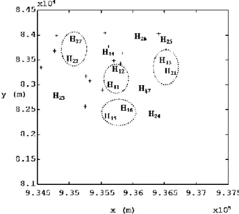
For the needs of our problem, using the existing pair H11
-H12, three new pairs are created : H22-H27, H15-H16 and H13
-H21. Four pairs are then available for the short baseline
sys-tem, designing an other domain D. We can see below the new T.F.F., proposed after the present study ; new receivers have been added to create near couples (H11-H12, H22-H27, H15-H16,
H13-H21).
The new Tremail owns near receivers; with these pairs, it is not possible to form coupling system with one sensor of reference as previously discussed. With this short baseline, it is necessary to adapt a new method associated to the four pairs.
Fig. 14 - new Tremail configuration
Initialization of a tracking
The Tremail range has been changed ; so, we have to define a new simple initialization mechanism with the short baseline system. This procedure can also be used when the target is lost. In this configuration, it is impossible to take a unique reference sensor to determine all the ambiguity func-tions. In this problem, the position, the speed and the acceler-ation of the target, and also the emission time te and then
reception times tri(te) are unknown. The wave emitted at time
te arrives on the receiver of reference of each pair at
( )
i1 e ri( )e e H M t t t t c = + .Fig. 15 - position of the target and pairs of sensors Because the position is indeterminate, the reception times for each pair is unknown. Assuming we calculate the ambigu-ity functions for the same reception time, the maximum error in the reception times is linked to the greatest distance be-tween the pairs of receivers : for T.F.F., it is about one sec-ond.
(
i1 j1)
max max p i, j 1; H H c T = Nwhere Hi1 is the first receiver of the i-th pair.
The calculation of ambiguity functions for the same re-ception time for all the pairs does not tally with a real
posi-tion of the target. But we can find a posiposi-tion that minimizes the mean square error, which cannot be a real position. Hav-ing found this estimate position, we can modify the reception time for each pair except for one that we do not change and that is considered like the reference pair.
Consider a pair of reference, called number one. Calcula-tion of propagaCalcula-tion delays for recepCalcula-tion times are initialized as follows for each pair
( )
(0) i riτ t with tri(0) =tr1(0) =i 1,...,Np.
The minimization of the mean square error allows us to estimate the position of the target M0 ; this permits to readjust
the reception time tri(1). The same reception time is kept for the reference pair. We have
11 0 i1 0 (1) (0) ri r1 H M H M t t c − = − .
A new evaluation of delays i at times tri(1), by ambiguity
functions, allows us to calculate M1.
A convergence by iterations towards the position of the source is performed. All experiments and simulations related to studied targets showed the convergence is reached. The criterion used to stop iterations is
N N (n) (n+1) (n) (n+1) ri ri ri ri i=1 i=2 t −t = t −t
.In a second stage, we can approximate the differential propagation delay i(tri(j+1)) by the first-order series expansion
in the neighborhood of tri(j)
( ) ( ) (
(j+1) (j) (j+1) (j)) ( )
i (j) i ri i ri ri ri ri τ τ t τ t t t t t = + − where τi( )
tri(j) t denotes the differential Doppler. This
ap-proximation is always justified with the chosen configura-tions.
We have to solve the following system of equations Hi1M - Hi2M = cτ ti
( )
ri , =i 1,...,Np. (14)Let suppose that each τ ti
( )
ri(0) is calculated by the ambigui-ty functions. A series expansion of (14) around tri(0) leads to( )
(0) (0) (0) i( )
(0) i1 i2 i r1 ri 1 r1 τ - τ ( - r ) H M H M c t c t t t t = + By definition(
(0) (0))
r1 ri 11 i1 c t−
t=
H M −H M , so that for all i, we obtain the following system( )
(
i (0))
i( )
(0)( )
(0) r1 i1 i2 11 r1 i r1 τ τ 1 - t H M H M H M t cτ t t t − + = which is solved by iterations by a mean square error minimi-zation.
Conclusion
A process has been proposed for position estimation in
the case of tracking initialization ; the speed of the target can also be estimated in the same way by a second-order series expansion of i(tri(j+1)) in the neighborhood of
(j) ri
t .
From differential time delays and Doppler coefficients computed for all pairs at reception time tr1(0), it is possible to evaluate the parameters of the target and the associated time.
This procedure is attractive because the distance between the two receivers of a pair is small and consequently the delays and Doppler ranges are reduced. This advantage is also a handicap for the precision on the estimated parameters. The result obtained by this short baseline system proce-dure is used to initialize the long baseline system proceproce-dure described in the previous section. With this second method, the results are obtained with an increased accuracy. As long as the target is efficiently tracked, this procedure is used. In the case where the target is lost while tracked with the long baseline procedure, the short baseline procedure is launched.
6. The tracking machine
Presentation
A passive tracking machine, based on the principle pre-sented before, containing a two channels numerical acquisi-tion board and several specific fast calculaacquisi-tion boards, has been built in order to perform real time evaluation of differ-ential time delay and first-order Doppler coefficient for one pair of receivers. An a posteriori trajectory calculation can also be performed because received signals are recorded on a magnetic tape.
Experimental results
The trajectory shown below (fig. 16) was obtained (one point every second), using four pairs of receivers, with sig-nals emitted by a fast patrol boat doing 15-20 knots during 3 minutes. About 15 minutes were needed to reconstruct. The part of the trajectory used contains a straight line and a curved part in order to better appreciate the quality of pro-cesses. The sampling frequency is 10 kHz (the useful fre-quency band is [100 Hz ;3 kHz]); integration time was taken equal to 1 s; 21 different Dopplers (first-order) were comput-ed for each point of trajectory. The trajectory obtaincomput-ed simul-taneously by a radar is superposed.
Absurd points are present on the passive trajectory (figure 17) ; in fact, this test underscored a problem due to the acqui-sition board of the tracking machine (a disturbing correlation between the two channels present for = 0).
The error made on the estimated position (by the passive method) is difficult to evaluate, because we do not know exactly where the supposed punctual source is located. How-ever, it seems more likely that it comes from the back of the target (owing to the propellers, cavitation, …).
Furthermore, it is difficult to compare the passive trajec-tory with the radar trajectrajec-tory obtained with a reflector put on the middle of the target, because the tracking point is not the same in the two cases. The error between both trajectories is almost constant in the straight line parts compared to the half size of the target. In some case, for active trajectory, we have noted a bad zero point because the radar is not satisfactorily calibrated.
(m)
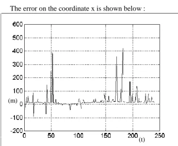
(m) Fig. 16 - passively estimated and radar trajectories The error on the coordinate x is shown below :
(t) (m)
Fig. 17 - x error between estimated and radar trajectories. Disregarding the absurd points (most of which could easi-ly be eliminated), a difference of about 15 metres can be seen, probably due to a too strong smoothing of the radar trajectory. After a suited correction of the acquisition board, the result obtained is the following (this is not the same part of the trajectory than above) .
The figure 18 shows the trajectory (projected on the hori-zontal plane x-y) obtained a posteriori for an underwater target during 15 seconds. A point is computed on every 0.5 s. The sampling frequency is 48 kHz (the useful frequency band is [100 Hz;20 kHz]); integration time is taken equal to 0.5 second; 49 different first-order Dopplers were used for each point of the trajectory during the initialization phase, 15 only during the tracking phase. No second-order Doppler compen-sation was made here. No radar could be used during this test. Much less absurd points are present (figure 19).
On the figure 20, each estimated point is drawn with a vector whose direction and length represent those of the esti-mated speed vector. The target goes from right to left. This figure is zoomed ; this is why the right part of trajectory is lacking.
In all cases, the trajectories obtained were satisfactory. Nevertheless, for such targets, a second-order Doppler
com-pensation becomes necessary to avoid the loss of the target, especially during turns.
(m)
(m)
Fig. 18 - passively estimated and radar trajectories
(m)
(t)
Fig. 19 - x error between estimated and radar trajectories
(m)
(m)
Fig. 20 - x-y cut of a 3D path of an underwater target
7. Conclusion
This study shows the feasibility of underwater passive tracking with the Tremail system. This feasibility is built from real signals that surface or underwater targets emit.