Approximation of the Integrals of the Gaussian Distribution of Asperity Heights in the Greenwood-Tripp Contact Model of Two Rough Surfaces Revisited

HAL Id: hal-01278038

https://hal.archives-ouvertes.fr/hal-01278038

Submitted on 3 Dec 2019

HAL is a multi-disciplinary open access

archive for the deposit and dissemination of

sci-entific research documents, whether they are

pub-lished or not. The documents may come from

teaching and research institutions in France or

abroad, or from public or private research centers.

L’archive ouverte pluridisciplinaire HAL, est

destinée au dépôt et à la diffusion de documents

scientifiques de niveau recherche, publiés ou non,

émanant des établissements d’enseignement et de

recherche français ou étrangers, des laboratoires

publics ou privés.

Distributed under a Creative Commons Attribution| 4.0 International License

Approximation of the Integrals of the Gaussian

Distribution of Asperity Heights in the

Greenwood-Tripp Contact Model of Two Rough Surfaces

Revisited

Radoslaw Jedynak, Jacek Gilewicz

To cite this version:

Radoslaw Jedynak, Jacek Gilewicz.

Approximation of the Integrals of the Gaussian

Distribu-tion of Asperity Heights in the Greenwood-Tripp Contact Model of Two Rough Surfaces

Revis-ited. Journal of Applied Mathematics, Hindawi Publishing Corporation, 2013, 2013, 459280 (7 p.).

�10.1155/2013/459280�. �hal-01278038�

Volume 2013, Article ID 459280,7pages

http://dx.doi.org/10.1155/2013/459280

Research Article

Approximation of the Integrals of the Gaussian Distribution of

Asperity Heights in the Greenwood-Tripp Contact Model of Two

Rough Surfaces Revisited

Rados

Baw Jedynak

and Jacek Gilewicz

1_{Kazimierz Pulaski University of Technology and Humanities, UL. Malczewskiego 20a, 26-600 Radom, Poland} 2_{Centre de Physique Th´eorique, CNRS, Luminy Case 907, Aix-Marseille Universit´e, UMR 6207,}

Universit´e Sud Toulon-Var, 13288 Marseille Cedex 09, France

Correspondence should be addressed to Radosław Jedynak; jedynakr@pr.radom.pl Received 6 February 2013; Revised 6 May 2013; Accepted 7 May 2013

Academic Editor: Renat Zhdanov

Copyright © 2013 R. Jedynak and J. Gilewicz. This is an open access article distributed under the Creative Commons Attribution License, which permits unrestricted use, distribution, and reproduction in any medium, provided the original work is properly cited.

Some examples of application of Pad´e approximant techniques to approximate the integrals in question and comparison with previ-ous results, essentially the recent Panayi-Schock and Green-wood results, show the efficiency of this simple natural approximation.

1. Introduction

Modelling of the contact between moving rough surfaces allows a better understanding of friction and wear mech-anisms, which can be used in engineering solutions. This issue has been examined using a number of approaches. The statistical type of a contact model is still the most popular model used in rough surfaces contact. This statement does not mean that it is the best solution of contact rough surfaces. Instead of using the complete roughness data, only probability density function is used. This function means the

probability of the asperity with the height between ℎ and

ℎ + 𝑑ℎ. The first well-known statistical model was introduced by Greenwood and Williamson [1] (GW). They joined a statistical process with a classical Hertzian contact to deal with the rough surfaces contact. They adopted the following

assumptions:(1) the asperity height distribution is Gaussian,

(2) asperity contact is modelled by the Hertzian spherical

contact theory,(3) the asperity tip radius is assumed constant,

and (4) adhesion contact between asperities is ignored.

A rough surface was described by three parameters: (1)

standard deviation of asperity height distribution,(2) average

asperity summit radius of curvature, and(3) areal asperity

density. This model has been widely accepted and developed by numerous researchers. The main reason of its popularity

is its simplicity and it’s predictions are in accordance with the carried out experiments. Some interesting review articles

in the frame of dry friction are written by Bhushan [2, 3],

Buczkowski and Kleiber [4], and Jedynak and Sulek [5]. The model proposed by Greenwood and Tripp [6] (GT) extended the GW model to contact between two rough surfaces. They showed that the contact between two rough surfaces can be modelled by a contact between an equivalent single rough surface and a flat one. The equivalent rough surface is characterized by an asperity curvature and the peak-height distribution of the equivalent surface. They used the simple formula for a standard deviation of the statistical distribution as the square root of the sum of squares of the standard deviations of asperity height distributions on the two surfaces. The GT model gained large popularity in the field of elastohydrodynamic analysis, and all the following papers refer to [6]. The most frequently cited equations given by the GT model are for the following asperity contact area:

𝐴_𝑒= 𝜋2(𝜉𝜅𝜎)2𝐴𝐹₂(𝜆) (1)

and load carried by the following asperities:

𝑊_𝑒 =8√2

2 Journal of Applied Mathematics

where 𝜉𝜅𝜎—roughness parameter, 𝐴—nominal contact

area,—Stribeck oil film parameter, first defined by Stribeck

[3, 6] as 𝜆 = ℎ/𝜎, 𝐸∗—effective elastic modulus, and

𝐹₂, 𝐹_5/2(𝜆)—statistical functions introduced to match the

assumed Gaussian distribution of asperities.

A parameter,𝜆 (ratio of film thickness to the composite

roughness of the contiguous surfaces), is used to ascertain any boundary contributions, which occur because of asperity interactions. It is a very important parameter for EHD analysis because interruptions in a coherent film may occur

when𝜆 < 3 [7].

At this point, it is worth noting that GT equations are only valid for surfaces which have a Gaussian distribution of asperities. A lot of real engineering surfaces do not meet these requirements. For example, a typical analysis of the compression ring of a piston against the cylinder bore is not correct if we use a Gaussian distribution. Spencer et al. [8] showed that the bore usually has a liner insert, which is crosshatch honed, making a plateau geometry. This geometry provides a smooth surface to allow for hydrodynamic film buildup between the piston rings and the cylinder liner surface. On the basis of these facts we can definitely say that the mentioned surfaces do not have a Gaussian distribution of asperities ringcylinder.

On the other hand, cam-tappet contact is a good example for using the mentioned distribution. Both surfaces are well known to follow Gaussian topography. This kind of conjunc-tion is the most loaded contact in the valve train mechanism. Jedynak and Sulek [5] showed that some kinds of galvanic coatings have also a Gaussian distribution of asperities.

Many surfaces do not follow at least a symmetric Gaus-sian-type distribution. Some researchers assume that the rubber-type material has a symmetric Gaussian-type distri-bution, but it is against the actually presented results, for example, Prokopovich et al. [9]. This paper clearly shows skew-symmetric Gaussian-type distribution for rubber seals. The mechanism of friction generation in the seal conjunction is complex, arising from adhesion of rubber in contact with the moving interface, viscous action of a thin film of fluid, and deformation of seal asperities. The authors developed a friction model based on the said mechanisms and then performed tests at both nano- and component level scales. Because the topography of the examined surfaces was nonsymmetric Gaussian, they used an alternative approach

for adhesive friction, which is described in [3,10]. They found

that adhesion is a dominant mechanism of friction.

The GT model is still being superseded by better models. Recently, Chong et al. [11] presented a friction model at fractal level, combining the effects of asperity adhesion, elastoplastic deformation, and a thin adsorbed boundary active molecular layer. This model forms the basis for the development of a generic multispecies lubricant-random roughness surface methodology. They stated that traditional boundary friction models do not apply to randomly distributed topology.

Statistical functions𝐹_𝑛(ℎ) which are used in extended GT

and GW models have the following form:

𝐹_𝑛(ℎ) = 1 √2𝜋∫ ∞ ℎ (𝑠 − ℎ) 𝑛_𝑒−𝑠2_/2 𝑑𝑠, 𝑛 = 1₂, 1,3₂, 2,5₂. (3)

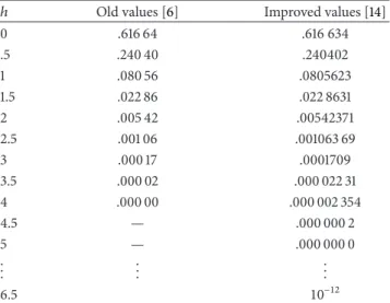
Table 1: Computed values of𝐹_5/2(ℎ) used to build the approxima-tion formulas.

ℎ Old values [6] Improved values [14]

0 .616 64 .616 634 .5 .240 40 .240402 1 .080 56 .0805623 1.5 .022 86 .022 8631 2 .005 42 .00542371 2.5 .001 06 .001063 69 3 .000 17 .0001709 3.5 .000 02 .000 022 31 4 .000 00 .000 002 354 4.5 — .000 000 2 5 — .000 000 0 .. . ... ... 6.5 10−12

This function can only be solved using numerical methods and that is why we discuss the most efficient approximations

formulas for𝐹_5/2(ℎ) in the next chapter. They are used by

many researchers in elastohydrodynamic analysis, In this case

𝐹_5/2is a function of𝜆. Then we propose a new formula which

is based on Pad´e approximation method.

It is important to emphasize that the approximations discussed next can be only applicable to surfaces which have a Gaussian distribution of asperities but not for all engineering surfaces which actually exist.

2. Previous Approximations

The GT model required the numerical integration of the Gaussian distribution. Greenwood and Tripp [6] provided tabulated results for this integral over its effective range: 9

points on the interval[0, 4], 0 ≤ 𝐹_𝑛 < 1 for all 𝑛, the last

digits given in [6] corresponded to10−5and fromℎ = 4 these

values were as follows:

𝐹_3/2(4) = 𝐹₂(4) = 𝐹_5/2(4) = 0.00000,

𝐹_𝑛(ℎ > 4) = 0. (4)

These values were recently used by a number of authors [7,

12,13] to approximate the integrals𝐹_𝑛 by simpler functions.

Unfortunately, all these authors used old tabulated values,

which were recently corrected [14] as shown inTable 1 for

𝐹_5/2(ℎ).

The following models of approximation of𝐹_5/2based on

the coefficient fitting to the tabulated values were proposed: (i) Hu et al. power law approximation [13]:

𝐹_5/2(𝐶)(ℎ) = 𝛼(4.0 − ℎ)𝛽 ℎ < 4.0,

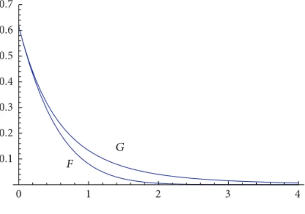
0 1 2 3 4 0.1 0.2 0.3 0.4 0.5 0.6 0.7 𝐺 𝐹

Figure 1: Graphs of𝐹_5/2(ℎ) and 𝐺_5/2(ℎ) for ℎ ∈ [0, 4].

(ii) Teodorescu et al. 5-degree polynomial approximation [7]:

𝐹_5/2(𝐴)(ℎ) = 𝑎0+ 𝑎1ℎ + ⋅ ⋅ ⋅ + 𝑎5ℎ5 ℎ < 4.0,

𝐹_5/2(ℎ ≥ 4) = 0, (6)

(iii) Panayi and Schock exponential form [12]:

𝐹_5/2(𝑃)(ℎ) = 𝑒(−.48347−1.65118ℎ+.06043ℎ2)/(1−.19256ℎ+.01610ℎ2)

− .00000350796 for ℎ < 4.0,

𝐹_5/2(𝑃)(ℎ ≥ 4) = 0,

(7)

(iv) Greenwood quartic fit to ln𝐹_𝑛[14]:

𝐹_5/2(𝐺)(ℎ) = .616634

× 𝑒.00121735ℎ4−.02342695ℎ3−.2696729ℎ2−1.7433954ℎ.

(8)

The paper [14] contains the analysis by Greenwood of the

paper [12], the corrected tabulated values of 𝐹_5/2, and the

model (7), which remains better than the Panayi-Schock model even after the correction of the coefficients in (6) by

the new values of𝐹_5/2. Greenwood proposed also in [14] to

consider the following modified function:

𝐺_𝑛(ℎ) = 𝑒ℎ2/2𝐹_𝑛(ℎ) (9)

which is more adapted to the numerical treatment, because it

is slower decreasing than𝐹_𝑛, as shown inFigure 1in the case

of𝑛 = 5/2.Figure 1shows both function𝐹_5/2(ℎ) and 𝐺_5/2(ℎ)

forℎ ∈ [0, 4].

3. Padé Approximation (PA) of

𝐹

or of

𝐺

The authors of the present paper are surprised that no Pad´e

approximation was tried to approximate𝐹_5/2 or𝐺_5/2 or to

approximate the integrated function. It is an automatic and low-cost method leading frequently to the surprisingly good results.

Let𝑓 be an analytic function at 𝑁 real different points

having the following power expansions: ∞

∑ 𝑘=0

𝑐_𝑘(𝑥_𝑗) (𝑥 − 𝑥_𝑗)𝑘, 𝑗 = 1, . . . , 𝑁. (10)

In practical situations, we know only a few first coefficients of each expansion, and then we have to deal with the limited information characterized by the following truncated power series: 𝑝𝑗−1 ∑ 𝑘=0 𝑐_𝑘(𝑥_𝑗) (𝑥 − 𝑥_𝑗)𝑘+ 𝑂 ((𝑥 − 𝑥_𝑗)𝑝_𝑗) , 𝑗 = 1, . . . , 𝑁. (11)

The𝑁-point Pad´e approximant (NPA) to 𝑓, if it exists, is a

rational function𝑃_𝑚/𝑄_𝑛 = [𝑚/𝑛] denoted, if it is needed, as

follows: [𝑚 𝑛] 𝑝1𝑝2⋅⋅⋅𝑝𝑁 𝑥1𝑥2⋅⋅⋅𝑥𝑁(𝑥) = 𝑎₀+ 𝑎₁𝑥 + ⋅ ⋅ ⋅ + 𝑎_𝑚𝑥𝑚 1 + 𝑏1𝑥 + ⋅ ⋅ ⋅ + 𝑏𝑛𝑥𝑛 , 𝑚 + 𝑛 + 1 = 𝑝 = 𝑝₁+ 𝑝₂+ ⋅ ⋅ ⋅ + 𝑝_𝑁 (12)

satisfying the following relations:

𝑓 (𝑥) − [𝑚_𝑛] (𝑥) = 𝑂 ((𝑥 − 𝑥𝑗)𝑝𝑗) , 𝑗 = 1, 2, . . . 𝑁. (13)

Each𝑝_𝑗represents the number of coefficients𝑐_𝑘(𝑥_𝑗) of

exp-ansion actually used for the computation of NPA. In the

present problem, all 𝑝_𝑗 = 1, and the construction of

NPA[𝑚/𝑛] is equivalent to the construction of the rational

interpolation 𝑃_𝑚/𝑄_𝑛. The classical Pad´e approximant (PA)

is a one-point PA computed from the development of the

function𝑓 at the origin 𝑥 = 0. It is defined by the linear

system obtained by the definition (13) with right-hand side

𝑂(𝑥𝑚+𝑛+1_).

At the first time, let us estimate crudely the function𝐹_5/2

by an exponential function in the interval[0, 4]:

𝐹_5/2(ℎ) = 𝛼𝑒−𝛽ℎ; 𝛼 = .616634; 𝛽 = −1 4ln .000002354 .616634 . (14)

Of course this simple interpolation over two nodes badly

reproduces𝐹_5/2on this interval; however, it shows that our

Pad´e approximant must decrease on [0, 4] (8) and must

become rapidly zero after. That is, the degree of its denom-inator must be sensibly greater than those of numerator.

To obtain the optimal results using the Pad´e

approxima-tion method, one must select the “best” PA[𝑚/𝑛]; it means

the “best” degrees 𝑚 and 𝑛. Many practical algorithms of

choice of the best PA were proposed in [15]. For the present

problem, we select two following algorithms: 𝜌-method

and the method of valleys in 𝑐-table, both based on the

analysis of the coefficients of the expansion of the considered

4 Journal of Applied Mathematics Table 2 𝑚 𝑛 0 1 2 3 4 5 6 7 8 0 1 .61 .38 .23 .145 .89-1 .55-1 .34-1 .21-1 1 1 −1.08 .49 −.12 .15-1 −.47-3 −.72-4 .104-5 .98-6 2 1 1.08 .30 .29-1 .11-2 .14-4 .10-6 .2-8 3 1 −.81 .12 −.45-2 .53-4 −.19-6 .16-9 4 1 .49 .33-1 .48-3 .18-5 .2-8 5 1 −.26 .75-2 −.38-4 .42-7 6 1 .12 .14-2 .24-5 7 1 −.053 .22-3 8 1 .021

{𝜌_𝑛 = |𝑐_𝑛/𝑐_𝑛+1|}. The nonmonotonicity of the few first terms

of{𝜌_𝑛}, if the presumed PA is such that 𝑚 > 𝑛, indicates the

difference𝑚 − 𝑛. The 𝑐-table is the table of determinants of

matrices of linear systems defining the denominators of the

classical (one-point) PA[𝑚/𝑛]: 𝐶𝑚_𝑛 = 󵄨󵄨󵄨󵄨 󵄨󵄨󵄨󵄨 󵄨󵄨󵄨󵄨 󵄨󵄨󵄨󵄨 󵄨󵄨 𝑐_𝑚 𝑐_𝑚−1 ⋅ ⋅ ⋅ 𝑐_{𝑚−𝑛+1} 𝑐_𝑚+1 𝑐_𝑚 ⋅ ⋅ ⋅ ⋅ ⋅ ⋅ .. . ... ... ... 𝑐𝑚+𝑛−1 ⋅ ⋅ ⋅ ⋅ ⋅ ⋅ 𝑐𝑚 󵄨󵄨󵄨󵄨 󵄨󵄨󵄨󵄨 󵄨󵄨󵄨󵄨 󵄨󵄨󵄨󵄨 󵄨󵄨 . (15)

At the same time, the dominant error of{𝑓 − [𝑚/𝑛]} near the

origin is proportional to𝐶𝑚_𝑛. The minima of each antidiagonal

in the table of |𝐶𝑚_𝑛|, of the entries builded with the same

information, indicate the paradiagonal with fixed𝑚 − 𝑛 of

the best PA.

By the integration of parts of (3), one obtains the following recurrence formulae:

𝐹_𝑛+1(ℎ) = 𝑛𝐹_𝑛−1(ℎ) − ℎ𝐹_𝑛(ℎ) . (16)

The following formulas for the derivatives are also useful to

obtain the development in power series of𝐹_𝑛:

𝐹_𝑛󸀠(ℎ) = −ℎ𝐹_𝑛(ℎ) − 𝐹_𝑛+1(ℎ) = −𝑛𝐹_𝑛−1(ℎ) . (17)

Now we can compute the expansion in the power series of

𝐹_5/2near the origin, where𝑎 := 𝐹_1/2(0) = .411089 and 𝑏 :=

𝐹_3/2(0) = .43002: 𝐹_5/2(ℎ) = (3𝑎₂ ) − (5𝑏₂) ℎ + (15𝑎₈ ) ℎ2− (5𝑏₈) ℎ3 + (5𝑎 64) ℎ4+ ( 𝑏 64) ℎ5− ( 𝑎 256) ℎ6 − ( 5𝑏 5376) ℎ7+ ⋅ ⋅ ⋅ = .616634 − 1.07505ℎ + .770793ℎ2− .268762ℎ3 + .0321164ℎ4+ .00671906ℎ5 − .00160582ℎ6− .000399944ℎ7 + .000100364ℎ8+ .0000249965ℎ9+ ⋅ ⋅ ⋅ , (18)

and the power series expansion of the function𝐺_5/2:

𝐺_5/2(ℎ) = 𝑒ℎ2/2𝐹_5/2(ℎ) = .61663422

− 1.07505ℎ + 1.07911ℎ2− .8062875ℎ3

+ .49459203ℎ4− .262043ℎ5+ .12364801ℎ6

− .0530326ℎ7+ .0209760ℎ8− .0077339ℎ9+ ⋅ ⋅ ⋅ .

(19)

The𝜌-method consists of the analysis of the regularity of the

sequence{𝜌_𝑛= |𝑐_𝑛/𝑐_𝑛+1|}. The beginning of the sequence {𝜌_𝑛}

corresponding to (19) is regular:

𝜌₀, 𝜌₁. . . 𝜌₇= .57, .996, 1.34, 1.63, 1.89, 2.12, 2.33, 2.53.

(20)

This indicates that the rational approximation{𝑚/𝑛}

corre-sponding to this series is such that𝑚 ≤ 𝑛. More significant

result is observed studying the𝑐-table corresponding to (19),

where the notation.1 − 5 means 0.1 × 10−5(seeTable 2).

The minima are located on the positions0/3, 1/4, 2/5 and

3/6. The best PA is then as follows:

[3₆] 𝐺(ℎ) = (.616634 + .0587436ℎ +.0186433ℎ2− .0000525721ℎ3) × (1. + 1.83868ℎ + 1.48582ℎ2+ .680187ℎ3 +.187771ℎ4+ .0300186ℎ5+ .0022127ℎ6)−1. (21)

InTable 3we compare the exact values of𝐹_5/2(ℎ) with those

obtained by multiplying [3/5]_𝐺 and [3/6]_𝐺 by 𝑒−(ℎ2/2) and

with the values calculated by the Greenwood approximation [14] and the Panayi approximation [12].

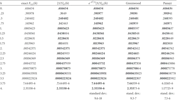
Clearly the [3/6] PA leads to the best values, but it is

computed with 10 coefficients (information) on𝐺_5/2atℎ = 0.

The results obtained with[3/5] PA (9 information) are better

in the range0÷2.5 than the Greenwood results (obtained also

Table 3: Approximation of𝐹_5/2via one point (ℎ = 0) Pad´e approximants of 𝐺_5/2.

ℎ exact𝐹_5/2(ℎ) 𝑒−ℎ2/2[3/5]_𝐺(ℎ) 𝑒−ℎ2/2[3/6]_𝐺(ℎ) Greenwood Panayi

0. .616634 .616634 .616634 .616634 .616636 .5 .240402 .240402 .240402 .240401 .240395 1. .0805623 .0805623 .0805623 .0805597 .0805637 1.5 .0228631 .0228627 .022863 .0228629 .0228449 2. .00542371 .00542304 .00542366 .00542412 .00541762 2.5 .00106369 .00106315 .00106365 .00106379 .00106965 3. .000170873 .000170616 .000170852 .000170864 .000175778 3.5 .0000223124 .0000222326 .0000223059 .000022307 .0000225912 4. 2.35338-6 2.33623-6 2.35197-6 2.35373-6 1.17725-9

The bold digits are exact.

Table 4: 9-point Pad´e approximation of𝐹_5/2obtained directly and also via approximation of𝐺_5/2. Comparison with Greenwood and Panayi results.

ℎ exact𝐹_5/2(ℎ) [3/5]_𝐹(ℎ) 𝑒−ℎ2/2[3/5]_𝐺(ℎ) Greenwood Panayi

0. .616634 .616634 .616634 .616634 .616636 .25 .391978 .3849 .391977 .39198 .391941 .5 .240402 .240402 .240402 .240401 .240395 .75 .141962 .142463 .141962 .141959 .141971 1. .0805623 .0805623 .0805623 .0805597 .0805637 1.25 .0438561 .0438004 .0438561 .0438548 .0438441 1.5 .0228631 .0228631 .0228631 .0228629 .0228449 1.75 .0113963 .0114051 .0113963 .0113967 .0113818 2. .00542371 .00542371 .00542371 .00542412 .00541762 2.25 .00246124 .00245933 .00246124 .0024615 .00246296 2.5 .00106369 .00106369 .00106369 .00106379 .00106965 2.75 .00043732 .000437939 .00043732 .000437338 .000443886 3. .000170873 .000170873 .000170873 .000170864 .000175778 3.25 .0000633931 .0000630551 .0000633931 .0000633825 .0000658778 3.5 .0000223124 .0000223124 .0000223124 .000022307 .0000225912 3.75 7.44495-6 .7.44495-6 7.44495-6 7.44359-6 6.11165-6 4. 2.35338-6 2.35338-6 2.35338-6 2.35373-6 1.17725-9

standard dev.: stand. dev.: stand. dev.:

9.6-18 9.3-7 7.3-6

The bold digits are exact.

from the development of a function near the origin gives good results in the neighborhood of the origin. In the following,

we will compare the𝑁-point PA [3/5]1 1⋅⋅⋅1_ℎ

1ℎ2⋅⋅⋅ℎ9and[3/6]

2 1⋅⋅⋅1

ℎ1ℎ2⋅⋅⋅ℎ9

with other results. The NPA[3/6], corresponding to our best

choice, is easily calculated with 9 values of 𝐺_5/2 and one

additional coefficient of development (19):

[3₅] 𝐺(ℎ) = (.616634 + .10073ℎ +.00818188ℎ2− .000161362ℎ3) × (1. + 1.90693ℎ + 1.58667ℎ2+ .740254ℎ3 +.19751ℎ4+ .0298511ℎ5)−1. (22)

Table 4contains the values of the approximations also in the

points located between the nodes, because the NPA are, of course, exact in the nodes, and we must analyze other points to compare our approximations with those of Greenwood and

Panayi. The advantage to determine the values of𝐹_5/2(ℎ) via

6 Journal of Applied Mathematics 1 2 3 4 4 × 10−6 2 × 10−6 −2 × 10−6 −4 × 10−6

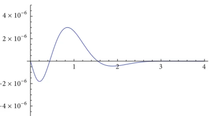
Figure 2: Graph of the error of Greenwood (7) approximation: 𝐹5/2(ℎ) − 𝐹5/2(𝐺)(ℎ). 1 2 3 4 4 × 10−6 2 × 10−6 −2 × 10−6 −4 × 10−6

Figure 3: Graph of the error of our approximation: 𝐹_5/2(ℎ) − 𝑒−(ℎ2/2)_[3/5]

𝐺(ℎ).

the intermediate points all digits exact and it is not the case

of the values of the NPA[3/5]_𝐹(ℎ) determined directly by the

values given in [14] (Table 1):

[3 5]𝐹(ℎ) = (.616634 − .457287ℎ +.1141502ℎ2− .0095798ℎ3) × (1. + 1.3788066ℎ − .997978ℎ2+ 2.988216ℎ3 −1.651924ℎ4+ .5588187ℎ5)−1. (23)

Figures2and3illustrate this fact clearly.

Here, we see that the simple NPA [3/5], that is, an

NPA builded with the same information that Greenwood or Panayi approximations, is the best. The comparison of the standard deviations is significant. Other advantage consists in its simple calculation. The following figures representing the error of our approximations illustrate the sharpness of our results.

It is possible to try other approximations using the Pad´e

techniques. One can use other interpolation nodes forℎ >

4 with values 𝐹_5/2(ℎ) = 0 and in particular the point

at infinity 𝐹_5/2(∞) = 0. For instance, if we compute 11

points Pad´e approximant[𝑚/𝑛] (𝑚 + 𝑛 + 1 = 11), we can

choose[0/10], [1/9], [2/8], [3/7], [4/6], . . . where the

behav-ior at infinity is, respectively:

𝛼₁ ℎ10, 𝛼₂ ℎ8, 𝛼₃ ℎ6, 𝛼₄ ℎ4, 𝛼₅ ℎ2, . . . , (24)

where𝛼_𝑖can be crudely estimated atℎ = 4 as follows:

𝛼₁= .000002354 × 410= 2.36; . . . ; 𝛼₅= .000002354 × 42.

(25) The numerical tests show that simple use of these additional nodes does not improve the approximation. The effect of appearing oscillations is negative.

The Pad´e approximant method allows, if it is needed, to obtain the two-sided estimates of the approximated function.

This consists of construction of one NPA[𝑚/𝑛] from 𝐾 =

𝑚+𝑛+1 given coefficients and of the second one, [𝑚−1/𝑛] or [𝑚/𝑛 − 1], with 𝐾 − 1 coefficients. In this case, if the first NPA is greater than approximated function between two nodes, the second is less than this function. Both NPA bound the approximated function from top and from below [16].

4. Conclusion

The efficiency of one-point as well as𝑁-point Pad´e

approx-imation method applied to the special tribology problem is presented and compared with other methods. This method starts from the choice of the best Pad´e approximant and is easily feasible. Our results confirm an ingenious idea of Greenwood proposing to approximate a modified function

𝐺_𝑛, more smooth that the function 𝐹_𝑛 (see Figure 1), and

then return to the calculus of 𝐹_𝑛, which allows to reduce

considerably the numerical errors.

Acknowledgment

The authors wish to thank the reviewers for their very con-structive and helpful comments which are important to improve the paper.

References

[1] J. A. Greenwood and J. B. P. Williamson, “Contact of nominally at surfaces,” Proceedings of the Royal Society A, vol. 295, pp. 300– 319, 1966.

[2] B. Bhushan, “Contact mechanics of rough surfaces in tribology: multiple asperity contact,” Tribology Letters, vol. 4, no. 1, pp. 1– 35, 1998.

[3] B. Bhushan, Handbook of Micro/Nanotechnology, CRC Press, 1999.

[4] R. Buczkowski and M. Kleiber, “Statistical models of rough surfaces for finite element 3D-contact analysis,” Archives of

Computational Methods in Engineering, vol. 16, no. 4, pp. 399–

424, 2009.

[5] R. Jedynak and M. Sulek, “Numerical and experimental inves-tigation of plastic interaction between rough surfaces,” Arabian

Journal for Science and Engineering. In press.

[6] J. A. Greenwood and J. H. Tripp, “The contact of two nominally at rough surfaces,” Proceedings of the Institution of Mechanical

[7] M. Teodorescu, M. Kushwaha, H. Rahnejat, and S. J. Rothberg, “Multi-physics analysis of valve train systems: from system level to microscale interactions,” Journal of Multi-Body Dynamics, vol. 221, no. 3, pp. 349–361, 2007.

[8] A. Spencer, A. Almqvist, and R. Larsson, “A numerical model to investigate the effect of honing angle on the hydrodynamic lubrication between a combustion engine piston ring and cylinder liner,” Journal of Engineering Tribology, vol. 225, no. 7, pp. 683–689, 2011.

[9] P. Prokopovich, S. Theodossiades, H. Rahnejat, and D. Hodson, “Friction in ultra-thin conjunction of valve seals of pressurised metered dose inhalers,” Wear, vol. 268, no. 5-6, pp. 845–852, 2010.

[10] R. Gohar and H. Rahnejat, Fundamentals of Tribology, Imperial College Press, 2008.

[11] W. W. F. Chong, M. Teodorescu, and H. Rahnejat, “Nanoscale elastoplastic ad-hesion of wet asperities,” Journal of Engineering

Tribology, 2013.

[12] A. P. Panayi and H. J. Schock, “Approximation of the integral of the asperity height distribution for the Greenwood-Tripp asperity contact model,” Journal of Engineering Tribology, vol. 222, no. 2, pp. 165–169, 2008.

[13] Y. Hu, H. S. Cheng, T. Arai, Y. Kobayashi, and S. Aoyama, “Numerical simulation of piston ring in mixed lubrication—a nonaxisymmetrical analysis,” Journal of Tribology, vol. 116, no. 3, pp. 470–478, 1994.

[14] J. A. Greenwood, “Approximation of the integral of the asperity height distribution for the Greenwood-Tripp asperity contact model,” Journal of Engineering Tribology, vol. 222, no. 7, pp. 995– 996, 2008.

[15] J. Gilewicz, Approximants de Pad´e, vol. 667 of Lecture Notes in

Mathematics, Springer, Berlin, Germany, 1978.

[16] R. Jedynak and J. Gilewicz:, “Approximation of smooth func-tions by weighted means of N-point Pade approximants,”

Submit your manuscripts at

http://www.hindawi.com

Hindawi Publishing Corporation

http://www.hindawi.com Volume 2014

Mathematics

Hindawi Publishing Corporation

http://www.hindawi.com Volume 2014

Mathematical Problems in Engineering

Hindawi Publishing Corporation http://www.hindawi.com

Differential Equations

International Journal of

Volume 2014

Applied MathematicsJournal of

Hindawi Publishing Corporation

http://www.hindawi.com Volume 2014

Probability and Statistics

Hindawi Publishing Corporation

http://www.hindawi.com Volume 2014

Journal of

Hindawi Publishing Corporation

http://www.hindawi.com Volume 2014 Mathematical PhysicsAdvances in

Complex Analysis

Hindawi Publishing Corporation

http://www.hindawi.com Volume 2014

Optimization

Hindawi Publishing Corporation

http://www.hindawi.com Volume 2014

Combinatorics

Hindawi Publishing Corporation

http://www.hindawi.com Volume 2014

International Journal of

Hindawi Publishing Corporation

http://www.hindawi.com Volume 2014

Operations ResearchAdvances in

Journal of

Hindawi Publishing Corporation

http://www.hindawi.com Volume 2014

Function Spaces

Abstract and Applied Analysis

Hindawi Publishing Corporation

http://www.hindawi.com Volume 2014 International Journal of Mathematics and Mathematical Sciences

Hindawi Publishing Corporation http://www.hindawi.com Volume 2014

The Scientific

World Journal

Hindawi Publishing Corporation

http://www.hindawi.com Volume 2014

Hindawi Publishing Corporation

http://www.hindawi.com Volume 2014

Algebra

Discrete Dynamics in Nature and Society Hindawi Publishing Corporation

http://www.hindawi.com Volume 2014 Hindawi Publishing Corporation

http://www.hindawi.com Volume 2014

Decision Sciences

Discrete Mathematics

Hindawi Publishing Corporation

http://www.hindawi.com Volume 2014 Hindawi Publishing Corporationhttp://www.hindawi.com Volume 2014

Stochastic Analysis