HAL Id: hal-02265778
https://hal.archives-ouvertes.fr/hal-02265778
Submitted on 12 Aug 2019HAL is a multi-disciplinary open access
archive for the deposit and dissemination of sci-entific research documents, whether they are pub-lished or not. The documents may come from
L’archive ouverte pluridisciplinaire HAL, est destinée au dépôt et à la diffusion de documents scientifiques de niveau recherche, publiés ou non, émanant des établissements d’enseignement et de
On the flavor structure of the light-quark sea
distributions
Jacques Soffer, Claude Bourrely
To cite this version:
Jacques Soffer, Claude Bourrely. On the flavor structure of the light-quark sea distributions. Nuclear Physics A, Elsevier, 2019, 991, pp.121607. �10.1016/j.nuclphysa.2019.08.001�. �hal-02265778�
On the flavor structure of the light-quark sea
distributions
Jacques Soffer
1,2 (deceased) andClaude Bourrely
11 Aix Marseille Univ, Universit´e de Toulon, CNRS, CPT, Marseille, France 2Physics Department, Temple University, 1925 N, 12th Street, Philadelphia,
PA 19122-1801, USA
Abstract
The flavor structure of the nucleon sea provides unique information to test the statistical parton distributions approach, which imposes strong relations between quark and antiquarks. These properties for unpolarized and helicity distributions have been verified up to now by recent data. We will emphasize the properties of the light-quark sea and present here some new results which are a real challenge for forthcoming accurate experimental results, mainly in the high Bjorken-x region.
Keywords: Statistical parton model, helicity parton distributions, sea quarks
0
1
Introduction
The structure of the nucleon sea is an important topic which has been the subject of several relevant review papers [1, 2]. In spite of considerable progress made in our understanding, several aspects remain to be clarified, which is the goal of this paper. The properties of the light quarks u and d, which are the main constituents of the nucleon, will be revisited in the quantum statistical parton distributions approach proposed more than one decade ago. These properties worth a separate presentation not developped in the original paper [3]. It is well known that the u quark dominates over the d quark, but for antiquarks, SU(2) symmetry was assumed for a long time, namely the equality for the corresponding antiquarks, ¯u = ¯d, leading to the Gottfried sum rule [4]. However, the NMC Collaboration [5] found that this sum rule is violated, giving a strong indication that ¯d > ¯u.
In the statistical approach we impose relations between quarks and an-tiquarks and we treat simultaneously unpolarized distributions and helicity distributions, which strongly constrain the parameters, a unique situation in the literature. As we will see, this powerful tool allows us to understand, not only the flavor symmetry breaking of the light sea, but also the Bjorken-x be-havior of all these distributions and to make challenging specific predictions for forthcoming experimental results, in particular, in the high-x region. The paper is organized as follow: in section 2 the main properties of the parton structure in the statistical model are explained. In section 3, we present a comparison of the results obtained by the model with unpolarized and po-larized experimental data, in the case of configuration associated with light sea quarks. Our conclusions are presented in section 4.
2
Structure of the parton statistical model
In our model the building blocks of the parton structure are the helicity components defined by the sum of two terms: a generic quasi Fermi-Dirac function
AqYqhxbq exp[(x − Yh
q )/¯x] + 1
where Yh
q are the thermodynamical potentials, ¯x plays the role of a universal temperature. The other term is a helicity independent diffractive contribution
˜ Aqx˜bq
exp(x/¯x) + 1, (2)
which controls the low x behavior of the distributions. This term is absent in the quark helicity distribution ∆q = q+− q−
, in the quark valence contri-bution q − ¯q and in u − d if one assumes ˜Au = ˜Ad.
A fit of unpolarized and polarized data leads to the solution given in Ref. [3] for the Parton Distribution Functions PDFs starting at the input energy scale Q2
0 = 1GeV2. For the quarks the helicity distributiions read:
xqh(x, Q2 0) = AqXqhxbq exp[(x − Xh q)/¯x] + 1 + A˜qx ˜bq exp(x/¯x) + 1 , (3) and for the antiquarks
x¯qh(x, Q20) = ¯ Aq(X −h q ) −1 x¯bq exp[(x + X−h q )/¯x] + 1 + A˜qx ˜bq exp(x/¯x) + 1 . (4) X±
q are the two thermodynamical potentials of the quark q, with helicity h = ±, the temperature has the value ¯x = 0.09. These potentials represent the fundamental parameters of the approach whose values are
Xu+ = 0.475±0.001, X − u = X
−
d = 0.307±0.001, Xd+ = 0.244±0.001. (5) The others parameters have the values:
Aq = 1.943 ± 0.005, bq = 0.471 ± 0.001 ¯Aq = 8.915 ± 0.050,
¯bq = 1.301 ± 0.004, ˜Aq = 0.147 ± 0.003, ˜bq = 0.0431 ± 0.003 . (6) The number of free parameters is reduced to seven by the valence sum rule,
R
(q(x) − ¯q(x))dx = Nq, where Nq = 2, 1 for u, d, respectively. In Eqs. (3,4) the multiplicative factors Xh
q and (X −h q )
−1
in the numerators of the first terms of the q’s and ¯q’s distributions, was justified in our attempt to generate the transverse momentum dependence of the PDFs [6].
Notice that following the chiral properties of QCD, we have Xh
q = −X −h ¯ q in the exponentials. In other parton models, unpolarized and polarized dis-tributions for quarks, antiquarks, are treated as four separated quantities,
while in the statistical model the appearance of the same potentials in q and ¯
q shows a strong relation between quarks and antiquarks. Looking at Eqs. (5) it turns out that two potentials X−
u, X −
d have iden-tical numerical values, so for light quarks results the following hierarchy between the different potential components
Xu+ > X − u = X
−
d > Xd+. (7)
We also notice that quark helicity PDFs increase with the potentials value, while antiquarks helicity PDFs increase when the potentials decrease.
The above hierarchy implies the following hierarchy on the quark helicity distributions for any x, Q2,
xu+(x, Q2) > xu−(x, Q2) = xd−(x, Q2) > xd+(x, Q2) , (8) and also the obvious hierarchy for the antiquarks, namely
x ¯d−(x, Q2) > x ¯d+(x, Q2) = x¯u+(x, Q2) > x¯u−(x, Q2). (9)
3
Light sea quarks results compared with
experiments
In several experiments an attempt is worked out to extract PDFs at a given x and Q2 values, which is a difficult task but useful to check the models. In this section a comparison between the predictions of our model and the available experimental data will be discussed, with an emphasize on the antiquarks contribution.
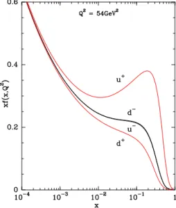
As a preliminary description of the helicity distributions structure we show in Figs. 1-2, the resulting distributions at Q2 = 54GeV2. This peculiar Q2 correspond to a measurement made by the E866 experiment [7, 8].
One sees in Fig. 1 that the largest distribution is indeed xu+(x, Q2), it has a distinct maximum around x = 0.3, which is also responsible for the maximum observed in the polarized structure function g1p(x, Q2) at the same x value.
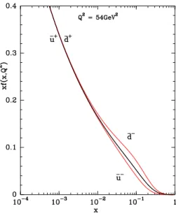
In Fig. 2, at large x, the distribution ¯d−
is slightly larger than ¯u− , this property implies that the ratio ¯d/¯u is larger than 1 and increasing with x, we will come back later to this point.
We have also checked that the initial analytic form Eqs. (3,4), is almost preserved by the Q2 evolution with some small changes of the parameters value.
This general pattern displayed in Figs. 1-2, does not change much for different Q2 values. In our approach one can conclude that, u(x, Q2) > d(x, Q2) implies a flavor symmetry breaking of the light sea, i.e. ¯d(x, Q2) > ¯
u(x, Q2), which is clearly seen in Fig. 2.
A simple interpretation of this result is a consequence of the Pauli exclu-sion principle, based on the fact that the proton contains two u quarks and only one d quark. It is important to note that these inequalities Eqs. (8,9) are preserved by the next-to-leading order QCD evolution, at least outside the diffractive region, namely for x > 0.1.
Figure 1: The different helicity components of the light quark distributions xf (x, Q2) (f = u
+, u−= d−, d+), versus x, at Q2 = 54GeV2, after NLO QCD evolution, from the initial scale Q2
0 = 1GeV2.
We now turn to more significant outcomes concerning the helicity distri-butions which follow from Eqs. (8,9). First for the u-quark
x∆u(x, Q2) > 0 x∆¯u(x, Q2) > 0. (10) Similarly for the d-quark
Figure 2: The different helicity components of the light antiquark distribu-tions xf (x, Q2) (f = ¯d
−, ¯d+ = ¯u+, ¯u−), versus x, at Q2 = 54GeV2, after NLO QCD evolution, from the initial scale Q2
0 = 1GeV2.
So once more, quarks and antiquarks are strongly related since opposite signs for the quark helicity distributions, imply opposite signs for the antiquark helicity distributions, (see Eqs. (3,4)), at variance with the simplifying flavor symmetry assumption x∆¯u(x, Q2) = x∆ ¯d(x, Q2).
Our predicted signs and magnitudes for distributions [3] have been con-firmed by the measured single-helicity asymmetry AL in the W
±
production at BNL-RHIC from STAR [9]. For the extraction of helicity distributions, this process is expected to be cleaner than semi-inclusive DIS, because it does not involve fragmentation functions.
Another important earlier prediction concerns the Deep Inelastic Scatter-ing (DIS) asymmetries, more precisely (∆q(x, Q2) + ∆¯q(x, Q2))/(q(x, Q2) +
¯
q(x, Q2)) (q = u, d), shown in Fig. 3. Note that the JLab [10] data and the COMPASS [11] data are in agreement with these predictions, in particular, in the high-x region where there is a great accuracy. Beyond x = 0.6, this is a new challenge for the JLab 12 GeV upgrade, [12] with an extremely high luminosity, it will certainly reach a much better precision.
Figure 3: NLO predicted ratios (∆u(x, Q2)+∆¯u(x, Q2))/(u(x, Q2)+¯u(x, Q2)) and (∆d(x, Q2) + ∆ ¯d(x, Q2))/(d(x, Q2+ ¯d(x, Q2)), versus x, at Q2 (GeV2) = 1 solid, 10 dashed, 100 dashed-dotted, 1000 long-dashed. Data are from Refs. [10] (Jlab) and [11] (COMPASS).
Figure 4: The data on x[∆u(x, Q2) − ∆d(x, Q2)] from Refs. [10] (JLab) and [11] (COMPASS), compared to the statistical model prediction at NLO, using Eq. (12) with the corresponding error band.
which relate unpolarized and helicity distributions, namely for quarks xu(x, Q2) − xd(x, Q2) = x∆u(x, Q2) − x∆d(x, Q2) > 0, (12) and similarly for antiquarks
x ¯d(x, Q2) − x¯u(x, Q2) = x∆¯u(x, Q2) − x∆ ¯d(x, Q2) > 0. (13) These equalities mean that the flavor asymmetry of the light quark and anti-quark distributions is the same for the corresponding helicity distributions, as noticed long time ago, by comparing the isovector contributions to the struc-ture functions 2xg(p−n)1 (x, Q2) and F2(p−n)(x, Q2), which are the differences on proton and neutron targets [13].
We have checked that using Eq. (12) it is possible to predict the helicity distributions from the unpolarized distributions, as displayed in Fig. 4. This difference, which is indeed positive, has a pronounced maximum around x = 0.3, reminiscent of the dominance of xu+(x, Q2).
Similarly one can use Eq. (13), to predict the difference of the antiquark helicity distributions and the result is shown in Fig. 5.
Figure 5: The data on x[∆¯u(x, Q2) − ∆ ¯d(x, Q2)] from Refs. [14] (HERMES) and [11] (COMPASS), compared to the statistical model prediction at NLO, using Eq. (13) with the corresponding error band.
Although compatible with zero it is slightly positive, but JLab 12GeV upgrade is expected to reach a much better accuracy [12].
Let us inspect the x-behavior of all these components xu+(x, Q2), .., x¯u−(x, Q2), which are all monotonic decreasing functions of x at least for x > 0.2, out-side the region dominated by the diffractive contribution (see Figs. 1-2). As already said, xu+(x, Q2) is the largest of the quark components and similarly x ¯d−(x Q2) is the largest of the antiquark components.
The ratio xd(x, Q2)/xu(x, Q2) value is one at x = 0, because the diffrac-tive contribution dominates and, due to its monotonic character, it decreases for increasing x. This x-behavior is strongly related to the values of the po-tentials Xh
0q. This falling x-behavior has been verified experimentaly from the ratio of the DIS structure functions Fd
2/F p
2 and from the charge asymmetry of the W±
production in ¯pp collisions [13, 15].
Similarly if one considers the ratio x ¯d(x, Q2)/x¯u(x, Q2), its value is one at x = 0, because the diffractive contribution dominates and, due to the slightly larger value of ¯d−
over ¯u−
, it increases for increasing x (see Fig. 2). An illustration on the behavior of the ratios xd(x, Q2)/xu(x, Q2) and x¯u(x, Q2)/x ¯d(x, Q2) is given in Fig. 2 of Ref. [16]. We observe a mild dependence in Q2 in the range 1-100GeV2.
Now let us pay a special attention to the Drell-Yan cross section. In the introduction we have recalled the first indication by the NMC Collaboration for a flavor asymmetry of the nucleon sea ¯d(x) > ¯u(x).
There is another way to probe this asymmetry, which is the ratio of the proton-induced Drell-Yan process σ(pd)/2σ(pp) on a deuterium and an hydrogen targets. At forward rapidity region, the Drell-Yan cross section is dominated by the annihilation of a u-quark in the incident proton with the ¯
u-antiquark in the target. Assuming charge conjugaison one can show at LO the approximate expression
σ(pd)/2σ(pp) ∼ 1/2[1 + ¯d(x2)/¯u(x2)], (14) where x2 refers to the momentum fraction of antiquarks.
The major advantage of the Drell-Yan process is that it allows to de-termine the x dependence of ¯d/¯u. We show in Fig. 6 the predicted ratio σ(pd)/2σ(pp) versus xtarget at plab = 800GeV together with the E866 data from Refs. [7, 8], the agreement is limited to xtarget < 0.2. On the same figure is shown the preliminary results of the SeaQuest E906 experiment at plab = 120GeV [17] which are in better agreement with our model.
The slow variation of ¯d/¯u with Q2 and the increase with x which come in our model from an analysis of a large set of experimental data implies a weak
energy dependence of the ratio σ(pd)/2σ(pp), so the rapid decrease of the E866 experiment above xtarget > 0.2 is really unexpected. To complete the
Figure 6: The Drell-Yan cross section ratios of σ(pd)/2σ(pp) versus xtarget (momentum fraction of the target partons) data from (E866) plab = 800GeV Refs. [7, 8], SeaQuest E906 plab = 120GeV . The curves are the statistical model predictions at NLO.
picture the extracted ratio ¯d(x)/¯u(x) for Q2 = 54GeV2([7, 8]) is displayed in Fig. 7, it shows a remarkable agreement with the statistical model prediction up to x = 0.2.
By assuming SU(3) symmetry it is possible to generate the PDFs for the baryon octet and to calculate the corresponding Drell-Yan cross section ratios. The results shown in Fig. 8 might be of interest to study the sea structure of the hyperons when future hyperon beams at LHC in a fixed-target mode will become available.
In the Λ case one expects no flavor symmetry breaking since it contains one u-quark and one d-quark and under SU(3) symmetry one has, ¯uΛ= ¯dΛ= (¯u + ¯d)/2 (see Table 1 of Ref [18]). This is not the case for the Σ±
which under SU(3) symmetry one expects ¯uΣ+/¯sΣ+ = ¯u/ ¯d, and ¯uΣ−/¯sΣ− = ¯s/ ¯d,
this effect is clearly seen in Fig. 8. The sea quark asymmetries in Σ± for different models is discussed in Ref. [19]). If we consider the Drell-Yan cross section ratio for difference Λ0
− Σ0 we observe in Fig. 8 a small but non zero value.
Figure 7: The ratio ¯d(x, Q2)/¯u(x, Q2), versus x for Q2 = 54GeV2. The data from Refs. [7, 8] (E866) are compared with the statistical model prediction with the corresponding error band at NLO.
Figure 8: The Drell-Yan cross section ratios of σ(Bd)/2σ(Bp) versus x2 (momentum fraction of the target partons) data from (E866) Refs. [7, 8]. The curves arethe statistical model predictions for different incoming beams B = p, Λ0, Σ+, Σ−
, Λ0
In order to obtain more information on the anti-quark the STAR ex-periment [20] at RHIC measures the ratio RW = σ(W
+)
σ(W−) at the energy
√ s = 500/510 GeV as a function of the W rapidity. Taking an approximate expres-sion of the cross section ratio for W±
production at LO, we get an information on the quantity ¯d/¯u through the relation
RW = σ(W+) σ(W− ) ∼ u(x1) ¯d(x2) + u(x2) ¯d(x1) d(x1)¯u(x2) + d(x2)¯u(x1) . (15)
A comparison of the statistical model result at NLO with preliminary data [20] shown in Fig. 9 gives a reasonable agreement.
Figure 9: The ratio RW = W+/W −
, versus the W rapidity yW for Q2 = M2
WGeV 2 √
s = 500/510 GeV calculated at NLO. Preliminary data are from Ref. [20]
4
Conclusions
To conclude we have compared the predictions of the statistical model PDFs with respect to the results of different unpolarized and polarized experi-ments, the agreement obtained in different kinematical domains confirms the validity of the model, however it remains to probe the model for larger x and Q2 values. For instance, we observe a monotonic increase of the ratio
x ¯d(x, Q2)/x¯u(x, Q2) predicted in our approach, which is a consequence of strong relations between polarized quark distributions (see Eq. (13)). Very recently there was a serious indication from the preliminary results of the SeaQuest collaboration [21], that this ratio rises beyond x = 0.2, at variance with several other model predictions, as reported in Figs. 7 and 8 of Ref. [2]. This prediction is a real challenge for the statistical approach, whose strong predictive power will be also confronted with several other forthcoming accu-rate data measured, for instance, by the STAR experiment [20], in the high-x region, a region which remains poorly known.
Acknowledgement
J.S is very grateful to Prof. Norbert Vey and his team (Institut Paoli-Calmettes Marseille) for making possible most part of this work. Unfor-tunately the illness prevented him to complete the paper development.
References
[1] S. Kumano, Phys. Rep. 303 (1998) 183.
[2] W.C. Chang, J.C. Peng, Prog. Part. and Nucl. Phys. 79 (2014) 95. [3] C. Bourrely, J. Soffer, Nucl. Phys. A 941 (2015) 307.
[4] K. Gottfried, Phys. Rev. Lett. 18 (1967) 1174.
[5] M. Arneodo et al., New Muon Collaboration, Phys. Rev D 50 (1994) R1.
[6] C.Bourrely, J. Soffer, F. Buccella, Int. J. Mod. Phys. A 28 (2013) 1350026.
[7] E.A. Hawker et al., FNAL Nusea Collaboration, Phys. Rev. Lett. 80 (1998) 3715.
[8] J.C. Peng et al., Phys. Rev. D 58 (1998) 092004.
[9] L. Adamczyk et al., STAR Collaboration, Phys. Rev. Lett. 113 (2014) 072301.
[10] X. Zheng et al., JLab Hall A Collaboration, Phys. Rev. C 70 (2014) 065207.
[11] M.G. Alekseev et al., COMPASS Collaboration, Phys. Lett. B 693 (2010) 227.
[12] K. Hafidi et al., JLAB approved proposal E12-09-007.
[13] C.Bourrely, J. Soffer, F. Buccella, Eur. Phys. J. C 41 (20005) 327. [14] A. Airapetian et al.,HERMES Collaboration, Phys. Rev. D 71 (2005)
012003.
[15] S. Kuhlmann et al., Phys. Lett. B 476 (2000) 291. [16] C. Bourrely, Phys. Rev. C 98 (2018) 055202.
[17] J. Dove, “Status of the measurement of the flavor dependence of light-quark sea in the SeaQuest experiment”, XXVII International Workshop on Deep Inelastic Scattering and Related Subject, Torino, Italy 2019. [18] B-Q Ma, I. Schmidt, J. Soffer and J-J Yang, Phys. Rev. D 65 (2002)
034004.
[19] M. Alberg, E.M. Henley, X. Ji, A.W. Thomas, Phys. Lett. B 389 (1996) 367.
[20] M. Posik, “Constraining the Sea Quark Distributions Through W± Cross Section Ratio Measurements at STAR”, POS DIS2015 (2015) 051 and XXVII International Workshop on Deep Inelastic Scattering and Related Subject, Torino, Italy 2019.
[21] P. Reimer, Invited talk at ”DIFFRACTION 2016”, Sept. 02-08, 2016, Acireale, Sicily (Italy).

![Figure 5: The data on x[∆¯ u(x, Q 2 ) − ∆ ¯ d(x, Q 2 )] from Refs. [14] (HERMES) and [11] (COMPASS), compared to the statistical model prediction at NLO, using Eq](https://thumb-eu.123doks.com/thumbv2/123doknet/14664298.740367/9.892.346.572.582.859/figure-refs-hermes-compass-compared-statistical-model-prediction.webp)


