HAL Id: inria-00539929
https://hal.inria.fr/inria-00539929
Submitted on 25 Nov 2010
HAL is a multi-disciplinary open access
archive for the deposit and dissemination of
sci-entific research documents, whether they are
pub-lished or not. The documents may come from
teaching and research institutions in France or
abroad, or from public or private research centers.
L’archive ouverte pluridisciplinaire HAL, est
destinée au dépôt et à la diffusion de documents
scientifiques de niveau recherche, publiés ou non,
émanant des établissements d’enseignement et de
recherche français ou étrangers, des laboratoires
publics ou privés.
Accelerating lattice reduction with FPGAs
Jérémie Detrey, Guillaume Hanrot, Xavier Pujol, Damien Stehlé
To cite this version:
Jérémie Detrey, Guillaume Hanrot, Xavier Pujol, Damien Stehlé. Accelerating lattice reduction with
FPGAs. First International Conference on Cryptology and Information Security in Latin America
(LATINCRYPT’10), Aug 2010, Puebla, Mexico. pp.124-143, �10.1007/978-3-642-14712-8_8�.
�inria-00539929�
Accelerating Lattice Reduction with FPGAs
J´er´emie Detrey1, Guillaume Hanrot2, Xavier Pujol2, and Damien Stehl´e3 1
CARAMEL project-team, LORIA, INRIA / CNRS / Nancy Universit´e, Campus Scientifique, BP 239 F-54506 Vandœuvre-l`es-Nancy Cedex, France
2 ´
ENS Lyon, Universit´e de Lyon, Laboratoire LIP, CNRS-ENSL-INRIA-UCBL, 46 All´ee d’Italie, 69364 Lyon Cedex 07, France
3
CNRS, Macquarie University and University of Sydney,
Dpt. of Mathematics and Statistics, University of Sydney NSW 2006, Australia [email protected],
{guillaume.hanrot,xavier.pujol,damien.stehle}@ens-lyon.fr Abstract. We describe an FPGA accelerator for the Kannan–Fincke– Pohst enumeration algorithm (KFP) solving the Shortest Lattice Vector Problem (SVP). This is the first FPGA implementation of KFP specif-ically targeting cryptographspecif-ically relevant dimensions. In order to op-timize this implementation, we theoretically and experimentally study several facets of KFP, including its efficient parallelization and its un-derlying arithmetic. Our FPGA accelerator can be used for both solving stand-alone instances of SVP (within a hybrid CPU–FPGA compound) or myriads of smaller dimensional SVP instances arising in a BKZ-type algorithm. For devices of comparable costs, our FPGA implementation is faster than a multi-core CPU implementation by a factor around 2.12. Keywords. FPGA, Euclidean Lattices, Shortest Vector Problem.
1
Introduction
Given b1, . . . , bd ∈ Rn linearly independent, the spanned lattice L[(bi)i] is the
set of all integer linear combinations of the bi’s, i.e., L = PiZbi. The bi’s
are called a basis of L. The lattice L is discrete, and thus contains a vector of minimal non-zero Euclidean norm. This norm, denoted by λ(L), is referred to as the lattice minimum. The Shortest Vector Problem (SVP) consists in finding such a vector given a basis. Its decisional variant (given a basis and r > 0, decide whether λ ≤ r) is known to be NP-hard under randomized reductions [2]. When SVP is deemed to be hard to solve, the relaxed problem γ-SVP may be considered: given a basis of L, find b ∈ L \ 0 such that kbk ≤ γ · λ(L).
Lattices have repeatedly occurred in cryptography since the beginning of the 1980s [36,32]. In some cases, such as for most lattice attacks on variants of RSA [9,27], solving 2O(d)-SVP suffices. This is achieved with the LLL
polynomial-time algorithm [24]. Here we are interested in the cases where γ-SVP needs to be solved for a rather small γ (e.g., polynomial in d). These include the lat-tice attacks against knapsack-based cryptosystems [38,33], NTRU [21,22], and lattice-based cryptosystems [16,3,35,43,5,15,28,39,49]. Lattice-based cryptosys-tems are becoming increasingly popular, thanks to their promising asymptotic
complexities, their unmatched levels of provable security and their apparent re-sistance to quantum computers. Another attractive feature is that lattices can be used to build complex cryptographic functions, such as identity-based encryp-tion [15,7,1] and fully homomorphic encrypencryp-tion [14,48,10]. A major challenge in lattice-based cryptography consists in assessing its practicality: To provide meaningful security parameters, it is crucial to determine the practical limits of the best known attacks, namely, γ-SVP solvers. The present article is a step forward in that direction.
The known algorithms (e.g., [44,12]) for solving γ-SVP all rely on an SVP solver that is used for smaller-dimensional projected sublattices. Our main con-tribution is to describe the first FPGA implementation of the Kannan–Fincke– Pohst enumeration algorithm (KFP) for SVP [11,23]. KFP exhaustively looks for all integer points within high-dimensional ellipsoids, by visiting all the nodes of a huge tree. The asymptotically best known KFP-based SVP solver is Kannan’s algorithm, which requires a polynomial space and has been shown in [19] to run in time d2ed(1+o(1)). (For the sake of simplicity, we omit terms polynomial in n and the bit-sizes of the input matrix entries.) In 2001, Ajtai et al. [4] invented a probabilistic Monte Carlo SVP solver with time and space complexities 2O(d).
This algorithm was progressively improved in [42,37,30] and the currently most efficient variant [41] runs in time and space bounded by 22.47d and 21.24d,
re-spectively. Finally, Micciancio and Voulgaris [29] recently described yet another SVP solver, which is deterministic and has time and space complexities 2O(d). Al-though asymptotically weaker, KFP remains the currently fastest one in practice for all handleable dimensions, even if heuristic variants are considered [30,13].
FPGAs are a particularly appropriate platform for KFP, as little memory is required, the inputs and outputs are negligible compared to the internal com-putational effort, KFP is highly parallelizable, and FPGAs can take advantage of the possibility of using low-precision arithmetic. In order to maximize the efficiency of our implementation, we introduce a number of algorithmic improve-ments which may also prove useful for other architectures. Firstly, we propose a quasi-optimal parallelization technique for KFP; this is a non-trivial task, as the sizes of the subtrees of the KFP tree may be extremely unbalanced. Secondly, we adapt and extend the results of [40] to show that the underlying arithmetic operations can be performed with low-precision fixed-point arithmetic. Thirdly, we do not implement KFP fully on FPGA, but introduce instead a hybrid CPU– FPGA algorithm: since the KFP tree typically has an exponentially large middle section, the top and bottom layers of the tree are handled on CPU, which allows us to significantly decrease the memory requirements.
We compared our FPGA implementation to the one from the fplll li-brary [6], which is currently the best available software implementation of KFP. We also took into account the recent algorithmic improvement of [13, App. D]. Our hardware device was a Xilinx Virtex-5 SXT 35 FPGA with a speed grade of −1, at a unit price of approximately US$460. The software benchmarks were run on an Intel Core 2 Quad Q9550 at 2.83 GHz, which costs around US$275. Our FPGA implementation achieves a traversal rate of 2.50·108tree nodes per second
in dimension 64, whereas our corresponding software traversal rate is 1.76 · 107
per CPU core, or equivalently 7.03 · 107when using the four available cores. The
cost-normalized speed-up is thus around 2.12. These figures imply that KFP may heuristically solve SVP up to dimension 110 in less than 40 hours, using a single FPGA device (with the extreme pruning strategy from [13]).
Implications for lattice-based cryptography.The dimensions considered in lattice-based cryptosystems are significantly beyond the above figures. However, solving γ-SVP for a moderate approximation factor γ often suffices to break them. As already mentioned, the known algorithms for solving γ-SVP all rely on an SVP solver, which is by far the main contributor to the cost. In practice, (e.g., in NTL [47]), one uses the heuristic BKZ algorithm [45] and the underlying SVP solver is KFP. To further speed up KFP within BKZ, it is classical to prune the KFP tree [45,46,13]. For instance, pruning is available in NTL [47] and Magma [26]. Our FPGA implementation can be trivially modified to handle pruning. In our experiments, we considered KFP without pruning, to concentrate on the gains solely due to the FPGA implementation. There is no a priori reason why the speed-ups should not add up as well.
Related works. Recently, Hermans et al. [20] described a parallel version of KFP and implemented it on GPUs. According to their benchmarks, an Nvidia GeForce GTX 280 GPU yields a 5-fold acceleration against a single core of an Intel Core 2 Extreme QX9650 at 3 GHz which processes 1.25 · 107 nodes per
second.4 Their full system (one QX9650 CPU and four GTX 280 GPUs) is
estimated at US$2200 and is said to deliver a speed-up of 24 against a single QX9650 core, thus tallying a traversal rate of 3.00 · 108 nodes per second, or
equivalently 1.36·105nodes per second per dollar after normalizing by the system
cost. Besides cryptology, KFP is also common-place in communications theory, in particular for MIMO wireless communications [31,51], in which field it is known as sphere decoding. In this context, KFP has been implemented on ASICs (see, e.g., [18,50]). However, these implementations do not seem relevant for cryptographic applications, as they are optimized for much smaller dimensions. Road-map. In Section 2, we give the necessary background on the KFP algo-rithm. Our parallel variant is described in Section 3, and the use of low-precision fixed-point arithmetic is investigated in Section 4. Finally, we describe our FPGA implementation and provide the reader with implementation results in Section 5. Notations.The canonical inner product of x, y ∈ Rn will be denoted by hx, yi. If the vectors b1, . . . , bd ∈ Rn are linearly independent, we define their Gram–
Schmidt basis by b∗i = bi−Pj<iµi,jb∗j for i ≤ d, where µi,j = hbi,b∗ji
hb∗ j,b∗ji. It can be readily checked that this basis is orthogonal, so that kP
i≤duib∗ik2 =
P
i≤du2ikb∗ik2, for any u1, . . . , ud∈ R. We shall denote by γdHermite’s constant
for dimension d. The inequality γd≤ (d + 1)/4 classically holds for all d. 4
Note that what is defined as a node in this paper differs by a factor 2 from the “enumeration step” metric in [20]; the latter (see [20, Sec. 3.1, second paragraph]) indeed counts each node twice, once when traversed downwards, once when traversed upwards during the enumeration.
Experiments.In our experiments, we used the “knapsack” random lattice bases from [17], as described in [34]. The bit-sizes of the non-trivial entries was set to ≈ 100·d, where d is the dimension. For BKZ-reduction, we used the implementation contained in [47], whereas [6] was used for LLL-reduction and KFP.
Code distribution. We plan to make the codes mentioned in Sections 3, 4, and 5 publicly available.
2
The KFP enumeration algorithm
We assume the reader is familiar with the elementary aspects on Euclidean lattices, and refer to [25] for an introduction. In this section, we recall the basic enumeration algorithm for solving SVP.
2.1 Reminders on the KFP enumeration algorithm
Consider a d-dimensional lattice L ⊆ Rn with basis (b
1, . . . , bd). We want to
find a shortest nonzero vector of L. In the context of KFP, this is performed by enumerating all points of L within a ball with radius √A centered at 0, where A is an estimate for λ(L)2. For instance, A can be set to Minkowski’s bound γd(det L)2/dor to min kbik; we shall discuss the choice of A in Section 2.3.
If a vector of norm ≤ √A is found during the enumeration, the bound A is updated accordingly in a dynamic way. Consider a lattice vectorP
i≤dxibi. We have d X i=1 xibi 2 = d X i=1 xi b∗i + i−1 X j=1 µi,jb∗j 2 = d X j=1 xj+ d X i=j+1 µi,jxi 2 kb∗jk2. (1)
This equation implies that for any (x1, . . . , xd) such that Pdi=1xibi is a
solution to the problem, one should have x2 dkb
∗
dk2≤ A. As xdis an integer, only
a finite number of xd’s satisfy this inequality. Furthermore, for each of those
values of xd, we must have d−1 X j=1 xj+ µd,jxd+ d−1 X i=j+1 µi,jxi 2 kb∗jk2≤ A − x2dkb∗dk2.
This corresponds to a new enumeration problem, in dimension d−1 and centered at −xdPj<dµd,jb∗j rather than at 0, which is solved recursively. This recursive
description builds a tree, where the first (or top) level of the tree is labeled by the possible values for (xd), the second level by the possible values for the
pair (xd−1, xd), etc.
For the sake of further description of optimizations, it is however better to reformulate this algorithm in a sequential form. Also, Schnorr and Euchner [45] suggested an optimization regarding the order in which the nodes are considered.
The key idea is that very short vectors should be sought in an aggressive way, so as to quickly decrease the initial bound A. Eq. (1) suggests that the values xi≈
j −Pd
j=i+1xjµj,i
m
are most likely to yield a short vector.
Unrolling the depth-first traversal of the tree then yields the algorithm of Figure 1.
Inputs:A positive real A, (µi,j)1≤j<i≤d, (kb∗ik 2
)1≤i≤d.
Output:The coordinates of a nonzero shortest vector of L with respect to the basis (b1, . . . , bd). 1. x[1..d] ← (0, 0, . . . , 0), δx[1..d] ← (0, 0, . . . , 0), δ2x(1..d) ← (−1, −1, . . . , −1). 2. c[1..d] ← (0, . . . , 0), ℓ[1..d + 1] ← (0, . . . , 0), y[1..d] ← (0, . . . , 0). 3. i ← d, S ← ∅. 4. Repeat 5. yi← |xi− ci|; ℓi← ℓi+1+ kb∗ik 2 y2 i. 6. If ℓi≤ A and i = 1 then 7. If ℓ16= 0 then (S, A) ← (x, ℓ1). 8. If ℓi≤ A and i > 1 then 9. i← i − 1, ci← − Pdj=i+1xjµj,i, xi← ⌊ci⌉, δxi← 0. 10. If ci< xi then δ2xi← 1, else δ2xi← −1. 11. Else 12. i← i + 1. 13. If i > d then return S. 14. δ2 xi← −δ2xi; δxi← −δxi+ δ2xi; xi← xi+ δxi.
Fig. 1.The KFP enumeration algorithm
During the execution of the algorithm, the depth of the current node in the tree is d − i + 1, and the value ℓi is equal to the part of the sum of the right
hand side of Eq. (1) corresponding to indices i to d. Entering Step 9 starts the exploration of a new subtree; then, exiting Step 12 with the same value of i marks the end of the exploration of this subtree.
Recently, Gama et al. [13, App. D] described a variant of the algorithm of Figure 1 that leads to run-times being decreased by up to 40%. The idea consists in storing all partial sums of the ci’s of Step 9, and maintaining a table of indices
which tell which partial sums remain relevant at any given moment. The speed-up is greatest if the index i stays long within a small interval, since then most of the sum of Step 9 is already known and does not need being recomputed. A drawback of this improvement, especially for memory-limited hardware devices, is that it requires more memory: Θ(d2) partial sums need to be stored.
2.2 Heuristic analysis of the enumeration algorithm
We shall now overview some elements of the analysis of the enumeration algo-rithm. These are important to understand the shape of the enumeration tree, and, among others, to devise a parallelization strategy. Understanding the overall
shape of the enumeration tree also proves useful in finding the right global com-putational architecture for dealing with enumeration problems. In this analysis, we shall ignore aspects related to the dynamic evolution of the bound A.
The following lemma provides a geometric characterization of points encoun-tered in the tree. Here and in the sequel, we denote by Πk the projection
or-thogonally to the span of b1, . . . , bd−k. We have Πk(bj) = bj−Pd−kl=1 µl,jb∗l for
any j > d − k.
Lemma 1. At depth k in the tree, we consider all points Pd
j=d−k+1xjbj such that d X j=d−k+1 xjΠk(bj) 2 ≤ A.
Stated differently, the points considered are points of the projected lat-tice Πk(L) within the k-dimensional closed ball Bk(0,
√
A) with radius √A. A classical principle due to Gauss provides a (usually good) heuristic estimate for the number of these points, namely:
|Πk(L) ∩ Bk(0, √ A)| ≈ vol Bk(0, √ A) det Πk(L) = π k/2Ak/2 Γ (k/2 + 1)Qd l=d−k+1kb∗lk ≈ (2eπA/k) k/2 Qd l=d−k+1kb∗lk .
This suggests the following estimate for the number of nodes of a subtree at depth k: C(xd−k+1, . . . , xd) := X j≤d−k (2eπℓk/j)j/2 Qd−k l=d−k−j+1kb∗lk . For k = d, we obtain an estimate for the full enumeration:
C :=X j≤d (2eπA/j)j/2 Qd l=d−j+1kb∗lk .
These estimates strongly depend on the kb∗
ik’s: they have a major influence
on the shape and size of the enumeration tree. For extremely reduced bases, for example HKZ-reduced, these estimates predict that the width of the tree at depth k is roughly 2O(d)dk
2log d
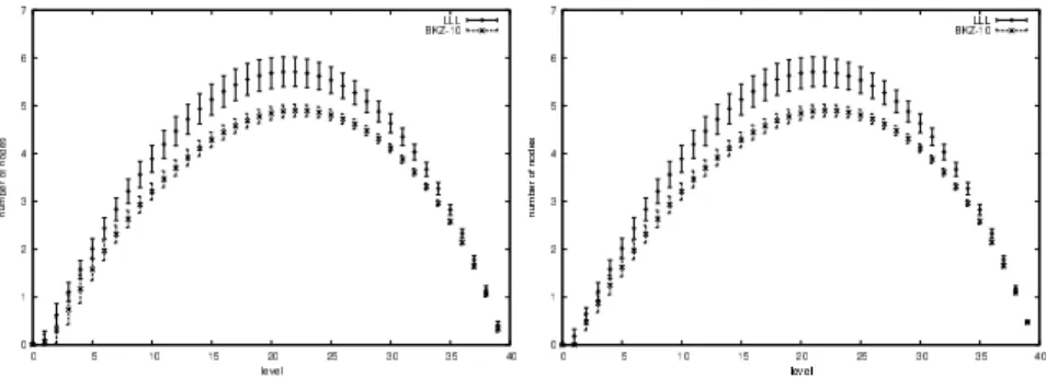
k (see [19]): the top and bottom of the tree are small, whereas the width is reached by the middle layers (it is obtained for k ≈ d/e). If the reduction is weaker, e.g., with BKZ-reduction, then the tree is even more unbalanced, with a very wide middle section, and tiny top and bottom. This is a general fact: most of the points encountered are “dead-ends” of the enumeration tree (i.e., most of the paths followed from the root end before reaching level d of the tree). We refer to Appendix A for a figure showing the number of nodes per level on typical examples.
2.3 Choosing the initial parameter A
The cost of KFP greatly depends on the initial choice for A. If the minimum λ(L) is already known, the optimal choice is A = λ(L)2. If unknown, two main
ap-proaches can be considered: use an upper bound, or start from a lower bound and increase it until a solution is found.
In the first case, an option is to set A = minikbik2. If the basis is nearly
HKZ-reduced, this might be the most efficient choice as it will be very close to λ(L)2. However, in the worst-case, the gap between min
ikbik2and λ(L) grows
with the dimension. A second option consists in using the inequality λ(L) ≤ √γ
d(det L)1/d. When the dimension is not too small, this gives a more accurate
estimate for λ(L). However, the exact values of γd are unknown in general, and
using known upper bounds on γd is likely to provide a value for A that is a
constant factor too large. If so, the cost of the enumeration will be exponentially larger than the optimal.
Another possibility consists in starting with A = minikb∗ik2, which is a lower
bound for λ(L)2. If the algorithm fails because A is too small, we try again with
a larger value of A such that the heuristic cost is multiplied by 2. As we have seen, the cost can be estimated efficiently with the Gaussian heuristic. This strategy ensures that the overall cost is no more than four times the optimal cost. Since we are mostly interested in the case where d is rather large, we may use the asymptotic lower bound γd ∼> 2πed (see [8, Ch. 1, Eq. (48)]), and
set A = d
2πe(det L)
2/d. The latter should be a rather tight estimate for λ(L)2,
for somewhat random lattices. If no solution is found for this value of A, we increase A as explained above.
3
Parallel implementation
The enumeration algorithm is typical example where the main problem can be decomposed in lots of small, independent subproblems, which pleads for a study of their parallelization. One might naively fix a level i of the tree and dispatch all subtrees with root at level i. However, the shape of the tree is not adapted to this approach: such subtasks are of too uneven a size. For instance, if the level is close to the root of the tree, the size of the largest task is of the order of magnitude of the whole computation. Furthermore, if the level i is lower, the number of tasks increases exponentially, which leads to a large number of threads, and to a quick growth of the communication cost. A better strategy is obtained by dispatching the subtasks in a dynamic way:
– Fix a computational granularity level (e.g., around 1 second); – Start the enumeration on a master machine;
– Whenever entering Step 9, estimate the cost of the corresponding subtree using the heuristic described in Section 2.2:
• if it is below the granularity level, affect this task to an available slave machine and jump to Step 13,
Note that with this strategy, there is no lower bound on the size of a task. However, each node has a small number of children (typically less than 10), which implies that a non-negligible fraction of the tasks will have a non-negligible cost. This ensures that the overall communication cost is low. If the granularity level is high, further care should be taken so that each subprocess can receive a signal whenever the value of A is updated (Step 7). Conversely, if the granularity level is sufficiently low (i.e., the communication cost is higher), it suffices to provide the new A only to the new threads.
We performed experiments to assess the accuracy of the gaussian heuristic, and refer to Appendix B for a detailed account. Typically, for d = 64, we observe that the relative error of the gaussian heuristic for any subtree whose number of nodes is more than 106 is less than 0.1%. We coded the above parallelization
technique in MPI/C++. The code achieves quasi-optimal parallelization. With a single CPU core (Intel Core 2 Quad Q9550 at 2.83 GHz), the average traversal rate is 1.27 · 107 KFP nodes per second without the recent optimisation of [13, App. D], and 1.76 · 107 with it (in dimension 64). With 10 CPU cores (plus a master which only commands the slaves), these traversal rates are multiplied by approximately 9.7.
4
Arithmetic aspects of KFP
In KFP, the quantities (µi,j, kb∗ik2, ℓi, A) are all rational, so, in theory, all
com-putations could be performed exactly. However, the bit-sizes of these numbers can be as large as Θ(d log(maxikbik)), which implies a large arithmetic
over-head. In practice, approximate arithmetic such as fixed-point or floating-point is used instead.
4.1 Fixed-point arithmetic
A fixed-point number of precision p is a real number that can be written as m · 2−pwith m ∈ Z. Any real number can be rounded to the nearest fixed-point
number with an absolute error ≤ 2−p−1. Additions and subtractions of
fixed-point numbers can be performed exactly, but the result of multiplications and divisions must be rounded. From an implementation point of view, fixed-point arithmetic is equivalent to integer arithmetic.
In software, floating-point arithmetic is more common than fixed-point arith-metic: it is standardized and available in hardware on most general-purpose CPUs, enabling reliable and efficient implementations. However, since there are no embedded floating-point operators on FPGA, and as we also want to keep the circuit as small as possible, fixed-point arithmetic is the natural choice. Addi-tionally, the resource usage of the implementation of KFP on the FPGA directly depends on the precision of the fixed-point arithmetic: The size of the data grows linearly with the precision, and the size of multipliers grows quadratically (al-though the granularity for multipliers is larger). Therefore we want to determine the smallest precision for which the result is still meaningful.
In fixed-point arithmetic, the bit-size comes from two components: the (loga-rithm of the) magnitude of the numbers we want to represent, and the precision. Here, most of the variables (xi, δxi, δ2xi, µij, and ci) have rather small
mag-nitudes. The norm kb∗
ik is not bounded, but the ratio between maxikb∗ik and
minikb∗ik is 2O(d)provided that the input is (at least) LLL-reduced and kb∗dk ≤
kb∗
1k. The LLL-reduction of the input basis can be done efficiently and we can
remove the last vector of the basis until the second condition is fulfilled (it can-not be used in an integer linear combination that leads to a shortest non-zero lattice vector). If the input basis is scaled so that 1/2 ≤ maxikb∗ik < 1, then all
variables can be represented in fixed-point arithmetic.
4.2 Numerical accuracy
The numerical behaviour of a floating-point version KFP has been studied in [40]. The main result of this article is that a precision of roughly 0.8d bits suffices to ensure the correctness when the input is LLL-reduced with quasi-optimal factors. The proof consists in bounding the magnitudes of all xi’s, yi’s and ci’s
and then analyzing the accuracy of all computations. It can readily be adapted to fixed-point arithmetic. However, for several reasons, this worst-case analysis is far from being tight for the considered lattices and bases.
A possible way to decrease the required precision, already mentioned in [40], consists in replacing the static error analysis by a dynamic algorithm which uses the exact kb∗
ik’s of the input to compute an a priori error bound for this input.
Also, as the µi,j’s and kb∗ik2’s are used many times but computed only once, we
assume that they are computed exactly and then rounded. We call this the a priori adaptive precision strategy.
Over-estimating the |xi|’s significantly contributes to the computed
suffi-cient precision being large. The bound for the |xi|’s derives from the
trian-gular inequality |P µi,jxj| ≤ P |µi,jxj|, which is very loose in practice. For
instance, on BKZ-40-reduced random knapsack lattices of dimension 64, we typ-ically obtain |xi| ≤ 226. However, the worst-case for 20 lattices of the same form
is |xi| = 54 ≤ 26. We develop the following strategy to exploit the latter
ob-servation: Let X be fixed (e.g., X = 27); We assume that |xi| ≤ X and then
bound the accuracy of ℓi; During the execution of KFP, we compare all |xi|’s
to X and check that it is valid. This strategy allows us to guarantee the validity of the computation a posteriori. In practice, this means that we have to detect overflows in the computation of |xi|’s (provided that X is set to a power of 2).
It remains to explain how to estimate the error on the ℓi’s. It can be done
via a uniform estimate (a bound of (d + 1 − i)(2Y Xd + Y2+ Y + 1)2−p−1, where
Y := (minikb∗ik)−1+ Xd ·2−p−1, can be achieved), but this leads to a significant
increase of A and/or the precision, hence of the computing time. Instead, we use the algorithm of Figure 2, which takes the above improvements into account. This gives what we call the a posteriori adaptive precision strategy.
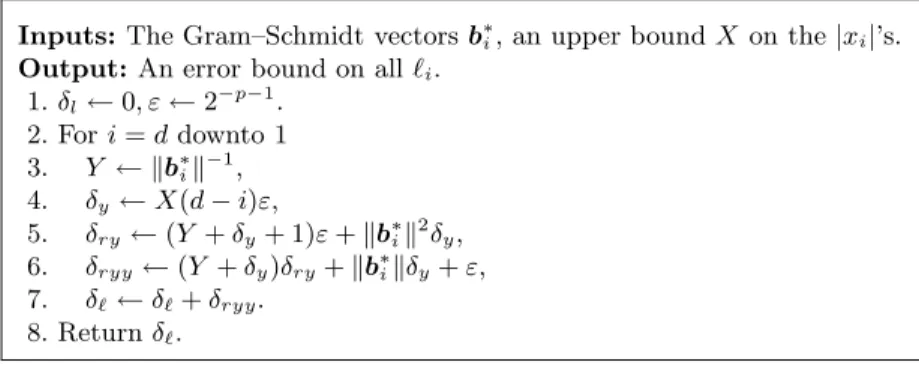
Lemma 2. The algorithm of Figure 2 (executed with rounding mode set to “to-wards +∞”) returns a valid bound for the error on all the ℓi’s.
Inputs:The Gram–Schmidt vectors b∗
i, an upper bound X on the |xi|’s.
Output:An error bound on all ℓi.
1. δl← 0, ε ← 2−p−1. 2. For i = d downto 1 3. Y ← kb∗ ik−1, 4. δy← X(d − i)ε, 5. δry← (Y + δy+ 1)ε + kb∗ik 2 δy, 6. δryy← (Y + δy)δry+ kb∗ikδy+ ε, 7. δℓ← δℓ+ δryy. 8. Return δℓ.
Fig. 2.Bounding the numerical error on the computed ℓi’s
The proof is given in Appendix C. In the examples we studied, this gave an upper bound of the order of 10−2. Once we have bounded the error on ℓ
i
by ∆max, we follow the same strategy as in [40] to compute a guaranteed solution:
add ∆max to the chosen bound A, and round it to fixed-point with rounding
towards +∞. This should be done every time A is updated.
Under the above conditions, one can prove that the shortest vector will be considered by the algorithm. However, one more modification is required if one really wants a shortest non-zero vector as an output of the algorithm: because of the errors on the ℓi’s, one might incorrectly believe that a vector b is shorter
than the current optimum b′. Hence, when Step 7 of the algorithm is entered,
the norm of b should be recomputed exactly and compared to A. Since our FPGA implementation is targeted at dealing with the intermediate levels of the enumeration tree, this computation will in practice be done in software. Note that in the context of KFP being used within BKZ, finding a vector whose norm deviates from the optimal value only because of numerical inaccuracies is deemed sufficient (see, e.g., NTL’s BKZ [47]).
In the table below, we compare the sufficient precisions we obtain with the three analyses, for several dimensions of interest. The first row gives a bound valid for any LLL-reduced basis (with the same parameters as in [40]). To com-pute the first two rows, the bound X in the algorithm is replaced by a bound which depends on i, and which is computed by using the triangular inequality and the upper bound Y . For the last row, we took X = 27, which was checked
valid in dimensions 40 and 64, and conjectured to hold for dimension 80. Each given a priori and a posteriori bound is the maximum that we obtained for 10 independent samples.
Dimension 40 64 80
Sufficient precision in the worst case 36 52 63
A priori adaptive precision 27 36 42
A posteriori adaptive precision 21 23 24
5
An FPGA-based accelerator for KFP
From the intrinsic parallelism of KFP along with its fairly limited accuracy requirements, as per Sections 3 and 4, respectively, FPGAs look like a perfectly
suitable target architecture for implementing fast and cost-efficient accelerators for short-vector enumeration in lattices. In the following, in order to assess the validity of this observation, we present the design of such an accelerator and provide the reader with performance estimations.
5.1 Choice of the target FPGA
Since we are aiming at a high-performing implementation in order to demon-strate the relevance of FPGAs as enumeration accelerators, we choose to target our implementation at a particular FPGA family. Despite losing in portability and a slightly higher design effort, this enables us to fully exploit and benefit from all the available FPGA resources.
Considering the KFP algorithm given in Figure 1, two main bottlenecks can be identified:
– first, its relatively high memory requirements: the storage necessary for the Gram–Schmidt matrix and for the local variables quickly becomes critical when considering a circuit with several KFP instances running in parallel; and
– second, the fixed-point multiplications, which are the main source of com-putations in KFP: two products need be performed at Step 5, and d − i are required to compute ciin Step 9.
Furthermore, other criteria have to be taken into account when choosing the suitable FPGA, such as the overall logic density (i.e., the number of available logic and routing elements), the achievable performance (i.e., the maximum clock frequency), and, last but not least, the actual cost of the device. Indeed, if we are to draw a fair comparison between FPGAs and CPUs when it comes to running KFP, we have to benchmark equally priced systems.
For all of the aforementioned reasons, we opted for the Xilinx Virtex-5 SXT family of FPGAs [52], and more specifically for the smallest one of the range, namely the XC5VSX35T, at the slowest speed grade (-1). For a unit price of US$460,5this FPGA combines 168 18-kbit RAM blocks, 192 DSP blocks (each
comprising a 25-by-18-bit signed multiplier and a 48-bit adder/accumulator) and 5 440 logic slices (each comprising four 6-to-1-bit look-up tables, or LUTs, and four 1-bit flip-flops), which suits reasonably well our requirements.
5.2 Main architecture of the accelerator
As the KFP enumeration algorithm lends itself quite well to parallelization, as discussed in Section 3, a natural idea to implement it in hardware is to have several small “cores” running in parallel, each one traversing a distinct subtree of the whole enumeration tree. Those subtrees are dispatched to the cores through a shared bus, and the found short vectors are collected and sent back to the host by a dedicated I/O controller.
By enumerating vectors in the corresponding subtree, each KFP core handles subproblems of fixed dimension d. We set the bound d ≤ 64, as this seems sufficient to accelerate the fat section of the enumeration tree in dimensions up to 100–120 (which is achievable with [13]). This means that the bottom layer considered in the KFP core is higher than the bottom layer of the overall tree: the subtrees possibly found below the subtree handled by the KFP core are sent back to the host and processed in software. Due to the extreme unbalanced-ness of the KFP tree, if the interval of dimensions handled by the KFP core is chosen carefully, then very few such subtrees will be found.
In the context of BKZ-type algorithms, the accelerator can be used to handle many different blocks in parallel. The BKZ blocks need not be of dimension 64: smaller dimensions can be handled on 64-dimensional KFP cores by simply set-ting the superfluous Gram–Schmidt coefficients to 0.
Finally, in order to maximize to computational power of the accelerator (which is directly proportional to the number of KFP cores that can fit on the FPGA), the resource usage of the bus and of the I/O controller should be kept as low as possible. However, since this part of the circuit is also highly dependent on the type of connectivity between the FPGA and the host, we have not implemented it yet, focusing primarily our efforts on designing efficient KFP cores.
5.3 Storing the Gram–Schmidt matrix
As previously mentioned, a critical issue of KFP lies in its memory require-ments, and more especially in the quadratic storage space required for the Gram– Schmidt matrix. Indeed, when enumerating vectors in dimension d, one needs to store all the µj,icoefficients for 1 ≤ i < j ≤ d, as all of them will take part in the
computation of the ci’s at Step 9 of the algorithm in Figure 1. This represents
d(d − 1)/2 coefficients that have to be stored on the circuit and can be accessed independently by each KFP core.
The adopted solution is also the simplest one, and is perfectly suited to low-dimensional lattices (d ≤ 64) and to memory-rich FPGAs. The idea here is to make use of the available dual-port RAM blocks on the FPGA to build a ROM for the Gram–Schmidt matrix coefficients. On the Virtex-5 FPGA we considered, those RAM blocks are 18 kbits large and can be configured as 16k×1-, 8k × 2-16k×1-, 4k × 4-16k×1-, 2k × 9- or 1k × 18-bit true dual-port memories. Additionally16k×1-, two adjacent 18-kbit blocks can be combined to form a 36-kbit RAM block, supporting from 32k × 1- to 1k × 36-bit dual-port memories. The coefficients of the Gram–Schmidt matrix can then be stored on several of such RAM blocks, their actual number depending on the required dimension d and precision p. In some case, a small amount of extra logic might also be necessary to multiplex several memories. Moreover, since the RAM blocks are dual-ported, they allow such a Gram–Schmidt matrix ROM to be shared between two KFP cores.
For instance, for a lattice of dimension d = 64 and taking p = 24 bits of precision for the µi,j’s, the ROM would require a storage capacity of d(d−1)/2 =
block (i.e., two 18-kbit blocks) configured as a 2k × 18-bit memory and one 18-kbit RAM block configured as a 2k × 9-bit memory.
5.4 Architecture of a KFP core
The basic processing unit of our accelerator is the KFP core, which runs the enu-meration algorithm depicted in Figure 1 on a subtree of the whole enuenu-meration tree. Each such core is based on a fixed-point multiplier–accumulator, which is in charge of computing the ℓi’s (Step 5) and the ci’s (Step 9). This multiplier is
coupled with a register-file responsible for storing all the local variables. Finally, a small control automaton ensures the correct execution of the algorithm, keep-ing track of the current level i and coordinates xi, δxi, and δ2xi, computing the
corresponding addresses for accessing the registered data, and multiplexing the inputs to be fed to the multiplier.
Since the overall performance of the accelerator is directly proportional to the number of KFP cores that can fit on the FPGA, it is crucial to streamline their architecture as much as possible without impacting too much on their standalone performance. To that intent, we make extensive use of the available FPGA-specific embedded features, such as DSP blocks for the fixed-point multiplier– accumulator and RAM blocks for the register file. Not only does this allow us to fully exploit most of the available resources on the FPGA, but, since these embedded blocks can usually be clocked at much higher frequencies than the logic cells, keeping the logic usage to its bare minimum is also key to designing a high-performing accelerator.
Following this rationale, the fixed-point multiplier is implemented by means of two adjacent DSP48E blocks. Thanks to their versatility, these blocks support the two modes of operation required by the KFP algorithm:
– Cascading the two DSP blocks yields a 34×24-bit unsigned multiplier, which can be used to compute successively the two products yi× kb∗ik2 and yi×
kb∗
ik2yi, for precisions p up to 24 bits. Indeed, since the bi’s are scaled (as
per Section 4.1), the squared norm kb∗
ik2 is lower than 1 and therefore fits
in p bits. Furthermore, concerning yi, 34 bits are more than enough since its
integer part, bounded by |δxi|/2, will never exceed a few bits in practice.
Finally, one can see that if kb∗
ik2yi ≥ 1 then kb∗ik2y2i ≥ 1 > A. Thus, if
the first product is greater than 1, we need not compute the second one, as ℓi will exceed the bound A and the enumeration will go up one level in the
tree. Conversely, if this product is lower than 1, then it fits on p bits and can be fed back to the multiplier in order to compute the second product. Additionally, rounding the two products to p fractional bits, along with adding ℓi+1, is achieved using the cascaded 48-bit adders available in the
DSP blocks. The comparison against the bound A is also carried out by these adders.
So as to ensure a high operating frequency, the two DSP blocks are pipelined with a latency of 3 clock cycles. Taking the cascading latency of 1 extra cycle into account, each 34 × 24-bit product is performed in 4 cycles. The
squared norm ℓi is then computed in 9 clock cycles, plus 1 additional cycle
for obtaining the difference ℓi− A.
– The computation of ci at Step 9 only requires one DSP block, configured as
a 25 × 18-bit signed multiplier–accumulator. For each product of the sum, the first operand is the p-bit Gram–Schmidt coefficient µj,i, sign-extended
to 25 bits, and the second operand is the corresponding xj, which fits in
the available 18 bits, as discussed in Section 4.2. The 48-bit accumulator embedded in the DSP block is wide enough to accommodate ciand can also
be initialized to a particular value c(0)i in order to avoid having to explicitly compute the last terms of the sum, when dealing with subtrees for which the last coordinates are fixed.
A 3-cycle-deep pipelining is also used in this mode of operation. Further-more, the products being all independent, it is possible to schedule one such product per clock cycle. The computation of ci (i.e., accumulating d − i
products) thus requires 2 + d − i clock cycles.
As far as the KFP core register file is concerned, the most suitable solution is to use an embedded 18-kbit RAM block configured as a 512 × 36-bit simple dual-port memory with independent read and write ports. The widest data to be stored in these registers are the ci’s, which have a p-bit fractional part and
an integer part the size of the xi’s. The precision p = 24 bits therefore leaves up
to 12 bits for the xi’s, which is enough in practice, as per Section 4.2.
The variables to be stored in this register file are the ℓi’s, the ci’s, the c(0)i ’s,
the triples (xi, δxi, δ2xi), the bound A, along with the constants kb∗ik2. Each
cluster of d variables is aligned on 64-word boundaries, for simpler register ad-dress computation.
Finally, as most computations and storage tasks are handled by the DSP and RAM blocks, respectively, the purpose of the control unit is mostly to feed the proper control signals to those embedded blocks. However, some computations are still directly carried out by the control unit:
– The computation of yi= |xi−ci| at Step 5 is performed by a carry-propagate
subtracter. Indeed, noticing that the sign of xi− ci is given by δ2xi, it is
possible to control the subtracter to compute either xi−cior ci−xiaccording
to the sign of δ2x
i at no additional cost.
– Updating the coordinates at Step 14 is also very efficient, provided that we use a slightly different update algorithm. Defining the variables ˜δxiand ˜δ2xi
such that ˜δxi = |δxi| and δ2xi = (−1)δ˜
2
xi, we have the following equivalent coordinate update method:
xi ← xi+ (−1) ˜ δ2
xiδx˜
i ; ˜δxi← ˜δxi+ 1 ; ˜δ2xi← NOT ˜δ2xi.
This solution is much better suited to hardware implementation, as com-puting xi± ˜δxi only requires a single adder/subtracter controlled by ˜δ2xi,
whereas computing −δxi+ δ2xi as in the original KFP algorithm involves
an extra carry propagation. Additionally, the proposed method lends itself more naturally to a parallel implementation of the three affectations.
5.5 Performance estimations
As mentioned previously, we implemented a VHDL description of our KFP accel-erator on a Xilinx Virtex-5 SXT 35 FPGA with a speed grade of -1. We present here results from the post-place-and-route area and timing estimations given by the Xilinx ISE 10.1 toolchain.
On the considered FPGA, a single KFP core designed for dimension d = 64 and precision p = 24 bits then requires 1 18-kbit RAM block, 2 DSP blocks, 274 LUTs, and 101 flip-flops (not counting the extra memory and logic used to store the Gram–Schmidt coefficients). Such a core can be clocked at an operating frequency of 250 MHz and processes a valid level-i node of the enumeration tree in 34 + d − i cycles: 20 + d − i cycles when going down to its first child and 14 cycles when coming back up from its last child. For a 64-dimensional lattice and assuming that the average node depth is 32, this yields a processing time of 264 ns per node or, equivalently, a traversal rate of 3.79 million visited nodes per second per KFP core.
It turns out that exactly 66 such cores can fit on the XC5VSX35T FPGA without lowering the clock frequency. The total resource usage is then 165 out of the 168 available 18-kbit RAM blocks (98%), 132 out of 192 DSP blocks (68%), 19 217 out of 21 760 LUTs (88%), and 6 733 out of 21 760 flip-flops (30%).6
These figures are satisfactory, as we observe a well-balanced usage of the FPGA resources: our careful design strategy, matching closely the architecture of the FPGA, really pays off at this point.
Finally, those 66 KFP cores deliver a total traversal rate of 2.50 · 108 nodes
per second. This result has however to be taken with some caution, as our imple-mentation does not take the I/O controller overhead into account. Nevertheless, we are quite confident that a carefully designed and lightweight I/O controller would not have too adverse an impact on the accelerator performance.
Of course, this rate of 2.50 · 108 traversed nodes per second is only achieved
when all of the 66 KFP cores are busy. If the main KFP problem is not properly splitted into large enough sub-instances, the cores would spend too much time performing I/Os and would therefore be completely underexploited, rendering the whole approach pointless. However, since typical dimension-64 KFP trees have several billion nodes, this should ensure keeping the communication costs negligible, even when restricted to using high-latency I/Os such as USB.
6
Conclusion
We have presented a first attempt at speeding up vector enumeration in Eu-clidean lattices by means of a dedicated FPGA accelerator. Even though the KFP algorithm lends itself particularly well to parallelization, adapting it to fully take advantage of the FPGA’s specificities requires particular care in ensuring the validity of the drastic arithmetic choices (limited precision and fixed-point
6
Actually, the FPGA is even more congested, as 5 303 out of the 5 440 available logic slices (97%) are occupied, due to some LUT/flip-flop packing issues.
instead of floating-point) and in designing the actual circuit with efficiency in mind.
The proposed accelerator achieves a cost-normalized traversal rate of 5.43·105
visited nodes per second per dollar in dimension 64, against a rate of 2.55·105for
a multi-core software implementation on an Intel Core 2 Quad Q9550 processor, thus yielding a speed-up of 2.12. The performance of our FPGA accelerator is even better compared to that of the GPU implementation proposed in [20] which delivers a total traversal rate of 1.36 · 105nodes per second per dollar.
All in all, it appears that, thanks to our implementation, FPGAs qualify as a perfectly relevant architecture for accelerating lattice reduction, thus calling for further investigations in that direction.
Acknowledgments. The authors would like to thank Jens Hermans and Michael Schneider for helpful discussions, the anonymous reviewers for their valuable comments, and Florent de Dinechin for fruitful discussions when this work was initiated. The last author was partly supported by the ARC Discovery Grant DP0880724 “Integral lattices and their theta series”.
References
1. Agrawal, S., Boneh, D., Boyen, X.: Efficient lattice (H)IBE in the standard model (2010), to appear in the proceedings of Eurocrypt 2010
2. Ajtai, M.: The shortest vector problem in L2is NP-hard for randomized reductions
(extended abstract). In: Proc. of STOC. pp. 284–293. ACM (1998)
3. Ajtai, M., Dwork, C.: A public-key cryptosystem with worst-case/average-case equivalence. In: Proc. of STOC. pp. 284–293. ACM (1997)
4. Ajtai, M., Kumar, R., Sivakumar, D.: A sieve algorithm for the shortest lattice vector problem. In: Proc. of STOC. pp. 601–610. ACM (2001)
5. Arbitman, Y., Dogon, G., Lyubashevsky, V., Micciancio, D., Peikert, C., Rosen, A.: SWIFFTX: a proposal for the SHA-3 standard. Submission to NIST (2008), http://www.eecs.harvard.edu/~alon/PAPERS/lattices/swifftx.pdf
6. Cad´e, D., Pujol, X., Stehl´e, D.: fplll - a floating-point LLL implementation, avail-able at http://perso.ens-lyon.fr/damien.stehle
7. Cash, D., Hofheinz, D., Kiltz, E., Peikert, C.: Bonsai trees, or how to delegate a lattice basis (2010), to appear in the proceedings of Eurocrypt 2010
8. Conway, J.H., Sloane, N.J.A.: Sphere Packings, Lattices and Groups. Springer (1988)
9. Coppersmith, D.: Small solutions to polynomial equations, and low exponent RSA vulnerabilities. J. Cryptology 10(4), 233–260 (1997)
10. van Dijk, ., Gentry, C., Halevi, S., Vaikuntanathan, V.: Fully homomorphic en-cryption over the integers (2010), to appear in the proceedings of Eurocrypt 2010 11. Fincke, U., Pohst, M.: A procedure for determining algebraic integers of given
norm. In: Proc. of EUROCAL. LNCS, vol. 162, pp. 194–202. Springer (1983) 12. Gama, N., Nguyen, P.Q.: Finding short lattice vectors within Mordell’s inequality.
In: Proc. of STOC. pp. 207–216. ACM (2008)
13. Gama, N., Nguyen, P.Q., Regev, O.: Lattice enumeration using extreme pruning (2010), to appear in the proceedings of Eurocrypt 2010
14. Gentry, C.: Fully homomorphic encryption using ideal lattices. In: Proc. of STOC. pp. 169–178. ACM (2009)
15. Gentry, C., Peikert, C., Vaikuntanathan, V.: Trapdoors for hard lattices and new cryptographic constructions. In: Proc. of STOC. pp. 197–206. ACM (2008) 16. Goldreich, O., Goldwasser, S., Halevi, S.: Public-key cryptosystems from lattice
reduction problems. In: Proc. of CRYPTO. LNCS, vol. 1294, pp. 112–131. Springer (1997)
17. Goldstein, D., Mayer, A.: On the equidistribution of Hecke points. Forum Mathe-maticum 15, 165–189 (2003)
18. Guo, Z., Nilsson, P.: VLSI architecture of the soft-output sphere decoder for MIMO systems. In: Proc. of MWSCAS. vol. 2, pp. 1195–1198. IEEE (2005)
19. Hanrot, G., Stehl´e, D.: Improved analysis of Kannan’s shortest lattice vector algo-rithm. In: Proc. of CRYPTO. LNCS, vol. 4622, pp. 170–186. Springer (2007) 20. Hermans, J., Schneider, M., Buchmann, J., Vercauteren, F., Preneel, B.:
Parallel shortest lattice vector enumeration on graphics cards. In: Proc. of AFRICACRYPT. LNCS, vol. 6055, pp. 52–68. Springer (2010)
21. Hoffstein, J., Pipher, J., Silverman, J.H.: NTRU: A ring-based public key cryp-tosystem. In: Proc. of ANTS. pp. 267–288 (1998)
22. Howgrave-Graham, N.: A hybrid lattice-reduction and meet-in-the-middle attack against NTRU. In: Proc. of CRYPTO. LNCS, vol. 4622, pp. 150–169. Springer (2007)
23. Kannan, R.: Improved algorithms for integer programming and related lattice prob-lems. In: Proc. of STOC. pp. 99–108. ACM (1983)
24. Lenstra, A.K., Lenstra, Jr., H.W., Lov´asz, L.: Factoring polynomials with rational coefficients. Math. Ann. 261, 515–534 (1982)
25. Lov´asz, L.: An Algorithmic Theory of Numbers, Graphs and Convexity. SIAM (1986), cBMS-NSF Regional Conference Series in Applied Mathematics
26. Magma: The Magma computational algebra system, available at http://magma. maths.usyd.edu.au/magma/
27. May, A.: Using LLL-reduction for solving RSA and factorization problems: A sur-vey (2009), chapter of [32]
28. Micciancio, D., Regev, O.: Lattice-based cryptography. In: Post-Quantum Cryp-tography, D. J. Bernstein, J. Buchmann, E. Dahmen (Eds). pp. 147–191. Springer (2009)
29. Micciancio, D., Voulgaris, P.: A deterministic single exponential time algorithm for most lattice problems based on Voronoi cell computations (2010), to appear in the proceedings of STOC 2010
30. Micciancio, D., Voulgaris, P.: Faster exponential time algorithms for the shortest vector problem. In: Proc. of SODA. pp. 1468–1480. SIAM (2010)
31. Mow, W.H.: Maximum likelihood sequence estimation from the lattice viewpoint. IEEE TIT 40, 1591–1600 (1994)
32. Nguyen, P.Q., (Eds), B.V.: The LLL algorithm, survey and applications. Informa-tion Security and Cryptography, Springer (2010)
33. Nguyen, P.Q., Stehl´e, D.: Floating-point LLL revisited. In: Proc. of EUROCRYPT. LNCS, vol. 3494, pp. 215–233. Springer (2005)
34. Nguyen, P.Q., Stehl´e, D.: LLL on the average. In: Proc. of ANTS. LNCS, vol. 4076, pp. 238–256. Springer (2006)
35. Nguyen, P.Q., Stern, J.: Cryptanalysis of the Ajtai-Dwork cryptosystem. In: Proc. of CRYPTO. LNCS, vol. 1462, pp. 223–242. Springer (1998)
36. Nguyen, P.Q., Stern, J.: The two faces of lattices in cryptology. In: Proc. of CALC. LNCS, vol. 2146, pp. 146–180. Springer (2001)
37. Nguyen, P.Q., Vidick, T.: Sieve algorithms for the shortest vector problem are practical. J. Mathematical Cryptology 2(2) (2008)
38. Odlyzko, A.M.: The rise and fall of knapsack cryptosystems. In: Proceedings of Cryptology and Computational Number Theory. Proceedings of Symposia in Ap-plied Mathematics, vol. 42, pp. 75–88. AMS (1989)
39. Peikert, C.: Public-key cryptosystems from the worst-case shortest vector problem. In: Proc. of STOC. pp. 333–342. ACM (2009)
40. Pujol, X., Stehl´e, D.: Rigorous and efficient short lattice vectors enumeration. In: Proc. ASIACRYPT. LNCS, vol. 5350, pp. 390–405. Springer (2008)
41. Pujol, X., Stehl´e, D.: Solving the shortest lattice vector problem in time 22.465n.
Cryptology ePrint Archive, Report 2009/605 (2009), http://eprint.iacr.org/ 2009/605
42. Regev, O.: Lattices in computer science (2004), lecture notes of a course given at the Tel Aviv University. Available at http://www.cs.tau.ac.il/~odedr/teaching/ lattices_fall_2004/
43. Regev, O.: On lattices, learning with errors, random linear codes, and cryptogra-phy. In: Proc. of STOC. pp. 84–93. ACM (2005)
44. Schnorr, C.P.: A hierarchy of polynomial lattice basis reduction algorithms. Theor. Comput. Sci 53, 201–224 (1987)
45. Schnorr, C.P., Euchner, M.: Lattice basis reduction: improved practical algorithms and solving subset sum problems. Math. Programming 66, 181–199 (1994) 46. Schnorr, C.P., H¨orner, H.H.: Attacking the Chor-Rivest cryptosystem by improved
lattice reduction. In: Proc. of EUROCRYPT. LNCS, vol. 921, pp. 1–12. Springer (1995)
47. Shoup, V.: NTL, Number Theory C++ Library, available at http://www.shoup. net/ntl/
48. Smart, N.P., Vercauteren, F.: Fully homomorphic encryption with relatively small key and ciphertext sizes (2010), to appear in the proceedings of PKC 2010 49. Stehl´e, D., Steinfeld, R., Tanaka, K., Xagawa, K.: Efficient public key encryption
based on ideal lattices. In: Proc. of ASIACRYPT. LNCS, vol. 5912, pp. 617–635. Springer (2009)
50. Studer, C., Burg, A., B¨olcskei, H.: Soft-output sphere decoding: Algorithms and VLSI implementation. IEEE Journal on Selected Areas in Communications 26(2), 290–300 (2008)
51. Viterbo, E., Boutros, J.: A universal lattice code decoder for fading channels. IEEE TIT 45, 1639–1642 (1999)
52. Xilinx: Virtex-5 family overview, available at http://www.xilinx.com/support/ documentation/virtex-5.htm
A
Shape of the KFP tree
In Figures 3, 4, we compare the Gaussian approximation and the actual number of KFP-nodes per level on the same type of bases, using similar reductions. Note that for dimension 64, only the BKZ-40 preprocessing allows for enumeration in a reasonable amount of time, explaining the fact that the left graphics only has one curve.
Fig. 3.Number of nodes per level in KFP, dimension 40: experimental (left), Gaussian estimate (right)
Fig. 4.Number of nodes per level in KFP, dimension 64: experimental (left), Gaussian estimate (right)
B
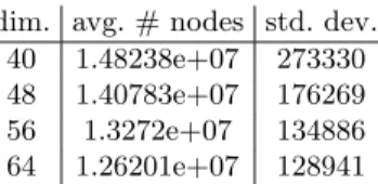
Performance of the software implementation of KFP
The tables below give the number of nodes treated per second of our software im-plementations of the KFP algorithm on an Intel Core 2 Quad Q9550 at 2.83 GHz, with or without the optimization described in [13, App. D]. These data have been obtained via the enumeration of 32 different lattices; we provide the average number of nodes per second and the standard deviation.
We also provide data regarding parallelization. The granularity level has been set to 2 · 107 nodes. The left diagram shows the number of subtrees of the
enumeration that have (estimated via the Gaussian heuristic) size ≤ 2 · 107 and whose father has (estimated) size > 2 · 107; we call these subtrees slave subtrees.
The right diagram shows that the Gaussian heuristic remains extremely reliable in this context: for 95% of trees of size 215, it estimates the correct size within
a factor < 1.01.
The latter shows that the size of tasks is rather well estimated (mainly, no “large” subtree is mistakenly handled as a small one), whereas the former shows
dim. avg. # nodes std. dev. 40 1.48238e+07 273330 48 1.40783e+07 176269 56 1.3272e+07 134886 64 1.26201e+07 128941
dim. avg. # nodes std. dev. 40 1.72778e+07 281925 48 1.73586e+07 96808.5 56 1.74355e+07 127681 64 1.75637e+07 179223 Fig. 5. Number of nodes per second in software, unoptimized version (left) versus optimized (right)
Fig. 6.Left: number of unique subtrees of a given size; right: validity of the Gaussian approximation as a function of tree size
that most of the tasks below a given granularity level are in fact of size close to that granularity level: the parallelization proposed is extremely close to splitting the tree into pieces of equal sizes.
C
Proof of Lemma 2
For any quantity α, we denote its fixed-point evaluation by ¯α. We also de-fine ∆α = |α − ¯α|. Let ε = 2−p−1, where p is the precision of the fixed-point
arithmetic. The Gram–Schmidt coefficients can be computed exactly in software and then rounded, which ensures that ∆µi,j≤ ε and ∆(kb∗ik2) ≤ ε.
This implies that ∆yi≤ (d − i − 1)Xε. We now consider an iteration of KFP
where ℓi≤ A (≤ 1). This implies that yi≤ kb∗ik−1, which gives kb∗ik2yi≤ kb∗ik
and ¯yi≤ kb∗ik−1+ ∆yi. The product kb∗ik2yi2 is computed as (kb∗ik2× yi) × yi,
and we thus bound the error on this product in two steps: ∆(riyi) ≤ ε + ¯yiε + ri∆yi,
∆(riyi2) ≤ ε + ¯yi∆(yiri) + riyi∆yi.
Finally, for all i we have ∆ℓi ≤Pdj=i∆(rjyj2). The correctness of the