HAL Id: tel-01801799
https://tel.archives-ouvertes.fr/tel-01801799
Submitted on 28 May 2018
HAL is a multi-disciplinary open access archive for the deposit and dissemination of sci-entific research documents, whether they are pub-lished or not. The documents may come from teaching and research institutions in France or abroad, or from public or private research centers.
L’archive ouverte pluridisciplinaire HAL, est destinée au dépôt et à la diffusion de documents scientifiques de niveau recherche, publiés ou non, émanant des établissements d’enseignement et de recherche français ou étrangers, des laboratoires publics ou privés.
complex systems
Yueying Zhu
To cite this version:
Yueying Zhu. Investigation on uncertainty and sensitivity analysis of complex systems. General Physics [physics.gen-ph]. Université du Maine, 2017. English. �NNT : 2017LEMA1021�. �tel-01801799�
Yueying ZHU
Mémoire présenté en vue de l’obtention du
grade de Docteur de Le Mans Université
sous le sceau de l’Université Bretagne Loire
École doctorale : 3M Discipline : Physique
Spécialité : Atomes, Molécules et Plasmas Unité de recherche : IMMM
Soutenue le 23 Octobre 2017 Thèse N° :
Investigation on uncertainty and sensitivity
analysis of complex systems
JURY
Rapporteurs : Jérôme MORIO, Professeur, ONERA
Olivier LE MAITRE, Professeur, CNRS, LIMSI
Examinateurs : Benoît ROBYN, Professeur, HEI-Yncréa Hauts de France
Marina KLEPTSYNA, Professeur, Le Mans Université Michel BASSET, Professeur, Université de Haute Alsace (UHA) Wei LI, Professeur, Central China Normal University
Directeur de Thèse : Q. Alexandre WANG, Professeur, Ecole Hautes Etudes Ingénieurs et Le Mans Université Co-directeur de Thèse : Alain BULOU, Professeur CNRS, IMMM- Le Mans Université
By means of taylor series expansion, a general analytic formula is derived to characterise the uncertainty propagation from input variables to the model response, in assuming input independence. By using power-law and exponential functions, it is shown that the widely used approximation considering only the first order contribution of input uncertainty is sufficiently good only when the input uncertainty is negligible or the underlying model is almost linear. The method is then applied to a power grid system and the EOQ model.
The method is also extended to correlated case. With the extended method, it is s-traightforward to identify the importance of input correlations in the model response. This allows one to determine whether or not the input correlations should be considered in practical applications. Numerical examples suggest the effectiveness and validation of our method for general models, as well as specific ones such as the deterministic HIV model.
Our method is then compared to Sobol’s one which is implemented with sampling based strategy. Results show that, compared to our method, it may overvalue the roles of individual input factors but underestimate those of their interaction effects when there are nonlinear coupling terms of input factors. A modification is then introduced, helping understand the difference between our method and Sobol’s one.
Finally, a numerical model is designed based on a virtual gambling mechanism, regarding the formation of opinion dynamics. Theoretical analysis is proposed by the use of one-at-a-time method. Sampling-based method provides a global analysis of output uncertainty and sensitivity.
Keywords: Uncertainty analysis, Sensitivity analysis, Variance decomposition, Sam-pling, Correlation, Sensitivity measure, Opinion dynamics
Par un d´eveloppement en s´erie de Taylor, une relation analytique g´en´erale est ´etablie pour calculer la propagation des incertitudes des variables d’entr´ee sur la r´eponse du mod`ele, en assumant l’ind´ependance des entr´ees. En utilisant des relations puissances et des relations exponentielles, il est d´emontr´e que l’approximation souvent utilis´ee con-sistant `a ne consid´erer que la contribution du premier ordre sur l’incertitude d’entr´ee permet d’´evaluer de mani`ere satisfaisante l’incertitude sur la r´eponse du mod`ele pourvu que l’incertitude d’entr´ee soit n´egligeable ou que le mod`ele soit presque lin´eaire. La m´ethode est appliqu´ee `a l’´etude d’un r´eseau de distribution ´electrique et `a un mod`ele d’ordre ´economique.
La m´ethode est ´etendue aux cas o`u les variables d’entr´ee sont corr´el´ees. Avec la m´ethode g´en´eralis´ee, on peux d´eterminer si les corr´elations d’entr´ee doivent ou non ˆetre consid´er´ees pour des applications pratiques. Des exemples num´eriques montrent l’efficacit´e et la validation de notre m´ethode dans l’analyse des mod`eles tant g´en´eraux que sp´ecifiques tels que le mod´ele d´eterministe du VIH.
La m´ethode est ensuite compar´ee `a celle de sobol. Les r´esultats montrent que la m´ethode de sobol peut sur´evaluer l’incidence des divers facteurs, mais sous-estimer ceux de leurs interactions dans le cas d’interactions non lin´eaires entre les param`etres d’entr´ee. Une modification est alors introduite, aidant `a comprendre la diff´erence entre notre m´ethode et celle de sobol.
Enfin, un mod´ele num´erique est ´etabli dans le cas d’un jeu virtuel prenant en compte la formation de la dynamique de l’opinion publique. L’analyse th´eorique `a l’aide de la m´ethode de modification d’un param`etre `a la fois. La m´ethode bas´ee sur l’´echantillonnage fournit une analyse globale de l’incertitude et de la sensibilit´e des observations.
Mots-cl´es: Analyse d’incertitude, Analyse de sensibilit´e, D´ecomposition de variance, Echantillonnage, Corr´elation, Mesure de sensibilit´e, Dynamique d’opinion
My Ph.D. study of three years is near its ending. I was continuously supported and encouraged by my supervisors, colleagues, friends, and family members. At this special and important moment, I would like to express my sincere gratitude to all of them. First and foremost, I would like to show the greatest appreciation to my supervisor, Prof. Q. Alexandre Wang, who provided me an exciting opportunity to study in France, particularly, in ISMANS at the beginning and then at Le Mans University. He guided me to a more international research environment and also offered me a special platform to communicate and discuss with scholars from different fields and countries. It has been a great honor to be one of his Ph.D. students. I deeply appreciate his continuous support, innovative ideas, valuable suggestions and timely guidance, which all are useful and beneficial to my Ph.D. study and related research, and also make my study experience productive and stimulating. The tremendous interests and enthusiasm he has for his research, as well as his immense knowledge, are contagious and motivational for me, even during tough times in the Ph.D. pursuit. I am also grateful for the great help that he and his wife offered for my daily life in France.
I am especially thankful to my supervisor, Prof. Xu Cai, working at Central China Normal University. He introduced me to the research filed of Complexity Science and provided me many chances to attend international academic conferences. He encouraged me to persistently move forward and to work independently. As a mentor, except for the knowledge related to research, he also taught me how to positively face setbacks in study and life, how to communicate with others, how to build good personality, how to ”conduct oneself”, etc. His encouragement and unlimited support incented me to do better both in study and life.
My sincere thanks also go to Prof. Wei Li, my another supervisor working at Central China Normal University. He guided me to do numerical simulations and theoretical analysis. He taught me how to write a research paper, how to reply the referee’s report, etc. I am particularly indebted to him for his constant encouragement and endless support throughout the whole stage of my postgraduate study. His insightful comments and valuable ideas have particularly contributed to the writing of this thesis.
I would like to thank my associate supervisor, Prof. Alain Bulou, for his constant encouragement and support when I studied at IMMM. He provided me financial support to attend a particular international academic conference, and permission to use facilities of the laboratory. He is very gentle and always offers help to me when I am in troubles.
I would also like to thank the rest members of my thesis committee: Prof. Olivier Le Maˆıtre, Prof. J´erˆome Morio, Prof. Benoˆıt Robyns, Prof. Marina Kleptsyna, and Prof. Michel Basset, for their insightful comments and hard questions which stimulate me to extend my research from various perspectives.
I am hugely appreciative to Prof. Liping Chi from Central China Normal University. She introduced me to the interesting research field of public opinion dynamics at the beginning of my master study. She is more like a sister who always encourages and cares for me. Special mention should also go to her generous assistance in polishing the thesis. Profound gratitude goes to Prof. Chunbin Yang at Central China Normal University for his helpful discussions about theoretical analysis. Gratitude also goes to Profs. Wenping Bi and Paul Bourgine, the CST external scientific members, for their insightful reports and comments about my study progress. Special thanks should be expressed to Prof. Jean-Marc Greneche, for his support, encouragement, and warm assistance both in academic research and daily life, to Prof. Florent Calvayrac, for his consideration to my study and valuable suggestions about providing an oral presentation, and to Francis Chavanon, for his kind help in using the server machine of the laboratory.
I would especially like to thank Sa¨ıda M´enard. It is quite hard to study alone in a foreign country. As my best friend in France, she consorted with me for numerous moments of helplessness and loneliness. I am deeply indebted to her for the persistent support, encouragement, contribution of time, and anything else she did for me in daily life. I would also like to thank Mich`ele Houdusse, my reception family in France, for her kind help and consideration during my stay here.
Sincere thanks also go to my colleagues and other friends in Le Mans: Anna Kharlamova, Fan Wang, Lei Xiong, Liyang Zheng, Lizhong Zhao, Ru Wang, Van Tang Nguyen and Wenting Guo, for all the fun and pleasure we have had within the last three years; and to all the previous and current members in Complexity Science Center of Central China Normal University, for their constant support, warm assistance, and productive discussions. In particular, I am grateful to Dr. Jian Jiang for his valuable comments in the writing of the thesis.
I gratefully acknowledge the financial support that enabled me to finish smoothly my Ph.D. study in France. I was funded by China Scholarship Council. My work was also partially supported by the Programme of Introducing Talents of Discipline to Universi-ties of China, the National Natural Science Foundation of China, the Ecole Doctorale 3M at Le Mans University, and the Institut des Mol´ecules et Mat´eriaux du Mans (IMMM). Last but not the least, I would like to take this opportunity to express my deepest appreciation to my parents, parents-in-law, brother, sister-in-law, nephew and niece, for
their selfless love in my life, continuous support and encouragement in all my pursuits. And most of all, I wish to thank my husband, for his faithful love, constant support, unconditional pay, trust, and understanding during the stage of my Ph.D. study in France.
Le Mans, France October, 2017
Abbreviations
AIDS Acquired Immune Deficiency Syndrome CC Pearson Correlation Coefficient
CCDF Complementary Cumulative Distribution Function CDF Cumulative Distribution Function
CL2 Centered L2-discrepancy
EOQ Economic Order Quantity
HIV Human Immunodeficiency Virus
IFFD Iterated Fractional Factorial Design KRCC Kendall Rank Correlation Coefficient LHS Latin Hypercube Sampling
MC Monte Carlo
PCC Partial Correlation Coefficient PDF Probability Density Function
PRCC Partial Rank Correlation Coefficient
QMC Quasi Monte Carlo
RCC Rank Correlation Coefficient SIR Susceptible-Infected-Recovered SIS Susceptible-Infected-Susceptible
Abstract i R´esum´e ii Acknowledgements iii Abbreviations vi General introduction 1 1 Introduction 4
1.1 Characterisation of uncertainty in model input . . . 6
1.2 Presentation of uncertainty in model output . . . 8
1.3 Methods of sensitivity analysis . . . 11
1.3.1 One-at-a-time method . . . 12
1.3.2 Regression analysis method . . . 14
1.3.3 Response surface method . . . 16
1.3.4 Differential-based method . . . 20
1.3.5 Variance-based methods . . . 22
1.3.6 Moment independent method . . . 25
1.3.7 Sampling-based method . . . 26
1.4 Determination of analysis results . . . 35
1.4.1 Scatter plots . . . 35
1.4.2 Correlation measures. . . 39
1.4.3 Sensitivity indices . . . 43
2 The analytic analysis for models with independent input variables 48 2.1 Taylor series. . . 48
2.2 Variance propagation for univariate case . . . 49
2.2.1 Uniform distribution . . . 51
2.2.2 Normal distribution . . . 53
2.3 Generalisation of the analytic formula . . . 55
2.4 Applications to the analysis of complex systems . . . 56
2.4.1 Power grid system . . . 57 vii
2.4.2 Economic system . . . 61
3 The analytic analysis for models with correlated input variables 64 3.1 Variance propagation. . . 64
3.2 Estimation of sensitivity indices . . . 66
3.2.1 Generation of correlated variables . . . 67
3.2.2 Sensitivity indices . . . 69
3.3 Numerical examples and a practical application . . . 72
3.3.1 Additive linear model . . . 72
3.3.2 Nonlinear models . . . 73
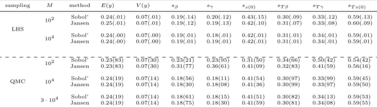
4 The establishment of sampling-based strategy 83 4.1 A comparison of our method with Sobol’s one . . . 83
4.2 Analysis of SIR and SIS models . . . 86
5 Opinion formation based on a gambling mechanism and its sensitivity analysis 91 5.1 Introduction. . . 91
5.2 Modeling . . . 93
5.3 Methods . . . 95
5.4 Results and discussion . . . 96
5.4.1 Theoretical analysis for special cases . . . 97
5.4.2 The distribution of Ωs in general situations . . . 103
5.4.3 Opinion Clustering . . . 106
5.4.4 The fraction of winners . . . 107
5.4.5 Uncertainty and Sensitivity analysis . . . 109
6 Conclusions and Prospectives 111 6.1 Conclusions . . . 111
6.2 Future work plan . . . 113
A Central moments 115 A.1 Uniform distribution . . . 115
A.2 Normal distribution . . . 116
B Generation of correlated variables 117 B.1 Two correlated variables . . . 117
B.2 Three correlated variables . . . 118
B.3 Four correlated variables . . . 119
C Derivation of Eqs. (3.51-3.52) 121 C.1 First-order contributions . . . 121
C.2 Second-order contributions . . . 123
C.3 Third-order contributions . . . 124
D Derivation of the fourth-order central moment with four different
E Partial variance contributions for Ishigami function 128
E.1 First-order contributions . . . 128
E.2 Second-order contributions . . . 130
F Special case for opinion formation: p = γ = 0 134
Bibliography 139
The concept of global uncertainty and sensitivity analysis has proposed for a long time. It attracts the considerations of a large number of researchers from various of areas. The global uncertainty and sensitivity analysis aims at analysing the uncertainties of output variables (also called observations or model responses) according to the uncertainties in input variables (or named factors, parameters, covariates), and the sensitivity of each output variable with respect to individual input parameters, as well as to their inter-actions. Undoubtedly, global uncertainty and sensitivity analysis is advantageous for gaining insight into how input variables should be ranked according to their importance in establishing the uncertainties in different output variables. While the strategies for uncertainty and sensitivity analysis are quite extensive, a general analytic method is still limited, especially for models of present input correlations. In this dissertation, we main-ly focus on the establishment of a general theoretical framework for global uncertainty and sensitivity analysis in the modelling of complex systems.
Mathematical models have a wide range of applications in diverse disciplines. They can help explain a system by visualized data and/or figures and analyse the possible effects of different parameters, and also, if necessary, make predictions about the underlying behaviour. With a deterministic mathematical model of general form y = f (x) with y denoting the output vector and x indicating the input vector. When y is calculated from x through a specified function or some natural or artificial rules connecting y and x, uncertainties in the elements of input vector, if exist, will propagate through the calculation to the members of output vector y dependent on x [1, 2]. This process is called variance propagation (or uncertainty propagation). Variance propagation, often regarded as the fundamental ingredient of sensitivity analysis for complex models, mainly considers the determination of output’s variance via uncertainties in input factors [3,4]. At present, many strategies have been built for the determination of variance propa-gation, such as simulation-based methods[5, 6], most probable point-based methods[7,
8], functional expansion-based methods[9], numerical integration-based methods[10–13]. Simulation-based methods, also called sampling-based methods, are regarded as both
effective and widely used, especially for those models with the functional relationship connecting y and x absent [14–16]. These briefly mentioned strategies, however, are computationally expensive, especially in the presence of a high number of input vari-ables. For a general model with given functional form, the procedure will be much easier and numerically cheaper for determining the output’s variance if an analytic formula as-sociated with variance propagation can be provided. More information asas-sociated with other methods for variance propagation can be found in some reviewed papers [17–19]. A simple analytic formula has been appeared since 1953. It approximately computes the variance of the product of two independent random variables [20]. In 1966, this approximation was extended by engineers and experimentalists to more general multi-variate cases [21]. This formula, also called Taylor series approximation, restricted to the first-order terms [22], has gained a wide applications thanks to its simplicity and convenience [23]. However, it can satisfactorily estimate the output’s variance only when the functional relationship between output and input variables is almost linear or the uncertainty of each input variable is negligible [17]. For most models, y highly nonlin-early depends on x having large uncertainties. This suggests the necessity of an exact analytic formula in calculating the output’s variance and evaluating its sensitivities with respect to individual input factors, as well as to their interactions.
Furthermore, many methods have also been designed for performing sensitivity analy-sis, including the traditional approach of changing one factor at a time [24, 25], local method [26], regression analysis [27], variance-based method [28], etc. Among the vari-ous available strategies, variance-based sensitivity analysis has been assessed as versatile and effective for uncertainty and sensitivity analysis of model response. The considera-tion of variance-based importance measures can be traced back to over twenty years ago when Sobol characterised the first-order sensitivity measures on the basis of deposing the variance in model response into different partial contributions attributable to individual input variables and to their combinations (called variance decomposition) [29]. Then extensive relevant investigations are carried out around this Sobol’s work, boiling down to the improvements in analysis strategies and to their applications to the sensitivity and reliability analysis of complex systems [30,31]. However, these frameworks, as well as above mentioned strategies for the determination of variance propagation, are often proposed when the input variables are assumed to be statistically independent.
Recently, the interest in extending sensitivity analysis strategies from uncorrelated case to the correlated one is increasing as correlated factors are often happened in practical applications. Previous investigations about sensitivity analysis of models in the presence of input correlations only provided overall sensitivity indices with respect to individual input factors. However, the correlated and independent variance contributions were
absent [32]. In practical applications, the distinction between independent and correlated contributions is quite important. It allows one to decide whether or not the correlations among input factors should be considered.
Both correlated and independent variance contributions were firstly considered by C. Xu et al [33]. They proposed a regression-based strategy to decompose partial variance contributions into independent and correlated parts by assuming approximate linear dependence between model response and input variables. To overcome the limitation of their method, many frameworks on sensitivity analysis are recently developed in the presence of input correlations, contraposing the investigation of more effective and universal technics for sensitivity analysis in general correlated situations [34–36]. Still, a theoretical framework of the determination of partial variance contributions and of relative correlated and independent effects is limited, especially when a single input is correlated with many others simultaneously.
Consequently, in this dissertation, we mainly focus on the establishment of a theoretical framework for uncertainty and sensitivity analysis. The applications of sampling-based method are also proposed to the uncertainty and sensitivity analysis of epidemic spread-ing and opinion formation systems.
The manuscript is organised as follows. The first chapter introduces in detail the back-ground of uncertainty and sensitivity analysis of complex systems. It also provides the implementation of uncertainty and sensitivity analysis by using different strategies. In the second chapter, a systematic theoretical framework is established for the uncertainty and sensitivity analysis of general models with given functional forms, by assuming that input factors are statistically independent of each other. In the third chapter, the the-oretical method for uncertainty and sensitivity analysis is generalised to more universal models of input correlations. The fourth chapter concerns the difference of our method from Sobol’s one. A rough sampling-based approach that is coincident with our analyt-ic method is then established by introducing a modifanalyt-ication to the Sobol’s method, in assuming input independence. A systematic framework on uncertainty and sensitivity analysis of a numerical model is described in chapter 5. This model considers the for-mation of public opinion dynamics based on a virtual gambling mechanism. Finally, a general conclusion and future work plan are given.
Introduction
Mathematical models are of great importance in the natural sciences. They have been diffusely utilized in many disciplines as diverse as mathematics [37,38], physics [24,25,
39–42], chemistry [43], etc. With mathematical models, one can explicate a system in mathematical language, analyse the roles of linked factors by physical methods, and then make reasonable predictions of underlying behaviors. In general a model contains three major elements: the input vector, the output vector, and associations between them. In practical applications, the elements of input vectors are rarely deterministic but contain uncertainty following some distribution laws [44, 45]. Consequently, the determination of the variations in input variables, the investigation of their propagating through the model, as well as the quantification of the sensitivities of model outputs with respect to input variables are of crucial importance for establishing reliable and robust models [3, 33, 46, 47]. The implementation of these procedures is known as uncertainty and sensitivity analysis.
A view of modeling that may help illustrate the role of uncertainty and sensitivity analysis in the scientific process is offered in Fig. 1.1, taken from the work of Robert Rosen, an American theoretical biologist [48]. The figure shows two systems, a natural system N which forms the subject under investigation, and a formal system F which indicates the modeling of this subsect. Each system has its own internal entailment structures and the two systems are connected by the encoding and decoding processes. The uncertainty under discussion here is often referred to as epistemic uncertainty (also known as systematic uncertainty). Epistemic uncertainty derives from a lack of infor-mation or non-accuracy in measurement about the appropriate value used for specifying a quantity that is assumed to be constant in the context of the analysis for a particular problem. In the conceptual and computational designation of an analysis, epistemic uncertainty is regarded in general to be distinct from aleatory uncertainty, which, also
Figure 1.1: Modeling after Rosen (1991)
known as statistical uncertainty, arises from an inherent randomness in the behavior of the system under study.
Uncertainty and sensitivity analysis are essential parts of analyses for complex systems. Specifically, sensitivity analysis considers the determination of variance contributions of individual input variables to the elements of output vectors [49]. Uncertainty analysis, preceding sensitivity analysis, mainly focuses on the determination of the uncertainties in output variables that derive from uncertainties in input factors. Conceptually, un-certainty and sensitivity analyses should be run in tandem. They work together to help determine:
(1) Which input factors contribute most to the variation of model output.
(2) Which parameters are significant and which ones can be eliminated from the model; (3) How to efficiently reduce the uncertainty in model output by strengthening the knowledge base concerning input parameters.
Quantifying the impact of a variable under sensitivity analysis could be useful for a series of purposes, such as deep understanding of the relationships between input and output variables in a system or model, fixing model inputs that have no effect on the output, identifying and removing redundant parts of the model structure, and avoiding useless time consumption on non-sensitive variables in models of a large number of parameters. In models consisting of a large number of input variables, sensitivity analysis constitutes essential ingredient of model building and quality assurance. Sensitivity analysis has also extended its application to national and international agencies involved in impact assessment studies, including the European Commission [50,51], Australian pathology laboratories [52], the Intergovernmental Panel on Climate Change [53], and US Environmental Protection Agency’s modelling guidelines [54].
The framework of uncertainty and sensitivity analysis is easily performed when only a single input factor is involved in the model under discussion, which is known as uni-variate situation. It requires a straightforward one-dimensional analysis by presenting results in figures in a two-dimensional space. When two or more input factors are under
assessment, however, the problem is much more complicated, especially if input factors do not have a separable monotonic effect on the output variable of interest.
The early framework of sensitivity analysis for multivariate models was established by using local analysis. Local sensitivity analysis aims at assessing the local effects of uncertainties in individual input factors on output variables, by concentrating on the sensitivity in vicinity of a set of special factor values [55]. Such sensitivity is usually evaluated by the use of gradients or partial derivatives of functions connecting output and input vectors at these special factor values. This means the values of the rest factors are fixed while studying the local sensitivity of model response with respect to a single factor. Local sensitivity analysis is most frequently employed for the analysis of complex models, especially when a large number of input factors are involved. This is common because of the simplicity and low computational cost in its implementation. However, it abortively quantifies the global impact of individual input factors and of their interactions on output variables. Of importance to a part of model analysis practitioners (mostly working in the fields of statistics, risk and safety assessment, and reliability detection) is understanding the sensitivity of an output variable with respect to simultaneous variations of several input factors [47, 56]. The global uncertainty and sensitivity analysis provides such sensitivity information. It evaluates the influence of individual input factors by looking at the entire input space rather than at a specified point.
Generally, the process of global uncertainty and sensitivity analysis can be decomposed into: (a) specifying the model under study and defining its input and output variables; (b) characterising the uncertainty in input variables; (c) determining the uncertainty in model output; and (d) quantifying the importance of individual input variables in the estimation of output variables. In establishing the framework of sensitivity analysis for a given model with defined input and output variables, the main goal is to handle the remaining procedures.
1.1
Characterisation of uncertainty in model input
Quite often, some or all of the model inputs are subject to sources of uncertainty, includ-ing errors of measurement in experiments, absence of information and poor or partial understanding of the driving forces and mechanisms. The most essential practice in uncertainty and sensitivity analysis is to characterise the uncertainty in input variables. The definition of model input, however, depends upon the particular model under in-vestigation.
A model can be stated as diagnostic or prognostic. Diagnostic models are used for under-standing a law. They are often built by wild speculations applied to play what-if games, such as models designed to study the emergence of an agreement in a population [57–59], models used to investigate organizational change, etc. In the investigation of organiza-tional change, as an example, three diagnostic models are high potential candidates to highlight the problem areas and provide structure for solution development. The first one is an analytic model, also known as the difference-integration model. It focuses on thorough analytical diagnosis as the foundation for organisational change [60]. The second one is the force-field analysis model, originally developed by Kurt Lewin in the early 1950s. It regards the organisation as the result of internal forces that drive change or maintain the current status [61]. The third one is developed on the bases of cause maps and social network analysis. It provides a mathematical approach to organisation diagnosis [62]. Regarding diagnostic models, input variables are pre-defined by model designers and often assumed to follow particular distribution laws in fixed real ranges (e.g. uniform and Gaussian distributions). Prognostic models can be viewed as accurate and trusted predictors of a system. They mainly focus on the estimation (prediction) of the probability that a particular event or outcome will happen. Prognostic models are often developed for the clinical practice, where the risk of disease development or disease outcome (e.g. recovery from a specific disease) can be calculated for individuals by combining information across patients. In the clinical practice, prognostic models can be presented in the form of a clinical prediction rule [63–66]. Prognostic models also find their applications in other fields, such as risk and safety evaluation in engineering [67,68], problems solving of water dynamics in estuaries [69]. It is often preferable that input variables in prognostic models, in contrast to those in diagnostic models, are easily determined by social experience or practical examples for ensuring the applicability of a prognostic model in practical applications.
Furthermore, models can also be classified as data-driven or law-driven. A data-driven (or inverse) model tries to derive properties statistically by empirical study. Advocates of data-driven models like to describe social behaviours with a minimum of adjustable parameters, for instance, models helping understand the spreading of really happened epidemics [70–73], models designed for explaining the generation of traffic jams [74,
75], and models proposed to describe financial time series [76, 77]. Law-driven (or forward) models, on the other hand, aim at employing appropriate laws which have been attributed to the system to predict its behaviour. For example, people can use Darcy’s and Fick’s laws to understand the motion of a solute in water flowing through a porous medium [78, 79]. In building design, as another example, building energy simulation models are generally classified as prognostic law-driven models by which the behaviour of a complex system can be predicted in terms of a set of well-defined laws
0 1 2 P D F 0.00 0.02 0.04 0.0 0.5 1.0 0.0 0.5 1.0 C D F input 1 -4 0 4 0.0 0.5 1.0 a input 2 input 1 input 2 0.0 0.5 1.0 1.5 b Normative value R a n g e
Figure 1.2: Uncertainty characterisation of independent input variables. (a): an example of given distribution laws of input variables: input 1 is uniformly distributed in the real range [0, 1]; input 2 follows the standard normal distribution (µ = 0, σ = 1). (b): an example of deterministic input variables: input 1 is specified at 1; input 2 is fixed at 0.5. Their
uncertainties are represented by changing 50% around their normative values.
(e.g., mass balance, energy balance, conductivity, and heat transfer, etc.) [80]. In data-driven models, input parameters are introduced based on special situations, which could be deterministic and attached with an artificially defined uncertainty. For law-driven models, input factors are often imported by the laws we employed. Characterising the uncertainty in input factors is also dependent upon the situation under analysis. With given distribution laws, the uncertainty in input variables can be specified by their mean values (e.g., arithmetic mean or mathematical expectation, geometric mean, medi-an), standard deviations, PDFs, CDFs and CCDFs. Particularly, when input variables are deterministic (often happening in agent-based systems where input parameters can be determined based on practical experience), their uncertainties are frequently repre-sented by artificially introducing fixed variation around their normative values or few typical scenarios (e.g., scenarios corresponding to any possible combinations of specified low, medium, high values of input factors) for performing the uncertainty and sensitivity analysis of the system under discussion [16,81–84]. The analysis framework of determin-istic situations is often designed according to the variation in model output driven from the independent variation in each input factor. This method is known as one-at-a-time method and will be discussed below in detail. Examples, as shown in Fig. 1.2, present the characterisation of uncertainties in input factors for both kinds of situations, in the absence of input correlations.
1.2
Presentation of uncertainty in model output
As already mentioned at the beginning of this chapter, uncertainty and sensitivity anal-ysis should be run in series, with uncertainty analanal-ysis preceding in current practice. Uncertainty analysis is, through a certain way, to determine the uncertainty in model output based on the uncertainty in model input.
One popular way of establishing uncertainty analysis is dependent upon the computer, which is also known as Monte Carlo (MC) method. Consider a general model of the form y = f (x) with x = (x1, x2, · · · , xn)T indicating an input vector of n-dimensional variables. All elements of input vector are assumed to be independent of each other. By given PDFs of individual input factors, a sample of size M , indicated by an M × n matrix, can be generated as
x11 x21 · · · xn−11 xn1 x12 x22 · · · xn−12 xn2 .. . ... ... ... ... x1M −1 x2M −1 · · · xn−1M −1 xnM −1 x1M x2M · · · xn−1M xnM . (1.1)
Run independently the model for all points that are sampled in n-dimensional input space. A set of values of the model output y are then generated accordingly:
y = (y1, y2, · · · , yM)T. (1.2)
It is straightforward to state the uncertainty in output y according to its values presented in Eq. (1.2).
Presentation formats of the uncertainty in model output include mathematical expec-tation, standard deviation, the percentiles of its distribution, confidence bounds, PDF, CDF, CCDF and box plot [85–89]. In general, the last four presentation patterns are usually preferable to the first several indices which will make large amount of uncertainty information neglected in implementation. Furthermore, box plot is definitely beneficial for displaying the uncertainty in model output with normative input factors and com-paring the uncertainties in a number of related variables. The box plot is a standardised way of displaying the distribution of data. It is often generated by a box and whisker plots. The bottom and top of the box are, in general, the first and third quartiles of all of the data. The band inside the box is always the second quartile (the median). The ends of the whiskers can represent several possible alternative values including: the minimum and maximum of all of the data, the 9th percentile and the 91st percentile, the 2nd percentile and the 98th percentile [90,91]. Figure1.3(a) exhibits an example of uncertainty analysis of a simple model with functional form given by
y = x21+ x22. (1.3)
The uncertainties in input factors are defined by Fig. 1.2(a), that is, x1follows a uniform distribution in the real range [0, 1] and x2 the standard normal distribution. Box plot, as
0 5 10 15 20 0.0 0.5 1.0 u n ce r t a i n t y output y PDF CDF CCDF
Susceptible agents Recovered agents 0.0 0.5 1.0 b R a n g e
Figure 1.3: Representation of uncertainty in model output. (a): uncertainty analysis for the model presented in Eq. (1.3) whose input uncertainty is defined by Fig. 1.2(a). (b): box plot for the normalized susceptible and recovered agents at equilibrium state of SIR model with input factors assumed to be uniformly distributed between 0 and 1. Bars show the full range of the ensemble distribution of values; boxes show the range encompassed by the 25th and 75th percentiles; the horizontal line and square within each box show the median and mean,
respectively.
Figure 1.4: Progression of population for SIR model.
another example, for the equilibrium state of SIR model is presented in Fig. 1.3(b) where the normalized susceptible and recovered agents are analysed. Three input factors: s(0) (initial proportion of susceptible agents), γ (recovered rate) and β (infectious probability) are assumed to be uniformly distributed between 0 and 1 [92,93]. SIR model is one of the compartmental models in epidemiology, serving as a base mathematical framework for understanding the complex dynamics of the disease spread. The model consists of three compartments: susceptible agents, infectious agents, and recovered (or immune) agents. Each member of the population typically progresses from susceptible to infectious to recovered, as shown in Fig. 1.4.
In practical applications, the model output is not always a scalar but could also be a function. For example, in the investigation of epidemic spreading, the system of interest is time-dependent. Uncertainty in input factors will be propagated to the uncertainty in the dependence of model output upon the time parameter. For such situations, an effective presentation format of the uncertainty in model output is to use two graphical frames, with first one displaying any possible dependence of model output upon a rele-vant parameter and second one presenting statistical results for the outcomes in the first one [30]. Figure1.5displays the uncertainty analysis for the normalized infected agents in SIR model. Three input factors of SIR model: s(0) (initial proportion of susceptible agents), γ (recovered rate) and β (infectious probability) are assumed to be uniformly distributed between 0 and 1. Having performed uncertainty analysis we can then move on to the sensitivity analysis. Sensitivity analysis allows one to understand how un-certainty in the model output can be attributed to different sources of uncertainties in
0 20 40 60 80 100 0.0 0.5 1.0 a I n f e ct e d a g e n t s time parameter
1E-5 1E-4 1E-3 0.01 0.1 1 0.01 0.1 1 b C C D F Infected agents
Figure 1.5: Representation of uncertainty in model output which acts a function of time parameter. Analysis of the time-dependent normalized number of infected agents generated in SIR model is presented as a particular example. Three involved input factors are assumed
to be uniformly distributed between 0 and 1.
input factors.
1.3
Methods of sensitivity analysis
Sensitivity analysis is a primary part of model development. It involves importance evaluation of input parameters in the estimation of the model output. At present, a large number of approaches have been built for performing the sensitivity analysis. Regarding the complexity of models, many methods are developed to address one or more constrains. For example, most common sensitivity analysis methods assume input factors are independent of each other [30,94]; approaches based on linear regression are valid only for linear models; virtually all sensitivity analysis methods consider a single univariate model output, by which sensitivity measures are hard to be interpreted for models with correlated outputs.
Methods of sensitivity analysis can be classified based on the methodology as mathe-matical, statistical or graphical [95]. Mathematical methods evaluate the sensitivity of model output with respect to the range of variation of each input factor. Typically, they involve the calculation of output variable according to a few values of each factor that represent the possible variation range of the factor. Mathematical methods can identify the influences of individual factors in their variation ranges on an output vari-able. However, they do not indicate the variance of output variable propagated from the uncertainties in input factors but represent, for example, the sensitivity of model output as the magnitude of percentage change compared to its nominal value. In some cases, especially when input factors are almost deterministic, mathematical methods are helpful in recognising the most important factors [81, 96]. One-at-a-time method (discussed below) is one of most widely used mathematical methods. Statistical meth-ods assess the variance contribution of input factors to the output variable with given
probability distributions related to input factors. By employing statistical methods, the variation of one or more input factors can be considered simultaneously. This allows one to identify the interaction effects among multiple input factors on the uncertainty in out-put variable. Some statistical methods often considered are introduced here, including differential-based method, response surface method, regression analysis, variance-based analysis, and sampling-based method. Graphical methods, in general, mainly focus on the representation of sensitivity analysis results in the form of graphs, charts, or surfaces. They provide a visual understanding of how an output variable is affected by the varia-tion in input factors. Graphical methods can be used to complement the analysis results of mathematical and statistical methods in establishing systematical framework of sen-sitivity analysis. Some other classifications of sensen-sitivity analysis methods may focus on the capability of a specific technique, which aids in understanding the applicability of a specific method to a particular model and analysis objective [97].
1.3.1 One-at-a-time method
One-at-a-time method for sensitivity analysis, also known as nominal range sensitivity analysis, local sensitivity analysis or threshold sensitivity analysis, is one of the simplest and most widely used approaches. This method is individually varying only one of the model inputs across its entire range of plausible values at a time while fixing the others at their base-case or mean values, to see what effect this exerts on the model output. The sensitivity of the model output with respect to a particular input variable can be identified by the difference in the model output contributed by the variation of the variable. Regarding deterministic models, sensitivity measures can be typically represented as a positive or negative percentage change of the output variable compared to its normative value.
For linear models, one-at-a-time analysis is advantageous for recognising the most im-portant factors because of its simplicity and low computational cost in implementation. This approach, however, does not consider the simultaneous variation of input variables. This makes it fail in identifying the impacts of interaction effects among multiple input factors on the uncertainty in an output variable. Accordingly, the analysis results of one-at-a-time strategy are potentially misleading for models other than linear ones. One-at-a-time method is quite often used for sensitivity analysis of models with a large number of input variables (e.g., climate models, contagious disease spreading models) since it is easily operated, by only repeating sensitivity analysis process for any number of individual model inputs [81,98–100]. Murphy et al, for example, applied the method to address the range of climate changes resulted from the variation of input factors [101].
With one-at-a-time strategy, they obtained statistical predictions of climate prediction and sensitivity indices in assuming that the effects of perturbations of 32 input parame-ters combine linearly and independently. In a deterministic HIV model with 20 uncertain input parameters involved and supposed to be independent of each other, Blower and Dowlatabadi employed PRCC to assess the statistical relationship between each input parameter and the outcome variable while fixing the remaining input factors at their nominal values [3].
Regarding one-at-a-time method for sensitivity analysis, one often considers the Morris method [102]. Morris method is stated as effective to screen a few important input factors from a large number controlling a model. In this method, the input space (for simplicity, defined as an n-dimensional unit hypercube) is discretized to n-dimensional p-level grid. Each input xi may take values from a sequence {0, 1/(p − 1), 2/(p − 1), · · · , 1}. For a given value of input vector x, the elementary effect of the ith input factor is defined based on Morris method as
di(x) = f (x + ei∆) − f(x) ∆ = ∂f ∂xi , (1.4)
where ∆ is a predetermined multiple of 1/(p − 1), and ei a column vector where the ith entry is set to 1 and the rest ones are set to zero. The finite distribution of elementary effects is estimated by randomly sampling different x from input space. For input xi, the distribution is denoted by Fi. The mean value ui and standard deviation υi of the distribution Fi are then estimated. ui characterises the effect of input xi on the model output and υi the nonlinear effect of xi as well as the interaction effects associated with xi: ui = ∫ ∂f ∂xidx, υi= [ ∫ ( ∂f ∂xi − ui )2 dx ]1/2 . (1.5)
When the model under discussion is non-monotonic, distribution Fi contains positive and negative elements. Averaging rule may cancel some effects so as to make u very small or even zero. For this reason, an improved sensitivity measure is considered by Campolongo et al, called u∗, which is defined as the mean of the distribution of the absolute values of the elementary effects [103,104]:
u∗= ∫ ∂f ∂xi dx. (1.6)
Measure u∗ can help identify out the input factors of important overall influence on the model output.
1.3.2 Regression analysis method
Regression analysis is a statistical process for providing an algebraic representation of the relationship between output variable and one or more of input parameters [105]. It allows one to understand how the output variable changes when any one of the input factors is varied while the remaining factors are fixed.
The earliest form of the regression was the method of least squares, which was consid-ered by Legendre in 1805 [106] and also by Gauss in 1809 [107]. However, the term ”regression” was proposed by Francis Galton in the late of nineteenth century, with which, a biological system was described [108]. It was later extended by Udny Yule and Karl Pearson to a more general statistical context [109].
In the context of sensitivity analysis, regression analysis usually involves the construction of linear relationship connecting output variable and input parameters. The standard-ized regression coefficients are then directly used for assessing the sensitivity of model output with respect to individual input factors. Regression analysis contains three group-s of variablegroup-s: the unknown regregroup-sgroup-sion coefficientgroup-s, denoted agroup-s bi with i = 0, 1, · · · , n, the input factors xi with i = 1, 2, · · · , n, and the model output y. y could be a vector. But for simplicity, we consider y as a scalar.
Regression analysis is most properly performed by independent random samples which constitute the mapping from input factors to the output variable. By linear regression, the model under study is approximated as
ˆ y = b0+ n ∑ i=1 bixi, (1.7)
where biis the regression coefficient for input xi, which can be interpreted as the change in output y when the input factor xi increases by one unit in keeping the remaining factors constant [110]; ˆy denotes the predicted value of output variable for a given point in the n-dimensional input space when regression coefficients are determined. The coef-ficients bi are determined by least squares: minimizing the sum of squares of deviation from the true values:
M ∑ j=1 (yj− ˆyj)2 = M ∑ j=1 [ yj− ( b0+ n ∑ i=1 bixij )]2 , (1.8)
where M is the number of samples (experimental points), yj the jth output data point given by the jth n-dimensional input data point, xi
j the jth sampled value of input xi [111]. The deviation of the prediction of the regression model (Eq. (1.7)) from the exact
values given by the original model can be evaluated as R2 = M ∑ j=1 (ˆyj− ¯y)2 / M ∑ j=1 (yj− ¯y)2, (1.9)
which provides a measure of the amount of uncertainty in output variable explained by linear regression model [112, 113]. Particularly, R2 → 1 indicates that the developed regression model accounts for most of the uncertainty in output variable. Converse-ly, R2 → 0 means that the regression model is not satisfied in explaining the output uncertainty [30].
To some degree, the regression coefficients can reflect the sensitivity of model output to input factors. If a coefficient bi is close to 0, then there is not a statistically significant linear relationship between input xi and the output y. Conversely, if bi is significantly different from 0, then the output y can be regarded as being sensitive to xi. However, bi is influenced by the units of xi. To reduce the dimensional effects of input factors, the regression model represented by Eq. (1.7) is commonly standardised to make the variance of output and input variables equal to 1:
(ˆy − ¯y)/ˆσ = n ∑ i=1 (biσˆi/ˆσ)(xi− µi)ˆσi, (1.10) where ˆ σ = 1 M M ∑ j=1 (yj− ¯y)2 1/2 , (1.11) ˆ σi= 1 M M ∑ j=1 (xij− µi)2 1/2 , (1.12) and ¯ y = 1 M M ∑ j=1 yj, (1.13) µi = 1 M M ∑ j=1 xij. (1.14)
The coefficients biˆσi/ˆσ are referred to as standardised coefficients, taking values between -1 and 1. The standardised coefficients are helpful in identifying which of input param-eters have greater effects on the output variable when the input variables are measured in different units of measurement [114]. Linear regression analysis is most suitable when
the model of interest is in fact linear as it is difficult to interpret the standardised co-efficients when nonlinear regression analysis is involved. In some analyses, nonlinear regression provides an alternative to linear regression for more accurate estimation of the relationship between output and input variables [115,116].
Because of simplicity and low computational cost, regression analysis as a strategy of sensitivity analysis has been adopted by many researchers from various of fields, such as medical science [117, 118], bioscience [119], human science [120], and food science [121,122].
1.3.3 Response surface method
Response surface method consists of a group of mathematical and statistical techniques used in the development of an adequate model function connecting an output variable and a number of input parameters. With the established functional relationship, re-sponse surface method can identify curvature in the rere-sponse surface by accounting for high-order effects produced by input parameters. The method was introduced by Box and Wilson in 1951 [123]. The main idea of this approach is to use a sequence of designed experiments to obtain an optimal response. Considering the complexity in implemen-tation, response surface method, therefore, is commonly used for the analysis of models with limited number of input factors.
In general, the functional relationship between model output and input parameters is unknown but can be approximated by a low-degree polynomial model of the form
y = fT(x)β + ϵ, (1.15)
where x = (x1, x2, · · · , xn)T, the input vector of n-dimensional variables; fT(x) is a vector function of a group of elements, consisting of powers and cross-products of powers of individual input parameters up to a certain degree d (≥ 1); β is a vector of unknown constant coefficients; ϵ is a random experimental error and assumed to have a zero mean [124].
Currently two important models are used in response surface method, with one being linear and the other, nonlinear. The linear one is also classified as the first-degree model (d=1) constructed in terms of the first-order terms of input parameters:
y = β0+ n ∑
i=1
The nonlinear one is classified as the second-degree model (d=2), which still involves second-order effects of input parameters, except for first-order ones:
y = β0+ n ∑ i=1 βixi+ n ∑ i n ∑ j>i βijxixj+ n ∑ i=1 βiix2i + ϵ. (1.17)
The application of response surface method to sensitivity analysis of models can be concluded as three procedures:
(1) To approximately establish the functional relationship connecting output variable and input factors.
(2) To quantify, through hypothesis testing, importance of individual factors.
(3) To determine the optimum settings of input factors that result in the maximum or minimum output value over a certain range of interest.
In general, the first-degree model is sufficient to determine which of input factors affect the model output of interest most. For a deep understanding of the effects produced by input factors on the model output, however, a more complicated design should be implemented to estimate a second-degree polynomial model.
A series of experiments should be first designed to perform response surface analysis, helping generate the mapping from input factors to the output variable. The design, denoted by D, can be represented by an M × n matrix, as displayed in Eq. (1.1), where M is the number of experiments (the size of a design) and n the number of input variables. Each row of D represents a point in the n-dimensional input space. Designs used for estimating the first-degree model are usually referred to as first-order designs and those used for estimating the second-degree model, second-order designs.
In the estimation of the first-degree model, an easy but most common design is 2n factorial design [125]. In a 2n factorial design, each input variable is measured at two levels which are commonly coded as -1 for the low level and +1 for the high level. A factorial design consists of all possible combinations of previously defined levels of n input factors. In practical applications, the points in a two-level factorial design are frequently represented by plus and minus signs, conventionally, − for the first (or low) level, and + for the second (or high) level. Take the case of three input factors as an example. The corresponding 23 design is a 8 × 3 matrix of the form
D= − − − + − + + + − − + − + − + + − + − − + + − + T . (1.18)
If n is large, a large number of points will be introduced by the 2n factorial design, thereby high cost is required in the computer simulation. For this case, fractions (e.g., one-half fraction, one-fourth fraction) of a 2n design are often considered to reduce the cost of computer simulations in the estimation of the first-degree model. In general, a 2−mth fraction of a 2n design contains 2n−mpoints of a 2n design. Here m is an integer number such that 2n−m≥ n+1 for guaranteeing all n+1 parameters (elements of vector β) included in the first-degree model (Eq. (1.16)) can be estimated. Particular manners for the construction of fractions of a 2n design can be found in Refs. [126,127]. Some other commonly discussed designs for fitting the first-degree model are Plackett-Burman design [128,129] and simplex design [130]. The Plackett-Burman design allows two levels of each input factor, analogous to the 2n factorial design, but requires a much smaller number of design points, especially for large n. The number of design points required by the Plackett-Burman design is equal to the number of parameters (=n + 1) in the first-degree model. Specifically, this design can be employed only when the number of input variables, n, is a multiple of 4 [128]. The simplex design also contains n + 1 experimental points. These points are located at the nodes of an n-dimensional regular-sided figure [131,132].
In the fitting of the second-degree model, one of the most frequently discussed designs is the 3n factorial design [133]. A 3n factorial design is formed from all possible combina-tions of the levels of all n input variables. Each input variable has three levels that are commonly coded as -1 for the low level, 0 for the intermediate level, and +1 for the high level. In practice, the matrix of a 3n factorial design simply consists of plus and minus signs, and also 0. Analogously, the number of experimental points for this design (=3n) will be very large when a large number of input factors are involved into the original model. Following the phenomenon, fractions of a 3nfactorial design are often employed to save the cost of computer simulations. In the construction of fractions, the number of experimental points must at leat equal the number of parameters (=2n+1+n(n-1)/2, the number of elements of vector β) included in the second-degree model (Eq. (1.17)) [127, 134]. Another most widely used second-order design is the central composite de-sign. It is stated as the most popular design for building a second-degree model. The central composite design was first introduced by A. I. Khuri in 1988 [135], consisting of three distinct sets of experimental runs:
(1) A full (or a fraction of) 2nfactorial design. This is called the factorial portion. Two levels of each input factor are coded as -1 and +1. They are often simplified as plus and minus signs in design matrix.
(2) n0 central points. Central point, commonly coded as 0, is the median of the values of each factor used in the factorial portion. n0 replications of central point is used to
improve the precision of the experiment.
(3) 2n axial points. Two points are taken on the axis of each input variable at a distance of α from the center of the variable.
The number of experimental runs (design points) in a central composite design is (2n+ 2n + n0). The design matrix of a simple case with n = 3 and n0 = 4 is formed as follows:
D= − − − + − + + + −α α 0 0 0 0 0 0 0 0 − − + − + − + + 0 0 −α α 0 0 0 0 0 0 − + − − + + − + 0 0 0 0 −α α 0 0 0 0 T . (1.19)
Many strategies have been developed to select a useful value of the axial parameter α. Let F denote the number of points in the factorial portion and T = 2n + n0. Two common values are
α = (Q × F/4)1/4 (1.20)
with Q = (√F + T −√F )2, which makes the central composite design orthogonal, and
α = F1/4 (1.21)
which makes the design rotatable [136]. The value of n0is often assigned in terms of some certain desirable properties of the central composite design. For example, n0 can be set to a value that makes a rotatable central composite design hold orthogonality property or the uniform precision property [130, 137]. The other most frequently used second-order design is the Box-Behnken design devised by G. E. P. Box and D. Behnken in 1960 [133]. In this design, three levels (equally spaced) of each input factor are considered. A Box-Behnken design is formed from a particular subset of the full 3n factorial design [138,139]. Some other second-order designs are available in Refs. [140–143].
A representative strategy to develop the expression of Eq. (1.15) is using a least squares repression method to fit a standardized first- or second-order equation to the data ob-tained from the original model. MC methods are typically borrowed to produce multiple values of each input factor, thereby to calculate corresponding values of model output. Other techniques such as rank-based or nonparametric approaches are also occasionally considered in employing the response surface method to establish the framework of sen-sitivity analysis [130, 144]. The precision and accuracy of analysis results provided by the response surface method can be evaluated by comparing the predictions provided by the method to the output values of the original model generated by the same values of input parameters. If the precision and accuracy are not satisfactory, an improved fit might be obtained by iterating on values of parameters [145].
Time-consuming and effort requirement in applying response surface approach typically rely on the number of input parameters included and the type of response structure required. Hence, mainly focusing on the effects of those input factors that have been identified as quite important through a screening sensitivity analysis method (e.g., one-at-a-time method) may be advantageous to reduce the complexity and difficulty in the implementation of response surface strategy.
A key advantage of the response surface method is that one can save computational time in computationally intensive model run by simplifying the form of the model under discussion. Furthermore, the functional form of the model that is established by the response surface method and the values of the coefficients included in the form can provide a fruitful information for quantifying the sensitivity of model output with respect to individual parameters. However, most frameworks established by the response surface method only consider the effects of some but not all of the input factors contained in the original model. This may result in absent or non-accurate global sensitivity measures in sensitivity analysis.
1.3.4 Differential-based method
Differential techniques for sensitivity analysis, also referred to as the direct or local methods, involve partial derivatives of output variable with respect to input parame-ters. In sensitivity analysis, one of the most used differential-based strategies is the first-order Taylor series approximation. It was discussed since 1966 by engineers and experimentalists [21].
Recall a generic model of the form y = f (x) with x = (x1, x2, · · · , xn)T labeling the input vector of n-dimensional variables. By employing the first-order Taylor series ap-proximation, the variance of output y, denoted as V (y), is calculated as
V (y) = n ∑ i=1 ( ∂y ∂xi )2 X0 V (xi), (1.22)
where the subscript X0 indicates that the derivative is taken at a fixed point (often indicated by the central point) in the space of input variables, and V (xi) the variance of input xi. The sensitivity coefficient, denoted by si, interprets the importance of input xi in establishing the uncertainty of output y. si is determined by (see [146])
si = ( ∂y ∂xi )2 X0 V (xi) / V (y). (1.23)
This calculation is performed under the assumption that high-order (≥ 2) partial differ-entials are negligible and input parameters are independent of each other. Consequently, the first-order Taylor series approximation can provide accurate and reliable analysis re-sults only when the model under study is almost linear or the uncertainty in input parameters is negligible [17,147].
Sensitivity analysis proposed by the differential-based technique is computationally effi-cient but bound with intensive effort requirement in solving differential equations. When an explicit algebraic equation describes the relationship connecting model output and input parameters, it is straightforward to evaluate sensitivity measures by the use of differential-based strategy. If a large set of equations are involved with the model under discussion, the first-order partial derivative can be approximated as a finite variation in output values driven from a small change in the input parameter [148, 149]. By neglecting non-linearities of models, the sensitivity of model output with respect to an arbitrary input parameter xi can be approximated as
si = %∆y %∆xi = [f (x + ∆i) − f(x)] /f(x) [xi− ∆i] /xi , (1.24)
where (x+∆i) = (x1, · · · , xi+∆i, · · · , xn), and ∆iis a small change introduced to input xi.
A derivative-based global sensitivity method has also been proposed by Sobol and Kucherenko, by averaging the square of local derivatives [150, 151]. In this method, the global sensitivity measures are defined as
vi = ∫ Cn ( ∂f ∂xi )2 dx, (1.25)
where Cn= (x|0 ≤ xi ≤ 1; i = 1, 2, · · · , n), the n-dimensional unite hypercube. vi can be regarded as an improvement of the importance criterion u∗(see Eq. (1.6)). The above definition is motivated by the fact that a high value of the derivative of model output with respect to an input variable indicates a robust influence of the input variable on the model output [152]. It is proved that
sT i ≤ vi
π2V (y), (1.26)
where sT i are the one-dimensional total sensitivity indices (see Eq. (1.38)) and V (y) the total variance of output y. This states that small vi imply small sT i. Unessential input parameters then can be identified out based on computed values of vi (i = 1, 2, · · · , n). For highly nonlinear functions, however, the ranking of influential parameters in terms of the importance criterion vi may suggest false conclusions [150].
The differential-based strategy is usually more demanding than other methods in the sensitivity analysis of complex models. It requires of model designers to explicitly cal-culate the first-order partial derivatives of output variable with respect to individual parameters, and yet provides only comparable but not accurate results, especially for nonlinear models.
1.3.5 Variance-based methods
Variance-based techniques have a long history in the aspect of sensitivity analysis. They are often used for determining whether an output variable is statistically associated with one or more input factors, and whether the values of model output vary in a statistically significant manner with the variation in values of one or more input variables. In the seventies, Cukier firstly established variance-based sensitivity analysis of multi-variate systems by Fourier implementation [153]. While the complete variance decomposition strategy was firstly developed by Sobol in 1993 [29]. In 1994, Jansen et al introduced an efficient method relying on random sampling to evaluate the partial contributions from input variables of uncertainty to the predicted variance in output variable [154]. A similar strategy was developed by Homma and Saltelli[155] in 1996 to determine global sensitivity measures that quantify the global importance of individual input variables in the estimation of model response. In spite of time consuming in computation, the instrument of complete variance decomposition is known to be useful and informative for uncertainty and sensitivity analysis of complex nonlinear systems [156].
Variance-based sensitivity analysis, often referred to as the Sobol method or Sobol in-dices, specifies the uncertainty in input and output variables through probability dis-tributions. Working within a probabilistic framework, it decomposes the variance of model output into different partial contributions attributable to individual input vari-ables and to their combinations. By computing the percentage of each partial variance contribution in the global variance of output variable, sensitivity measures are directly interpreted for individual factors and also for their interaction effects. Variance-based sensitivity analysis methods are attractive and widely used because they allow full ex-ploration of input space, analysis of nonlinear models, and consideration of interactions between different input variables.
Without any assumption regarding the type of the model under discussion, variance-based approaches find broad applications across various fields, including scientific models evaluation [49], risk assessment [157], importance assessment [158], economic system analysis [28], behaviour prediction in forest systems [159], etc.
Recall the generic model of the form y = f (x) with x = (x1, x2, · · · , xn)T labeling the input vector of n-dimensional variables. The model is defined over Cn, the n-dimensional unit hypercube, as defined before. Recalling the classical Hoeffding decomposition [29,
160–163], the output variable can be expanded as y = f0+ n ∑ i=1 fi(xi) + n ∑ i=1 n ∑ j>i fij(xi, xj) + · · · + f12···n(x1, x2, · · · , xn), (1.27)
where f0 is a constant, fi a function of xi, fij a function of xi and xj, and so on up to the last term a function involving all input variables. Each term is square integrable over Cn. Summands presented in Eq. (1.27) must satisfy
∫ 1 0
fi1i2···is(xi1, xi2, · · · , xis)dxik = 0, (1.28)
where 1 ≤ i1 < i2< · · · < is≤ n and ik∈ {i1, i2, · · · , is}. This condition drives f0= ∫ Cn f (x)dx, (1.29) fi(xi) = ∫ 1 0 · · · ∫ 1 0 f (x)dx/dxi− f0, (1.30) fij(xi, xj) = ∫ 1 0 · · · ∫ 1 0 f (x)dx/dxidxj − f0− fi(xi) − fj(xj), (1.31) .. .
where dx/dxi is the product of all the dxj except dxi, similar to dx/dxidxj which indicates the integration with respect to all input variables, except xi and xj. By assuming f (x) is square-integrable, the variance of model output can be expressed as
V (y) = ∫ 1 0 · · · ∫ 1 0 [ n ∑ s=1 n ∑ i1<···<is fi21,··· ,is(xi1, xi2, · · · , xis)dxi1· · · xis ] . (1.32)
Expanding the above equation yields
V (y) = n ∑ i=1 Vi+ n ∑ i=1 n ∑ j>i Vij+ · · · + V12···n, (1.33) where Vi = ∫ 1 0 fi2(xi)dxi, (1.34) Vij = ∫ 1 0 ∫ 1 0 fij2(xi, xj)dxidxj, (1.35) .. .