Within- and trans-generational responses to combined global

1

Within- and trans-generational responses to combined global

1

changes are highly divergent in two congeneric species of marine

2

annelids

3

4

5

6

Cynthia Thibault1_{, Gloria Massamba-N’Siala}1,2_{, Fanny Noisette}1,3_{, Fanny Vermandele}1_{, Mathieu}

7

Babin3_{, Piero Calosi}1*

8

9

10

1 _{Département de Biologie, Chimie et Géographie, Université du Québec à Rimouski, 300 Allée des Ursulines,}

11

Rimouski, QC G5L 3A1, Canada

12

13

2 _{Centre d’Écologie Fonctionnelle et Évolutive (CEFE- CNRS), UMR 5175, Montpellier Cedex 5, France}

14

15

3 _{Current address: Institut des Sciences de la Mer, Université du Québec à Rimouski, 310 Allée des Ursulines,}

16

Rimouski, QC G5L 3A1, Canada

17

18

19

* corresponding author: piero_calosi@uqar.ca, 001 (418) 723-1986 (ext. 1797).

20

21

22

23

24

Manuscript Click here to access/download;Manuscript;Thibault et al.

2019_Marine Biology_MAIN MANUSCRIPT.docx Click here to view linked References

2

Abstract

25

Trans-generational plasticity (TGP) represents a primary mechanism for guaranteeing species

26

persistence under rapid global changes. To date, no study on TGP responses of marine organisms to global

27

change scenarios in the ocean has been conducted on phylogenetically closely-related species, and we thus

28

lack a true appreciation for TGP inter-species variation. Consequently, we examined the tolerance and TGP of

29

life-history and physiological traits in two annelid species within the genus Ophryotrocha: one rare (O.

30

robusta) and one common (O. japonica). Both species were exposed over two generations to ocean

31

acidification (OA) and warming (OW) in isolation and in combination (OAW). Warming scenarios led to a

32

decrease in energy production together with an increase in energy requirements, which was lethal for O.

33

robusta before viable offspring could be produced by the first generation. Under OA conditions, O. robusta

34

was able to reach the second generation, despite showing lower survival and reproductive performance when

35

compared to control conditions. This was accompanied by a marked increase in fecundity and egg volume in

36

F2 females, suggesting high capacity for TGP under OA. In contrast, O. japonica thrived under all scenarios

37

across both generations, maintaining its fitness levels via adjusting its metabolomic profile. Overall, the two

38

species investigated show a great deal of difference in their ability to tolerate and respond via TGP to future

39

global changes. We emphasize the potential implications this can have for the determination of extinction

40

risk, and consequently, the conservation of phylogenetically closely-related species.

41

42

Key words: life history, metabolomics, ocean warming, ocean acidification, tolerance, phenotypic plasticity.

43

3

Introduction

44

Phenotypic plasticity, referred to here as the ability of an individual to adjust its phenotype in

45

response to environmental changes experienced within and between generations (Ghalambor et al. 2007; Fox

46

et al. 2019), has received increasing attention in the last two decades, particularly within the context of

47

species’ responses to ongoing global changes (Chevin et al. 2013; Reusch 2014). Phenotypic plasticity is

48

recognized as a mechanism enabling organisms to buffer negative impacts when exposed to rapid

49

environmental changes (Ghalambor et al. 2007), along with favouring rapid adaptive responses in the new set

50

of environmental conditions (Pigliucci et al. 2006, Ghalambor et al. 2015). This said, phenotypic plastic

51

responses have been historically investigated within a single generation (Pigliucci 2001), and only in the last

52

two decades has the interest in trans-generational effects generated considerable advancements in our

53

understanding of parental (Mousseau and Fox 1998) and epigenetics effects (Duncan et al. 2014). However,

54

marine organisms have been largely understudied within this context (c.f. Marshall 2008; Hofmann 2017;

55

Eirin-Lopez and Putnam 2019). Only recently, the investigation of trans-generational (i.e. across two

56

generations) life-history and physiological responses of marine species is being conducted in both invertebrate

57

and vertebrate marine species within the context of global changes (e.g. Parker et al. 2012; Salinas and Munch

58

2012; Charkravarti et al. 2016; Donelson et al. 2016; Shama et al. 2016; Jarrold et al. 2019).

59

Species’ plastic responses are recognised as highly diversified during the ontogeny of marine

60

organisms (e.g. Walther et al. 2010, 2011; Small 2013) and across generations (Gibbin et al. 2017a). Most

61

importantly, phenotypic plasticity across multiple life stages and generations may represent a primary

62

mechanism for guaranteeing individuals’ survival and ultimately species’ persistence in a changing ocean

63

(Munday et al. 2012; Sunday et al. 2014). Increasing our current critical understanding of species’ ability for

64

trans-generational plasticity (TGP) is thus essential to evaluate species’ extinction risks and evolutionary

65

potential within the context of global changes (Van Oppen et al. 2015; Fox et al. 2019). This is most relevant

66

when considering that global changes entail the co-occurrence of multiple physical and chemical alterations

67

of the ocean (Pörtner 2008; IPCC 2014), where the role of TGP within the context of species’ ability to cope

68

with multiple global change drivers is largely unknown (c.f. Chakravarti et al. 2016, Gibbin et al. 2017a, b;

69

Jarrold et al. 2019).

70

The increase in atmospheric CO2 concentration, due to anthropogenic emissions, is driving an

71

unprecedented warming of the planet’s oceans (IPCC 2014). In addition, high CO2 levels lead to higher

72

surface seawater pCO2, causing a progressive decrease in seawater carbonate concentration and pH, as well as

73

an increase in bicarbonate ion concentration: a phenomenon defined as ocean acidification (OA) (Caldeira

74

and Wickett 2003). Ocean warming (OW) and OA are occurring simultaneously, multiplying the potential

75

threat to species persistence. On the one hand, the fundamental impacts of elevated temperature on biological

76

systems are well understood (Angiletta 2009), and our comprehension of the biological implications of OA

77

for marine organisms is on the rise (Melzner et al. 2009). On the other hand, our understanding of the

78

combined impacts of multiple drivers is still limited. This is in part due to the complexity of documenting the

79

responses of biological systems to multiple stressors in general (Gibson et al. 2012; Kroeker et al. 2013; Côté

80

4

81

species studies conducted in different phyla: e.g. annelids, arthropods and echinoderms (Vehmaa et al. 2012;

82

Chakravarti et al. 2016; Koenigstein et al. 2016; Gibbin et al. 2017b; Griffith and Gobler 2017; Hoshijima and

83

Hofmann 2019; Karelitz et al. 2019; Jarrold et al. 2019). Consequently, we do not have a true appreciation of

84

the potential variation in TGP responses to future combined global changes in species belonging to the same

85

taxonomical group.

86

Our aim is to determine whether phylogenetically closely-related species show fundamentally

87

different trans-generational responses to the combined exposure to levels of OW and OA predicted to occur

88

by the end of the 21st _{century. We compared the within- (F1) and between- (F1 and F2) generation life history}

89

responses (growth, reproductive success and egg volume) to OW and OA, in isolation and in combination, of

90

two annelid species from the genus Ophryotrocha (Annelida). In order to assess the energetic costs associated

91

with species’ plastic responses, we characterised their metabolomic profiles (Viant 2007). These two species

92

present a similar ecology but a contrasting biogeography (Simonini et al. 2009, 2010). Ophryotrocha japonica

93

is a species of Pacific origin that has colonised the Mediterranean and Atlantic coasts of Europe, thus

94

occurring in a wide range of environmental conditions (Simonini et al. 2002, 2009). Conversely, O. robusta is

95

a rare species endemic to the Mediterranean Sea, with a well-known distribution limited to three close

96

locations in Southern Italy (Simonini et al. 2009). Previous studies using another widespread congeneric

97

species, O. labronica, provided evidence for within and across generation, isolated and combined effects of

98

OW and OA on life history and physiology (Rodriguez-Romero et al. 2015; Chakravarti et al. 2016; Gibbin et

99

al. 2017a, b). In these studies, temperature played a primary role in defining the biological responses of

100

Ophryotrocha species (Prevedelli et al. 2005; Massamba-N’Siala et al. 2012; Gibbin et al. 2017a, b), while

101

OA acted as an additional physiological challenge (Rodriguez-Romero et al. 2015; Chakravarti et al. 2016).

102

Based on these experimental observations, as well as on expected differences in the thermal niches (sensu

103

Hutchinson 1978) due to the different extent of their distribution of O. japonica and O robusta, we

104

hypothesized that these two species differ substantially in their sensitivity and capacity for within- and

trans-105

generational plastic responses to OA and OW in isolation, and even more so when combined. Despite being

106

congeneric, we expect O. robusta to (i) be less tolerant to environmental stressors, (ii) show reduced capacity

107

for TGP, as well as (iii) show higher metabolic costs under global change scenarios, when compared to its

108

relative O. japonica.

109

110

Materials and Methods

111

Study species

112

Ophryotrocha japonica and O. robusta are both subtidal, interstitial species (4-5 mm in length), that

113

colonise fouling communities commonly found in organically-enriched coastal waters (Prevedelli et al. 2005;

114

Simonini et al. 2009, 2010; Thornhill et al. 2009). Both species are gonochoric and reproduce

semi-115

continuously during an extended reproductive period, laying eggs in tubular masses that hatch with direct

116

development (Prevedelli et al. 2006; Paxton and Åkesson 2010). A newly hatched individual generates its first

117

5

118

duration of the development of the eggs (Paxton and Åkesson 2010; Prevedelli et al. 2005). The worms used

119

in our study came from laboratory strains maintained at control laboratory conditions (salinity: 35;

120

temperature: 24 ° C; pHNBS = 8.1; photoperiod L: D of 12: 12 h) for approx. 20-25 generations and originated

121

from approx. 40 indiv. collected in 2008 in the harbour of Porto Empedocle (Sicily, Italy; 37°17’4’’N,

122

13°31’3’’E) for O. robusta, and from 100 indiv. collected in 2010 in the harbour of La Spezia (Liguria, Italy,

123

124

125

Experimental design

126

Breeding pairs (48 for each species) were assembled from the laboratory strains (F0 generation) and

127

isolated in separate wells of eight culture plates (six well, Costar, VWR, Radnor, PA, USA) for reproduction

128

(see Appendix S1, Electronic Supplementary Material). Once a sufficient offspring (F1 generation) was

129

obtained, 20 F1 indiv. were randomly taken from each of the 12 broods, 21 d after hatching, and transferred to

130

one of four temperature-pH treatments: 24 ± 1 °C and pH 8.2 ± 0.1 (corresponding to 400 atm pCO2–

131

control (C)), 24 ± 1 °C and pH 7.7 ± 0.1 (1500 atm pCO2 (OA)), 28 ± 1 °C and pH 8.2 ± 0.1 (400 atm

132

pCO2 (OW)), and 28 ± 1 °C and pH 7.7 ± 0.1 (1500 atm pCO2 (OAW)). The control conditions chosen

133

guaranteed high reproductive performances in both species (Massamba-N’Siala, pers. comm.), while the

134

elevated temperature (+ 4 °C) and pH decrease (-0.4) represented predicted change scenarios for the end of

135

21st _{the century in the Mediterranean Sea (RCP 8.5 scenario, IPCC 2014). The elevated temperature occurs}

136

already (albeit infrequently) where the species were collected, and it is expected to occur with greater

137

frequency as warming progresses and heat waves intensify (IPCC, 2014).

138

139

Experimental system and procedures

140

The four experimental scenarios were maintained using a carbon dioxide (CO2) and temperature

141

manipulation experimental system (Gibbin et al. 2017b). This system was composed of two large tanks (60

142

cm x 30 cm x 15 cm, vol. 13 L) for each temperature condition, half-filled with tap water. These tanks acted

143

as water baths and were thus equipped with an aquarium heater (Theo 11702, Hydor, Sacramento, CA USA),

144

a submersible water pump to ensuring homogenous heat distribution (Koralia nano 900, Hydor, Sacramento,

145

CA, USA), and a Perspex sheet to limit heat dissipation through evaporation. Each tank contained four

146

airtight experimental containers (Sterilite, 26 cm x 18 cm x 17 cm, vol. 4.5 L); two perfused with CO2

-147

enriched air to generate the elevated pCO2 conditions (verified with a CO2 analyser - LI-840A, Li-Cor,

148

Lincoln, NE, USA), and two with ambient air to maintain control pH-pCO2 conditions. Air (ambient or CO2

-149

enriched) was supplied continuously to each container by an air pump (Mistral 4000, Aqua Medic,

150

Bissendorf, Germany). Each experimental container housed four culture plates; two for each species. Each

151

plate housed three F1 or F2 breeding pairs, and their corresponding broods (n = 3 pairs/brood per plate, 12

152

replicate pairs/brood total per scenario*species*generation). Plates were filled with artificial sea water

153

(salinity 35) made by dissolving artificial sea salt (Reef Crystals, Instant Ocean, Blacksburg, Virginia, USA)

154

6

155

Eastleigh, UK), which allowed gas exchanges whilst limiting evaporation, avoiding large fluctuations in

156

salinity and temperature.

157

F1 indiv. were transferred into the elevated temperature treatment through a gradual pre-exposure of

158

1 °C h-1 _{from the control temperature (Massamba-N’Siala et al. 2012).}

159

Once F1 individuals reached sexual maturity, 12 breeding pairs were formed per species and

160

scenario by pairing females and males taken from different broods, in order to prevent inbreeding (Massamba

161

N’Siala et al. 2011). Each pair was isolated in one well of a six-well plate (as described above) and their first

162

egg mass was used to obtain the next generation (F2). Pairs were maintained in their treatments beyond the

163

first spawning for a total experimental period of 60 d for each generation, which encompassed two spawning

164

events. The first egg masses laid by F1 individuals were brought to hatch in order to establish the next

165

generation, while the second egg masses of both generations were used to determine female fecundity, as F1

166

egg masses could not be manipulated for measuring this trait. For comparability with F1, secondary egg

167

masses were used to determine fecundity in F2. F2 individuals were reared until sexual maturity and then

168

paired as described above for F1 pairs, maintaining them at the same conditions as their parents throughout

169

the entire experimental period (see Appendix S1, Electronic Supplementary Material). Sea water in the wells

170

was changed every 2 d and worms were fed on the same day by adding ~ 1 mL of spinach minced in sea

171

water (300 g L-1_{) (Rodriguez-Romero et al. 2015).}

172

Seawater temperature, pH, salinity, and dissolved inorganic carbon (DIC) were measured every 2 d

173

during the experimental period. All wells were sampled on the first day, while on subsequent sampling days

174

only two wells per plate were sampled. Temperature was measured with a high accuracy J/K input

175

thermocouple thermometer (HH802U, OMEGA, Laval, QC, Canada, ± 0.1 °C), salinity with a portable

176

refractometer (DD H2Ocean, MOPS aquarium supplies, Hamilton, ON, Canada ± 1.0), and pHNBS with a

177

portable pH meter (Seven Compact, Metler Toledo, Columbus, OH, USA, ± 0.01) which was calibrated once

178

a week using a three point calibration with standard NBS scale buffers (BDH® _{VWR Analytical, Radnor, PA,}

179

USA. pH buffers at 25 °C: 4.00 ± 0.01, 7.00 ± 0.01, 9.18 ± 0.01). Water samples (5 mL) were taken from the

180

wells for future determination of DIC (Dissolved Inorganic Carbon) concentration based on the procedure

181

described by Dickson et al. (2007). These water samples were conserved in 5 mL vials devoid of headspace,

182

poisoned with a drop of saturated mercuric chloride solution (0.02 % concentration), and stored in the dark

183

until analysis. DIC concentration was measured with the method described by Hall and Aller (1992) with an

184

ionic chromatography system (IC5-1000. Dionex, USA). Water samples were injected into a fluid reagent

185

stream (chloric acid, HCl) in which the stable phase of interest is gaseous (CO2). The stream carrier went

186

through a gas transfer cell with a gas permeable hydrophobic membrane. On the other side of this membrane

187

there was a receptor reactive stream (potassium hydroxyde, KOH) in which the gaseous phase is not stable.

188

The receptor stream went through a detector, which measured solute quantity transferred (Ruzicka and

189

Hansen 1988). Transferred solute effect on receptor stream conductivity was used to calculate DIC

190

concentration. Additional carbonate system parameters (CO2 partial pressure (pCO2), total alkalinity (TA),

191

bicarbonate and carbonate ion concentration (HCO3- and CO32-), and calcite and aragonite (Ωcal and Ωara) were

7

193

corrected by Dickson and Millero (1987), and KSO4 constants from Dickson (1990). These measurements are

194

present in Table 1.

195

196

Determination of life-history traits

197

All adult life-history measurements were conducted on females because their contribution to

198

population demography is more relevant than that of males, and generally, maternal environment is more

199

influential on offspring responses than the paternal environment (Stearns, 1992; Shama et al., 2014). Survival

200

rate for F1 and F2 females was calculated as the percentage of individuals remaining after 49 d of exposure,

201

which corresponded to the number of days at which 100% mortality occurred in O. robusta F1 females under

202

the OW scenario. Female size at each generation was measured following each spawning event and used to

203

calculate female growth rates, defined as the number of chaetigers (segments bearing bristles) added daily

204

from the moment they hatch until they reach their maximum size recorded during the duration of the

205

experiment. Degeneration events, defined as the loss of chaetigers during an individual development, were

206

also recorded.

207

The percentage of pairs producing viable offspring in each generation was used as a proxy for female

208

reproductive success. Egg masses were photographed under medium (x 40) and high (x100) magnification 24

209

h after deposition using a light microscope (Laborlux S, Leitz, Oberkochen, Germany) equipped with a digital

210

camera (OMAX A-3530U, Kent, WA, USA). Medium magnification pictures were used to count the number

211

of eggs as a proxy for fecundity. High magnification pictures were analysed to determine the egg volume, a

212

proxy for egg quality and thus parental investment. The longest and shortest axes of 10 eggs per mass were

213

measured using imageJ (Schneider et al. 2012), and egg volume calculated using the formula:

214

215

216

217

where A is the shortest radius and B the longest radius (Simonini and Prevedelli 2003).

218

Determination of metabolomic profiles

219

Energy metabolism and fatty acid composition were determined by characterising the metabolomic

220

profiles in both males and females of each F1 and F2 pair, targeting specific metabolites that have key roles in

221

energy metabolism and cellular function. Individuals were flash frozen in a 1.5 mL centrifuge tube at the end

222

of the exposure period of each generation, and maintained at -80 °C. Since no O. robusta F1 pairs survived

223

exposure to OW and OAW scenarios, metabolomics analyses were performed on the few individuals

224

remaining from the brood of origin after pairing (approx. 20 indiv.). These individuals were kept in OW and

225

OAW conditions for the same amount of time as the breeding pairs. The characterisation of metabolomic

226

profiles was carried out using the liquid chromatography-tandem mass spectrometry (LCMS) method

227

8

228

such as interstitial annelids (pers. comm. Fanny Vermandele, Mathieu Babin, Peter Thor and Piero Calosi),

229

particularly to prevent the formation of salt adducts when injecting marine organism samples. This involved a

230

fast “cold quenching, salt-eliminating” extraction using ammonium carbonate as an extraction solution.

231

Briefly, 4.8 g of ammonium carbonate (trace metals-grade 99.999 %; Sigma-Aldrich, St. Louis, MO, USA)

232

was dissolved in 1 L of Nanopure water (18.0 Ω, Barnstead infinity system, Lake Balboa, CA, USA) to create

233

a 50 mM ammonium carbonate solution. Then, 0.4 mL of this solution was added to 1.6 mL of Nanopure

234

water and 8 mL of methanol in order to produce a final 8:2 methanol: water-10 mM ammonium extraction

235

solution. In order to ensure sensitive detection of the targeted metabolites, the method was by developed using

236

different mix of standards. The amino acid standard was obtained from Phenomenex (Torrance, CA, USA)

237

and the free fatty-acid standard was created by hydrolyzing a FAME 37 standard (Sigma-Aldrich, St. Louis,

238

MO, USA). To do so, 250 µL of FAME 37 was evaporated under nitrogen in a 1.5 mL centrifugal tube. 50 µL

239

of KOH 6.25 % (w/v) in Nanopure water was then added and the tube was heated for 30 min at 60 °C. 950 µL

240

of the extraction solution was then added, and the tube was centrifuged at 8 000 rpm. The supernatant was

241

then transferred to a HPLC amber vial and was stored in -80 °C. For all the other metabolites, standards were

242

obtained from Sigma-Aldrich (St. Louis, MO, USA), and individual metabolite solutions were created by

243

precisely weighing each standard into clear HPLC vials to produce 1 mg mL-1 _{solution in the extraction}

244

solution. A final working solution, containing all targeted metabolites, was created by pooling 1000 µL of the

245

amino acid standard, 2000 µL of the free fatty acid standard, 500 µL of glucose and 50 µL of each other

246

individual metabolite solution. Extraction solution was added to the mix to reach a final volume of 10 mL.

247

From this final working solution, a serial dilution 1:1 in the extraction solvent was conducted to create 10

248

different metabolite concentration solutions for the calibration curve. Once the method was developed and

249

tested for the targeted metabolites, analyses were carried out on individual specimens. Each centrifuge tube

250

containing a single frozen individual was bathed in liquid nitrogen to avoid thawing and metabolite

251

degradation during the manipulations. 250 µL of the extraction solution, kept continuously at -80 °C, was

252

added to the tube and the sample was crushed with a potter pestle (blue pre-sterilized, Axygen, Tewksbury,

253

MA, USA). The sample was then sonicated for 3 s (Sonication bath, model Symphony, VWR, West Chester,

254

PA, USA) and centrifuged at 11 000 rpm for 3 min at 4 °C (centrifuge 5430R, Eppendorf, Hamburg,

255

Germany). Then, 225 µL of the supernatant was transferred to an amber HPLC vial with insert (Wheaton,

256

New Jersey, USA) and injected in a liquid chromatography system (Accela, Thermo Electron Corporation,

257

San Jose, CA, USA) equipped with a 150 mm X 2 mm Luna C5 guard column for Phenomenex (Torrance,

258

CA, USA). The system was adjusted with the following parameters: autosampler temperature set at 4 °C, a

259

column temperature set at 20 °C, an injection volume of 25 µL and a solvent flow rate of 200 µL min-1_.

260

LCMS-grade acetonitrile (OmniSolv, EMD Chemical, Gibbstown, NJ, USA) obtained from VWR

261

International (West Chester, PA, USA) was used for the mobile phases. 50 mM of acetonitrile (ACN) in

262

carbonate water (90:10) was used for mobile phase A, whilst mobile phase B was composed of ACN: 5 mM

263

ammonium carbonate water solution. The gradient program started at 2 % of mobile phase A over 2 min and

264

reached 98 % of mobile phase A at 6 min, maintained until 15 min. The initial conditions of 2 % of mobile

265

9

266

min. The identification of metabolites previously separated was then achieved on an Orbitrap LTQ Discovery

267

high-resolution mass spectrometer (HRMS) (Thermo Electron Corporation, San Jose, CA, USA), sequentially

268

in a positive and negative mode. The electrospray ionization spray voltage was of 5000 V in positive mode

269

and of 3200 V in negative mode. Nitrogen was used as sheath gas at 55 arbitrary units with a capillary

270

temperature of 325 °C and the scan range was from 60 to 1000 m/z (mass to charge ratio) for both modes.

271

HRMS data were then analysed on Xcalibur 2.0 software (Thermo Electron Corporation, San Jose, CA, USA)

272

using a 10 ppm mass tolerance. For each targeted metabolite, a calibration curve was created (see above) and

273

the best linear, linear log-log or quadratic log-log relationship was chosen to build the curve. Metabolite

274

concentration for all the samples where then assessed from the area of the working standard solution by

275

extract ion integration.

276

277

Statistical analysis

278

Mixed effect linear models were used to test for the effects of the fixed factors ‘species’, ‘scenario’,

279

‘generation’ and their interactions on growth rate, fecundity and egg volume. Since fecundity and egg volume

280

are usually linked to female size (Massamba-N’Siala et al., 2011, Marshall and Keough 2008), body size was

281

included in the models as a covariate.

282

In preliminary analyses, ‘tank’ and ‘container’ were set as random factors to control for any pseudoreplication

283

effect. As the factor ‘tank’ was not found to be significant in all analyses and ‘container’ had a significant

284

effect only on fecundity (minimum F5, 39 = 4.17; P = 0.01), and considering that models including and

285

excluding these terms did not differ statistically from each other, random factors were considered marginal

286

and removed from the analyses.

287

As O. robusta F1 pairs did not reproduce under both high temperature scenarios, we analyzed the

288

life-history traits responses in three different steps: (1) O. robusta versus O. japonica within-generational

289

responses (F1) to all environmental change drivers, using ‘scenario’ (C, OA, OW, OAW) and ‘species’ as

290

factors; (2) O. robusta versus O. japonica trans-generational responses (F2) to OA, using ‘generation’,

291

‘scenario’ (C, OA) and ‘species’ as factors; (3) trans-generational responses of the O. japonica to all

292

environmental change drivers, using ‘generation’ and ‘scenario’ (C, OA, OW, OAW) as factors. Percentage

293

of survival, number of degeneration events and percentage of pairs producing viable offspring were tested

294

according to step 1) and 2) using a χ2 _test.

295

All data were tested for assumptions of normality and heteroscedasticity using Shapiro-Wilk test and

296

Leven test, respectively. Some data did not meet these assumptions even after transformation. However, the

297

high level of replication and the experimental design used allowed us to consider our analyses robust

298

(Underwood 1996; Melatunan et al 2013). Pairwise comparisons within scenarios, species or generations were

299

performed whenever a significant interaction or main effects were found, using the 95% confidence interval

300

test calculated for estimated marginal means.

301

10

302

species and generations, principal component analyses (PCA), followed by hierarchical ascendant

303

classification on the PCA output, were run using the packageFactoMineR (Husson et al. 2017) and

304

multivariate variance analyses (MANOVA) were performed.

305

Statistical analyses were conducted using R (version 3.2.2) and the graphic interface R commander using a

306

significant threshold of α = 0.05 (RStudio Team 2015).

307

308

Results

309

Mean values of each life-history traits, statistical outputs of the chi-square test (χ2_{) tests and pair-wise}

310

comparisons are summarised, respectively, in Appendices S2, S3 and S4 of the Electronic Supplementary

311

Material. Statistical outputs of the MANOVA test are shown in Appendix S5. All values shown in the text are

312

mean ± SE.

313

314

Ophryotrocha robusta and O. japonica within-generational responses (F1) to ocean global

315

change scenarios

316

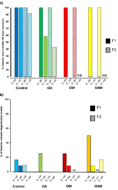
Survival. Under ocean warming (OW) and ocean acidification*warming (OAW) scenarios, O.

317

robusta reached 100 % mortality after 49 and 37 d of exposure respectively (Fig. 1a; Appendix S6, Electronic

318

Supplementary Material). However, mortality was only 33 % under ocean acidification (OA) and significantly

319

higher than that measured under control (C) scenario (χ2 _{= 10.56; P = 0.01). All females of O. japonica}

320

survived the exposure period in all four scenarios (Fig. 1a).

321

Growth rates and degeneration events. Ophryotrocha robusta grew significantly faster (0.17 ± 0.02

322

chaetigers d -1_{) than O. japonica (0.14 ± 0.003 chaetiger d} -1_{) (‘species’ effect, Table 2a), and neither}

323

‘scenario’ in isolation nor its interaction with ‘species’ affected growth rates. Conversely, degeneration events

324

occurred under all scenarios, but showed higher incidence in O. robusta (χ2 _{= 11.28, P = 0.01; Fig. 1b). On}

325

the one hand, 25 % of O. robusta females exposed to OA and OW lost chaetigers, and this percentage

326

doubled under OAW scenario. On the other hand, only 8 % of O. japonica females exposed to OW and OAW

327

showed degeneration events and at a rate comparable to that observed under the C scenario (Fig. 1b).

328

Reproductive success. In O. japonica, 91.67 and 83.33 % of pairs produced viable offspring under

329

OW and OAW, respectively, whilst none of O. robusta pairs reproduced in both scenarios (Fig. 2). Under

330

OA, all O. japonica pairs produced viable offspring, while 75 % of O. robusta pairs did (χ2 _{= 121.97, P <}

331

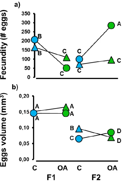
0.001; Fig. 2). Fecundity and egg volume changed in the two species depending to the scenario of exposure,

332

as indicated by the presence of a significant ‘species’*’scenario’ interaction (Table 2a). Ophryotrocha robusta

333

had failed to reproduce under OW and OAW, while O. japonica showed a 10 and 20 % decrease in fecundity

334

and a 35 and 18 % increase in egg volume under OW and OAW, respectively, compared to the C scenario.

335

Under OA, fecundity decreased by 33 and 75 % in O. robusta and O. japonica, respectively (Table 2a; Fig

336

3a), while in both species egg volume did not change when compared to the C scenario (Table 2a; Fig 3b).

337

11

339

Survival. All O. japonica females survived the exposure to C and OA at both generations.

340

Ophryotrocha robusta, on the contrary, showed no mortality events under the C scenario at F1, but it suffered

341

a 9.09 % mortality at F2 (Fig. 1a). Under OA, O. robusta survival was higher for F1 females (58 %) than for

342

F2 females (43 %) (χ2 _{= 9.58; P = 0.01; Fig. 1a).}

343

Growth rates and degeneration events. Ophryotrocha robusta grew significantly faster (0.21 chaetigers d-1₎

344

than O. japonica (0.16 chaetigers d-1_{) (‘species’ effect, Table 2b) and both species had significantly higher}

345

growth rates at F1 (0.24 chaetigers d-1_{) when compared to F2 (0.20 chaetigers d}-1_{), as indicated by the term}

346

‘generation’ being significant (Table 2b). Degeneration events occurred in 8 % of O. robusta females at F1,

347

while they were not recorded at F2 in both species (Fig. 1b).

348

Reproductive success. Under OA, all F2 pairs of O. japonica produced viable offspring, while only

349

58 % of O. robusta pairs reproduced (Fig. 2). However, these differences were not detected as being

350

significant (χ2 _{= 7.59; P = 0.06). In both species, fecundity measured at F1 under OA was lower than in the C}

351

scenario. However, in F2 whilst O. japonica maintained the same fecundity as in F1, O. robusta increased

352

fecundity by 187 % compared to the C scenario, as indicated by the presence of a significant three-way

353

interaction between the terms ‘species’, ‘scenario’ and ‘generation’ (Table 2b; Fig 3a). A significant

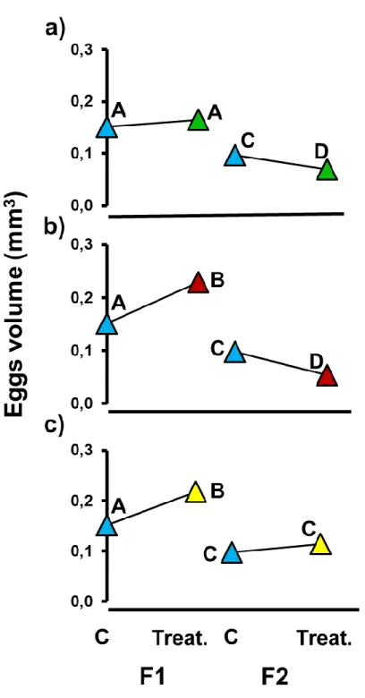
354

interaction between ‘species’, ‘scenario’ and ‘generation’ was also found for egg volume (Table 2b; Fig 3b).

355

While in both species the volume of the eggs laid did not change between scenarios at F1, at F2 it increased

356

under OA in O. robusta to values that were significantly higher than those recorded under the C scenario (+

357

33.33 %). Similarly, but with a reverse trend, egg volume decreased under OA in O. japonica to values that

358

were significantly lower than those recorded under the C scenario (- 30 %) (Fig. 3b).

359

360

Ophryotrocha japonica trans-generational responses (F1-F2) to all ocean global change

361

scenarios

362

Growth rates and degeneration events. Ophryotrocha japonica growth rates were significantly

363

higher at F2 than F1, as indicated by the term ‘generation’ being significant (Tab. 2c), but they did not differ

364

among scenarios (Table 2c). In F2, degeneration events were detected only under OAW in 16.67 % of

365

females (Fig. 1b).

366

Reproductive success. All O. japonica pairs produced viable offspring in both generation and all

367

scenarios tested (Fig. 2). F2 females were significantly more fecund than F1 ones, as indicated by the term

368

‘generation’ being significant (Table 2c), but their eggs were on average smaller than those produced during

369

F1. This trend changed depending on the scenarios, as indicated by the presence of a significant

370

‘scenario*generation’ interaction for egg volume (Table 2c; Fig 4). In more detail, F1 eggs were characterised

371

by a larger volume when exposed to OW and OAW compared to the C scenario, whilst no significant

372

difference was found between OA and C scenarios. This trend changed in F2, where egg volume was

373

negatively affected by the exposure to OA and OW (Fig 4a, b), but it did not change under OAW (Fig 4c).

374

12

Metabolomics profiles comparison

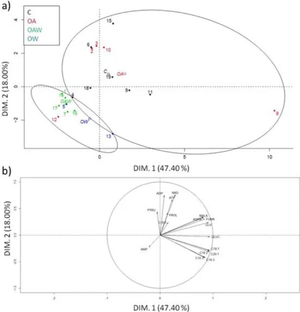
376

Metabolomic profiles were compared among the four scenarios in O. robusta individuals from F1

377

(Fig. 5a). The two axes of the PCA explained 65 % of the total variation, and a significant ‘scenario’ effect

378

was found (F1,10 = 2.90, P = 0.01). The metabolomic profile of individuals exposed to C and OA conditions

379

clustered separately from the scenarios involving elevated temperature (i.e. OW and OAW). The separation of

380

these two groups was mainly driven by a reduction in the concentration of molecules involved in the energy

381

metabolism (Fig. 5b). Specifically [ATP], [ADP], [glutamate], [malate], [fumarate] and [aspartate] were

382

lower under OW and OAW, compared to C and OA conditions.

383

A second PCA documented in O. robusta and O. japonica significant differences in the metabolomic

384

profile after F1 exposure to OW and OAW (F3, 12 = 20.30, P = 4.64 e-05; Fig. 6a). The first axis explained 50.3

385

% of the variation mainly driven by differences in fatty acid composition, while the second axis accounted for

386

21.4 % of the variation, correlated to metabolites involved in the energy metabolism (Fig. 6b). Specifically,

387

the stearic acid C18:0 was more present in O. robusta, while [ATP], [NAD], [glutamate], [glucose] and

388

[aspartate] were in higher concentration in O. japonica.

389

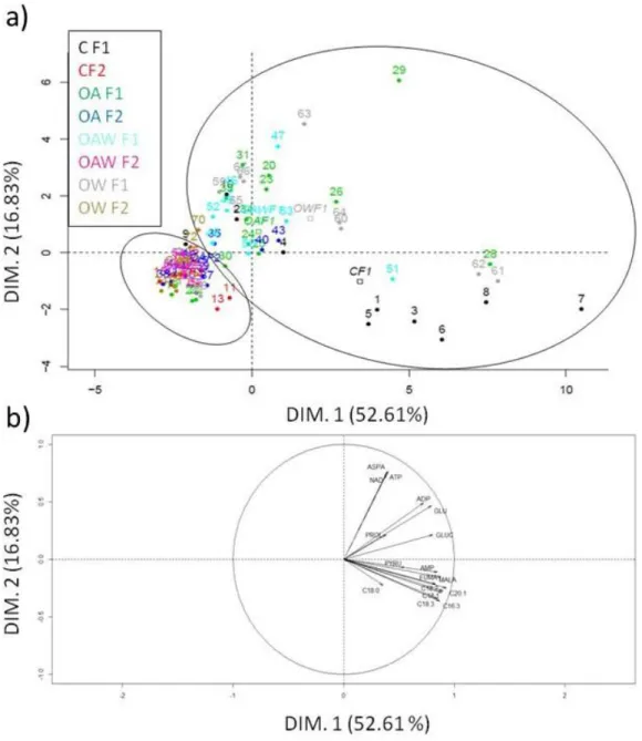
Finally, a third PCA compared the metabolomic profiles from F1 and F2 females of O. japonica (Fig.

390

7). Significant ‘generation’ and ‘scenario’ effects (F3, 32 = 1.76, P = 0.017) differentiated the metabolomic

391

profile of the two generations, with the first two axes explaining 69.44 % of the variation (Fig. 7a). During F1

392

exposure, the metabolite composition in C conditions differed from that in OA, OW and OAW, a distinction

393

driven by differences in fatty acid reserves. In control conditions, females showed higher levels of fatty acid

394

reserve (C16:3, C18:2, C18:1, C20:1, C18:3), [fumarate], [malate] and [AMP] (DM. 1 = 52.61 %).

395

Conversely, no difference between control and global change scenarios was observed for F2. The F2

396

generation differed from F1, as it showed lower concentrations for molecules involved in the cell energy

397

metabolism, i.e. [ATP], [ADP], [NAD], [aspartate], [glutamate] and [glucose] (DIM. 2 = 16.83 %) (Fig. 7b).

398

399

Discussion

400

Our study provides, for the first time, empirical evidence supporting a significant level of divergence

401

in across-generation impacts of combined ocean warming (OW) and ocean acidification (OA) on life-history

402

traits in two congeneric marine species. In addition, we offer a mechanistic underpinning for the observed

403

patterns of sensitivity via metabolomic profiling. We show that the annelid Ophryotrocha robusta is

404

significantly less tolerant to OW and OA, both in isolation and combined (OAW), when compared to its

405

congeneric O. japonica. Overall, chronic exposure to elevated temperature represents the main factor

406

negatively affecting O. robusta fitness, as elevated temperature levels tested are lethal before the species is

407

able to produce a viable progeny. As expected, the combined effect between OW and OA causes a greater

408

negative impact on O. robusta life history performances. Within- and trans-generational responses vary

409

between traits allowing for life-history and physiological adjustments that differ greatly between the two

410

species. Altogether, the common species, O. japonica, thrives across all scenarios, whilst the endemic species,

411

O. robusta, shows tolerance levels well below the magnitude of temperature and pH change expected for the

412

13

413

evidence for whether extant endemic or rare species show greater vulnerability to combined environmental

414

change drivers, our results are consistent with the hypothesis that rare species may be more sensitive to global

415

changes compared to their more widespread congeners (e.g. Bozinovic et al. 2011; Calosi et al. 2008; Calosi

416

et al. 2010).

417

418

The severe effect of ocean warming on O. robusta

419

Future OW and OAW scenarios represent sub-optimal conditions that will be detrimental to the

420

measured functions of O. robusta. Individuals of this species do not survive past 49 d of chronic exposure to

421

OW conditions, despite being already sporadically exposed in the field to the test temperature, and most

422

importantly, they do not produce any viable progeny. In addition, 100 % mortality is reached under OAW

423

conditions within 37 d, indicating the presence of an interactive effect between OW and OA. Growth patterns

424

are also negatively affected, as confirmed by a marked increase in degeneration events. Temperature increases

425

are known to accelerate the metabolic rates up to a maximum level at optimal temperature, beyond which the

426

thermal stability and function of structural proteins and enzymes are compromised. This is followed by

427

physiological failure, by mean of accumulation of thermal-related damages, which sets the upper thermal

428

tolerance limits of marine ectotherms (Hochachka and Somero 2002). The metabolomics profiles of O.

429

robusta under OW and OAW support this idea of a physiological breakdown. Individuals exposed to these

430

scenarios experience in fact a decrease in energy availability, as indicated by the reduction in [ATP], a key

431

metabolite in cellular energetics, and [NAD], a cofactor implicated in the redox reactions of electron

432

transport, together with a decrease in a number of molecules also involved in the Krebs’s cycle, when

433

compared to the profiles of individuals exposed to C and OA scenarios. Under a sustained chronic exposure to

434

warming scenarios, these changes in the energy metabolism could cause the shutdown of O. robusta most

435

sensitive and demanding functions such as reproduction and growth, while gradually leading worms toward a

436

phase of irreversible physiological damage and, ultimately, to death (Pörtner and Gutt 2016). It is important to

437

mention that in our experiment, the physiological impairment we report was accompanied by the cessation of

438

feeding activities, evidenced by the lack of visible food in the worms’ intestines, and the gradual deterioration

439

of the worms’ physical conditions in individuals kept under elevated temperature. This was highlighted by the

440

abnormal increase in the volume of the coelomic cavity of certain individuals. In contrast, all individuals of

441

O. japonica survive and more than 80 % produce viable progeny under OW and OAW. They also lay larger

442

eggs under these conditions, suggesting an increase in parental investment.

443

Differences in metabolomic responses of O. robusta and O. japonica help explain observed trends in

life-444

history traits, as contrary to what was observed for O. robusta, O. japonica increases its energy production in

445

F1 when exposed to global change scenarios: as shown by an increase in [ATP], [NAD] and [aspartate]. This

446

increase is, however, accompanied by a decrease in lipid content. These changes suggest that energy

447

metabolism is likely enhanced in O. japonica, enabling it to maximise important functions at a higher level of

448

biological organisation. The decrease in lipid content we report suggests the existence of potential long-term

449

14

450

Wegner 2014; Gibbin et al. 2017a; Jarrold et al. 2019), and may explain the reduction in egg volume reported

451

for O. japonica after two generations of exposure to the OW scenario. However, in the F2 of O. japonica,

452

lipid content is comparable between C and all global change scenarios, suggesting the capacity of this species

453

to reach a complete metabolic recovery after two generations of exposure. This said, Gibbin et al. (2017a)

454

showed that physiological impairment caused by global change drivers may be detectable in terms of fitness

455

again or only after multiple generations.

456

457

Trans-generational plasticity can help species to cope with global changes, but it is no

458

silver bullet

459

Ocean acidification is the only global change scenario tested in this study where O. robusta produces

460

a viable progeny. However, even under this scenario, this species shows a higher sensitivity compared to O.

461

japonica across both generations. After 49 d of exposure in F1 O. robusta shows 40 % mortality, and around

462

25 and 40 % of surviving females do not reproduce at F1 and F2, respectively. In contrast, no mortality or

463

reproductive failure is detected in O. japonica in both generations.

464

In our study, the two species show similar patterns of trans-generational responses for growth rates to

465

OA, this scenario causing a reduction in growth at F2 when compared to control conditions. It has been

466

widely documented that OA can negatively impact growth through non-beneficial plastic responses, as the

467

increase in energetic requirements needed to maintain homeostasis affects organisms’ ability to maintain and

468

repair their cellular systems (Melzner et al. 2009; Stumpp et al. 2012). The effect of OA on growth rates has

469

been observed within a generation when exposure included early life stages (Chakravarti et al. 2016). This

470

said, evidence also exists for the partial or total restoration of growth performances after two generations of

471

exposure to OA (Parker et al. 2012; Miller et al. 2013; Chakravarti et al. 2016).

472

In O. robusta, the decrease in growth rate following the trans-generational exposure to OA is

473

accompanied by a marked increase in fecundity levels compared to F1 and by an increase in parental

474

investment (Rodriguez-Romero et al. 2016; Bouquet et al. 2018). Even the fecundity of O. japonica benefits

475

from trans-generational exposure to OA, as the reduction in eggs output observed at F1 is fully recovered in

476

the following generation albeit at the expense of egg volume. The re-allocation of the energy among different

477

functions through life-history trade-offs appears to provide the mechanism underpinning the observed

trans-478

generational plastic responses. In O. robusta, trade-offs occurring under OA scenario may account for energy

479

being diverted from growth to reproduction, as documented for other marine species when exposed to

480

increasingly challenging environmental conditions (Pistevos et al. 2011).

481

No trade-offs between life-history traits are detected in O. japonica, this species showing higher

482

tolerance to all global change scenarios tested across both generations when compared to O. robusta. In O.

483

japonica, trans-generational adjustments are observed for survival, growth rates and fecundity, but are not

484

determined by the scenarios tested. Eggs’ volume is the only trait positively affected by acute exposure to

485

OW and OAW, as described previously, but this beneficial plastic response observed in F1 disappears

486

15

487

pattern is accompanied by an energy trade-off between fatty acid reserves and energy production across

488

generations: the former decreasing and the latter increasing under global change scenarios when compared to

489

C conditions. In F2, differences in metabolite concentrations between global changes and C scenarios are no

490

longer evident, suggesting that individuals adjust their metabolism to cope with elevated temperatures and/or

491

pCO2 conditions by the second generation of exposure. Our results differ with those of other studies

492

performed, for example, in marine sticklebacks (e.g. Shama and Wegner 2014; Shama et al. 2014, 2016),

493

juvenile damselfish (Donelson et al. 2012) and even the congeneric annelid Ophryotrocha labronica

494

(Chakravarti et al. 2016). In fact, these studies showed negative effects of high temperature on aerobic

495

metabolism, hatching success or growth rate following acute exposure, after which a complete compensation

496

was observed following trans-generational exposure.

497

Altogether our results confirm that within and trans-gen erational plasticity in both life-history and

498

physiological performances may help some ectothermic species to cope with global change drivers. However,

499

the presence of trade-offs and energy costs associated to plastic responses points to the fact that these

500

mechanisms may not always be beneficial (Shama and Wegner 2014, Chakravarti et al. 2016, Jarrold et al.

501

2019), or be comparable across and among species, as shown in this study by divergent trans-generational

502

effects even between phylogenetically-closely related species. This said, we cannot completely disregard the

503

idea that other mechanisms contributed in determining the trans-generational responses we observed, such as

504

the random sampling of different genotypes across generations or different levels of (long-term) acclimation

505

regimes: F1 being more acute than F2, as F2 individuals complete their entire life cycle under the

506

experimental conditions.

507

In particular, the inability to distinguish between the contribution of selection from that of plasticity in

508

defining trans-generational changes is an intrinsic limitation of global change trans-generational experiments,

509

particularly in sexually reproducing metazoans for which non-breeding designs cannot be easily employed

510

(Gibbin et al. 2017; Donelson et al. 2019). This said, several studies have provided evidences for the

511

occurrence of rapid evolutionary changes across two generations whenever the high selective pressure of the

512

new environment causes a significant increase in mortality levels (> 50 % per generation) (Vidal and Horne

513

2009; Christie et al. 2012; Thor and Dupont 2015), and/or marked variations in reproductive success

514

(Donelson et al. 2012). Accordingly, the high mortality levels and low reproductive success observed in O.

515

robusta under OA in the F1 could have selected for more tolerant genotypes, whose offspring (F2) showed

516

higher fecundity. Conversely, we assume selection to be of marginal importance compared to TGP in O.

517

japonica under OW and OAW, given we report 100 % survival and high reproductive success (> 80 %) in

518

both scenarios in the F1. Therefore, in this species, it is plausible that the changes observed in the F2 are

519

520

521

Conclusions

522

16

523

changes on marine organisms across successive generations. We confirm that both within- and

trans-524

generational plasticity may represent an important mechanism to help species in coping with rapid

525

environmental changes (Ghalambor et al 2007; Calosi et al 2016; Donelson et al. 2018). However, global

526

changes may be happening too quickly for some species to ‘outrun’ them through plastic responses (Quintero

527

and Wiens 2013; Welch et al. 2014), and the magnitude of abiotic changes may overcome species’ sensitivity

528

levels, as reported in our study. Embracing the diversity and complexity of species’ responses to rapid

529

environmental changes is challenging, but it is needed, if we want to reliably predict the impact of global

530

changes. This said, we do not have the time or resources to test all known species, which however represent

531

only a small fraction of existing species, before the negative effects of global changes on extant biodiversity

532

levels are detected at the regional and global scale (Calosi et al. 2016). It is therefore imperative we set out to

533

test broad eco-evolutionary questions using the most appropriate taxa, in order to define general principles

534

with which to guide a critical understanding of marine biodiversity responses to complex global change

535

scenarios. These will be key to guiding adaptive management of natural resources and biodiversity

536

conservation (Calosi et al. 2016). Our results do not allow us to conclude that the eco-evolutionary forces at

537

play define the differences in within and trans-generational responses reported for the two congeneric

538

annelids species with different biogeography investigated here (see Garland and Adolph 1994). Nevertheless,

539

our results, together with evidence from both the paleo and modern records (Calosi et al. 2019), enable us to

540

generate the hypothesis that differences in species’ physiological niches may represent a plausible explanation

541

for the existence of differences in the pattern of sensitivity of phylogenetically closely-related species. We

542

suggest that endemic and rare species may be at greater risk of decline under global changes, when compared

543

to widespread and common species, even when considering their ability for TGP responses. As such, our

544

work has potential important implications for the level and distribution of biodiversity locally and globally in

545

the future ocean, this ultimately determining community compositions and ecosystems’ functioning (Lyons et

546

al. 2005; Mouillot et al. 2013; Violle et al. 2017). The idea that rare species will be more at risk under global

547

change is increasingly supported (Calosi et al. 2008; Mouillot et al. 2013), but requires further testing on a

548

broader phylogenetic scale within the context of global changes (Calosi et al. 2019). Ultimately, our study

549

provides a rational to investigate TGP through combined future global change drivers among species with

550

551

552

553

554

Compliance with Ethical Standards

555

Conflict of interest

556

The authors declare that they have no conflict of interest

.

557

Ethical approval

17

559

organisms for the study have been followed and all necessary approvals have been obtained.

560

Data availability

561

The datasets generated during and/or analysed during the current study are available from the corresponding

562

author upon reasonable request and are available on the PANGAEA data library.

563

564

Acknowledgements

565

We would like to thank Sarah Jacques and Steeven Ouellet for assisting with DIC analyses, and

566

Daniel Small and Nicholas Beaudreau for the attentive linguistic revision of this MS. This work was financed

567

by NSERC Discovery Program grant (RGPIN-2015-06500), Programme Établissement de Nouveaux

568

Chercheurs Universitaires of FRQNT (No.199173), by the Fond Institutionnel de Recherche of the Université

569

du Québec à Rimouski all awarded to PC, and co-funded by the European Union through the Marie

570

Skłodowska-Curie Post-doctoral Fellowship (Proposal Number: 659359) awarded to GMN. FV and PC are

571

members of Québec-Océan FRQNT-funded research excellence networks. We finally thank the three

572

anonymous reviewers for their insightful comments and suggestions.

573

18

References

574

575

Angiletta MJ (2009) Thermal Adaptation: A theoretical and empirical synthesis. Oxford University Press

576

577

Bouquet J-M, Troedsson C, Novac A, Reeve M, Lechtenbörger AK, Massart W, et al. (2018) Increased

578

fitness of a key appendicularian zooplankton species under warmer, acidified seawater conditions. PLoS ONE

579

13(1): e0190625.

580

581

Bozinovic F, Calosi P, Spicer JI (2011) Physiological correlates of geographic range in animals. Annual

582

Review of Ecology, Evolution, and Systematics 42: 155–179

583

584

Caldeira K, and Wickett ME (2003) Anthropogenic carbon and ocean pH. Nature 425: 365

585

586

Calosi P, Bilton DT, Spicer JI (2008) Thermal tolerance, acclimatory capacity and 531 vulnerability to global

587

climate change. Biology Letters 4: 99–102

588

589

Calosi P, Bilton DT, Spicer JI, Votier SC, Atfield A (2010) What determines a species’ geographical range?

590

Thermal biology and latitudinal range size relationships in European diving beetles (Coleoptera: Dytiscidae).

591

Journal of Animal Ecology 79: 194–204

592

593

Calosi P, De Wit P, Thor P, Dupont S (2016) Will life find a way? Evolution of marine species under global

594

change. Evolutionary applications 9: 1035-1042

595

596

Calosi P, Putnam HM, Twitchett RJ, Vermandele F (2019) Marine Metazoan Modern Mass Extinction:

597

Improving Predictions by Integrating Fossil, Modern, and Physiological Data. Annual review of marine

598

science 11: 369–390

599

600

Chakravarti LJ, Jarrold M, Gibbin EM, Christen F, Massamba-N’Siala G, Blier PU, Calosi P (2016) Can

601

trans-generational experiments be used to enhance species resilience to ocean warming and acidification?

602

Evolutionary applications 9: 113–1146

603

604

Chevin LM, Collins S and Lefèvre F (2013) Phenotypic plasticity and evolutionary demographic responses to

605

climate change: taking theory out to the field. Functional Ecology 27: 967–979

606

607

Côté IM, Darling ES and Brown CJ (2016) Interactions among ecosystem stressors and their importance in

608

conservation. Proceedings of the Royal Society B: Biological Sciences 283: 20152592

609

19

611

generation. Proceedings of the National Academy of Sciences of the United States of America 109: 238–

612

242Dickson AG (1990) Standard potential of the (AgCl (s) + ½ H2 (g) = Ag (s) + HCl (aq)) cell and the

613

dissociation constant of bisulfate ion in synthetic sea water from 273.15 to 318.15 K. Journal of Chemical

614

Thermodynamics 215:29–43

615

616

Dickson AG, Sabine CL, Christian JR (2007) Guide to best practices for ocean CO2 measurements. PICES

617

Special Publication 3:1–191

618

619

Dickson AG and Millero FJ (1987) A comparison of the equilibrium constants for the dissociation of carbonic

620

acid in seawater media. Deep Sea Res Part 1 Oceanographic Research Papers 34:1733–1743

621

622

Donelson JM, Munday PL, McCormick MI, Pitcher CR (2012) Rapid transgenerational acclimation of a

623

tropical reef fish to climate change. Nature Climate Change 2: 30–32

624

625

Donelson JM, Wong M, Booth DJ, Munday PL (2016) Transgenerational plasticity of reproduction depends

626

on rate of warming across generations. Evolutionary applications 9: 1072–1081

627

628

Donelson JM, Salinas S, Munday PL and Shama LN (2018) Transgenerational plasticity and climate change

629

experiments: Where do we go from here? Global change biology 24: 13–34

630

631

Donelson JM, Sunday JM, Figueira WF, Gaitan-Espitia JD, Hobday AJ, Johnson CR et al. (2019)

632

Understanding interactions between plasticity, adaptation and range shifts in response to marine

633

environmental change. Philosophical Transaction of the Royal Society B 374: 20180186

634

635

Duncan EJ, Gluckman PD, Dearden PK (2014) Epigenetics, plasticity, and evolution: How do we link

636

epigenetic change to phenotype? Journal of Experimental Zoology Part B: Molecular and Developmental

637

Evolution 322: 208–220

638

639

Eirin-Lopez J and Putnam M (2019) Marine environmental epigenetics. Annual Review of Marine Science 11:

640

335–368

641

642

Fox RJ, Donelson JM, Schunter C, Ravasi T, Gaitan-Espitia JD (2019) Beyond buying time: the role of

643

plasticity in phenotypic adaptation to rapid environmental change. Philosophical Transactions of the Royal

644

Society B 374: 20180174

645

646

Garland Jr T and Adolph SC (1994) Why not to do two-species comparative studies: limitations on inferring

647

adaptation. Physiological Zoology 67: 797-828

648

20

650

plasticity potentiates rapid adaptive evolution of gene expression in nature. Nature 525: 372

651

652

Ghalambor CK, McKay J, Carroll S and Reznick D (2007) Adaptive versus non-adaptive phenotypic

653

plasticity and the potential for contemporary adaptation in new environments. Functional Ecology 21: 394–

654

407

655

656

Gibbin EM, Massamba N’Siala G, Chakravarti LJ, Jarrold MD, Calosi P (2017a) The evolution of phenotypic

657

plasticity under global change. Scientific Reports 7: 17253

658

659

Gibbin EM, Chakravarti LJ, Jarrold MD, Christen F, Turpin V, Massamba N’Siala G, Blier PU, Calosi P

660

(2017b) Can multi-generational exposure to ocean warming and acidification lead to the adaptation of

life-661

history and physiology in a marine metazoan? Journal of Experimental Biology 220: 551–563

662

663

Gibson R, Atkinson R, Gordon J, Smith I, Hughes D (2012) Impact of ocean warming and ocean acidification

664

on marine invertebrate life history stages: vulnerabilities and potential for persistence in a changing ocean.

665

Oceanogr Mar Biol Annu Rev Annual Review 49: 1–42

666

667

Griffith AW, Gobler CJ (2017) Transgenerational exposure of North Atlantic bivalves to ocean acidification

668

renders offspring more vulnerable to low pH and additional stressors. Scientific reports 7: 11394

669

670

Hall POJ, Aller RC (1992) Rapid, Small-Volume, Flow Injection Analysis for ΣCO2 and NH4+ in Marine and

671

Freshwaters. Limnology and Oceanography 37:1113–1119

672

673

Hofmann GE (2017) Ecological epigenetics in marine metazoans. Frontiers in Marine Science 4: 4

674

675

Hoshijima U, Hofmann GE (2019) Variability of seawater chemistry in a kelp forest environment is linked to

676

in situ transgenerational effects in the purple sea urchin, Strongylocentrotus purpuratus. Frontiers in Marine

677

Science 6: 62

678

679

Husson F, Lê S, Pagès J (2017) Exploratory multivariate analysis by example using R. Chapman and Hall

680

681

Hutchinson GE (1978) An Introduction to Population Ecology. Yale University Press

682

683

IPCC (2014) Climate Change 2014: The physical science basis: contribution of working group I to the fifth

684

assessment report of the Intergovernmental Panel on Climate Change. New York, USA: Cambridge

685

University Press

686