LES of combustor-turbine
interactions
Indirect combustion noise generation
in a high-pressure turbine
Contents
5.1 Motivation . . . 92
5.2 Indirect combustion noise state-of-the-art . . . 93
5.3 DMD test case: 2D entropy spot propagation in a periodic channel . . 95
5.4 Turbine stage simulation set-up . . . 99
5.4.1 Mesh . . . 100
5.4.2 Numerical schemes . . . 100
5.4.3 Boundary Conditions . . . 101
5.5 Numerical Results . . . 105
5.5.1 Overall flow topology . . . 105
5.5.2 Dynamic Mode Decomposition of the LES flow field . . . 107
5.5.3 Quantifying the indirect noise and comparisons with the com-pact theory . . . 117
5.6 Conclusions . . . 119
This chapter details the first application of the MISCOG method to combustion cham-ber/turbine interactions: the indirect combustion noise generated across a high-pressure turbine from temperature non-uniformities. As with most previous investigations of this process, a decoupled simulation of a turbine stage from the combustion chamber is per-formed. The consequence of this choice is that the temperature non-uniformities do not come from the unsteady combustion process. Instead, they are modeled by sinusoidal fluctuations introduced by boundary conditions in the turbine stage alone. The acoustic response of the turbine is then analyzed with a specific interest on the indirect noise generation mechanisms. A part of this work was performed during the author’s partici-pation to the Summer Program of the Center for Turbulence Research (CTR) at Stanford
University. Results have been published in the proceedings of the summer program [177], the ASME Turbo Expo 2015 conference [178] and will also appear in the Journal of Turbomachinery.
5.1
Motivation
According to the International Civil Aviation Organization (ICAO), the world passenger traffic has increased on average by 5.8% per year throughout this decade and the European Union predicts that without any substantial technological improvements, the number of people in Europe that will be a↵ected by high levels of aircraft noise will double by the year 2026 [179]. Consequently, ACARE’s Vision 2050 calls for increased research in the field to reduce the perceived noise by 65% until 2050, with respect to a new aircraft built in 2000. Engines are the main noise source in commercial and military aircraft. For helicopters, the main noise source is still and will remain for some time the rotor blades of the vehicle, hence reducing the significance of the gas turbine noise. Nonetheless, recent studies (for example in the frame of the TEENI project) clearly indicate traces of engine noise emitted from such aircraft.
The first studies on gas turbine noise, carried out by Lighthill [180], showed the importance of jet noise on the overall noise emitted by an aircraft. Lighthill showed that jet-noise scaled with the eighth power of the jet-exhaust speed, meaning that doubling the jet speed would lead to an increase of the acoustic intensity level by nearly 50 dB. The development of the turbofan engine alleviated significantly this issue thanks to the fact that the majority of the propulsion comes from a cold by-pass flow stream, with large mass flow and low speed, resulting in a drastically reduced jet noise. Jet noise has been reduced to the point that the noise emitted from the other components, notably from the fan, the compressors/turbines and the combustion chamber, is becoming more important. Figure 5.1 compares the noise contributions of the di↵erent gas turbine components and the noise directivity from an early turbojet engine and a modern turbofan engine. It is evident that in the latest designs fan noise is the prevalent source. However, as further reductions on fan noise are achieved, the relative importance of combustion noise, also called core noise, whose contribution stayed unchanged over the years, is increasing. This suggests that further research on combustion noise is essential if a continuous reduction of the overall engine noise levels is envisioned for the next years. This has led to a renewed interest in the topic with several dedicated EU projects forming the last five years, such as TEENI1 and RECORD2.
Combustion noise is principally a low-frequency noise generated in the combustion chamber of gas turbines and arising from two main mechanisms, as mentioned in Chapter 1. First, direct noise emanates from the acoustic waves created at the unsteady flame front and propagated through the rest of the engine. It is a source of noise that has received considerable attention in the past [181, 182, 183, 184]. Second, the unsteady combustion will give rise to low-frequency temperature fluctuations, or entropy waves,
1Turboshaft Engine Exhaust Noise Identification
Figure 5.1: Noise emissions and directivity of gas turbine components - Typical 1960’s turbojet engine (left) and a recent 1990’s turbofan design (right) [17].
that are convected with the flow velocity to the combustor nozzle and turbine. There, the waves are subject to significant acceleration and distortion in the blade passages, generating acoustic waves in the process. This noise generation mechanism is called indirect and its importance is twofold: (a) it increases the noise signature of the engine and (b) the acoustic waves propagating upstream can impact the thermoacoustic stability of the combustion chamber [1, 35]. Leyko et al. [18] computed analytically the ratio between indirect and direct combustion noise for di↵erent operating conditions, modeling the flame in the combustor and the nozzle at the combustor exit as jump conditions. The results, Fig. 5.2, indicate that for the typical operating conditions of aeronautical gas turbines (red point), indirect combustion noise will likely be the dominant source of combustion noise. Yet its actual relevance remains controversial.
5.2
Indirect combustion noise state-of-the-art
Due to the complexity of a full 3D HPT, past theoretical and numerical studies have used simplified turbine-like geometries. The first in-depth analyses on turbine-like geometries focused on the propagation of entropy waves through quasi-1D nozzles. In this context, Marble and Candel [37] developed an analytical method to evaluate the transmission co-efficients of acoustic and entropy waves propagating through a compact quasi-1D nozzle, its length being significantly smaller than the wavelength of the incoming waves. More recently, Duran and Moreau [34] proposed an analytical method to calculate the trans-mission coefficients of general quasi-1D nozzles, removing the compact nozzle assumption. These analytical methods, accompanied by numerical predictions from LES, have been evaluated on the experimental Entropy Wave Generator [40], with [18] and [42] reporting
Figure 5.2: Estimation of the ratio ⌘ between indirect and direct noise by an analytic ap-proach. The ratio ⌘ is plotted here as a function of the Mach number M1 representing the Mach number in the combustion chamber and at the nozzle inlet, and of the Mach number M2 representing the outlet nozzle Mach number - Typical combustor operating point indicated with a red point [18].
good agreement on both subsonic and supersonic operating conditions. The same prob-lem was also treated theoretically by Howe [36], who used the compact hypothesis with an acoustic analogy and highlighted the impact of the entropy wave form on the gener-ated noise. A potential coupling of indirect combustion with vortex noise from separgener-ated flow regions at the nozzle walls was revealed to be an influencing factor on the measured noise.
The theory of Marble and Candel for nozzles was extended to 2D compact blade rows by Cumpsty and Marble [38], taking into account the reorientation of the flow. This is achieved by imposing an additional constraint, the Kutta condition at the blade trailing edge. The method was originally conceived for a single blade row and tested against numerical simulations by several authors, both for compact and non-compact frequencies [185, 186]. It was extended to multi-stage turbines by Duran et al [187] and was compared against numerical simulations of a 2D high-pressure turbine stage as well as experimental results of [39] for a 3-stage turbine (NASA test case 1629).
The present work is the first numerical evaluation of the indirect combustion noise generated in a realistic, fully 3D, transonic high-pressure turbine. As it was observed in the previous chapters, the flow across a realistic turbine is much more complex than in 2D simulations, where no endwall e↵ects are present and turbulence evolves di↵erently. The operating point of these 2D studies was also subsonic [34, 185], instead of the typical transonic conditions encountered in real configurations. As a result, the mixing of the entropy waves as they go through the turbine and the indirect noise generation is expected to be altered. This simulation can, thus, serve as an additional validation of previous
simulations as well as to calibrate lower order models, such as the one developed in [18]. To do so, a train of sinusoidal entropy waves of constant frequency and amplitude is injected in the MT1 high-pressure turbine, detailed in Chapter 4, to model the entropy waves generated in a combustor (details on the entropy wave injections are provided in section 5.4.3). While combustion noise is broadband in nature, a monochromatic pulse allows to easily distinguish it from other turbine noise sources. Note that for this study, the Dynamic Mode Decomposition (DMD) is employed and deemed necessary for an adequate analysis of the predicted flow field [188].
Analyzing high-fidelity numerical simulations of flows characterized by complex, dy-namic and non-linear systems can be particularly cumbersome. Such systems might be exceedingly hard to analyze directly by simple visualization or statistical techniques (ei-ther due to excessive memory demands or convergence issues). Advanced methods have emerged during the last decades to provide a detailed analysis of many flow fields. Dy-namic Mode Decomposition is one of the most recent methods to appear [188] and it attempts to identify coherent single-frequency structures from a series of flow snapshots. The DMD has been selected here compared with other frequency-domain methods, for its robustness and the resolution capabilities with only few periods per frequency of interest included in the signal. Additionally, the method minimizes spectral leakage. It also pro-vides both global information, in the form of spectra as well as the spatial structure of the computed modes.
In the following section, the method is validated on a simple 2D test case, illustrat-ing the information that DMD provides and investigatillustrat-ing its potential advantages and limitations. At the same time, the test case allows to validate the entropy wave injection through the boundary conditions. A description of the derivation of DMD is provided in Appendix C. The forced turbine simulations are presented in section 5.4 while section 5.5 discusses the results from the numerical simulations and quantifies the generated indirect combustion noise.
5.3
DMD test case: 2D entropy spot propagation in
a periodic channel
To illustrate the DMD capabilities, a simple test case is employed: the propagation of an entropy wave across a 2D, periodic in the transverse coordinate, channel. To remove any di↵usion e↵ects, the Euler equations are resolved. The inflow consists of a uniform axial velocity U = 10 m/s at ambient conditions, i.e T = 300 K and P = 1.01298 bar respectively. At the inlet a sinusoidal entropy wave of frequency f = 4 kHz and ampli-tude T p = 20 K is also introduced through the characteristic boundary conditions2. A schematic of the test case with the boundary conditions employed is presented in Fig. 5.3. For demonstration and validation purposes, DMD is also compared with the Fast Fourier Transform (FFT) of the signal recorded at a probe placed at the center of the channel.
2A description on the introduction of waves through the characteristic boundary conditions is
L = 0.01 m h = 0.001 m Inlet U=10m/s Tmean = 300K Tp= 20K f = 4kHz Outlet Periodic B.C Probe for FFT Periodic B.C
Figure 5.3: Schematic of the 2D test case and boundary conditions employed.
Figure 5.4: Instantaneous temperature flow field of the 2D test case.
The simulation run for four periods of the wave frequency and the sampling frequency for the flow field snapshots is 10 kHz. The sampling frequency at the temporal probe is the same as for the DMD and is chosen to be superior to the Nyquist frequency. Figure 5.4 depicts the temperature of the flow field obtained from an instantaneous solution. The form of the injected sinusoidal entropy wave with amplitude 20 K is evident. The entropy pulsation is convected by the flow and its wavelength can be easily computed: = Uf = 0.0025 m.
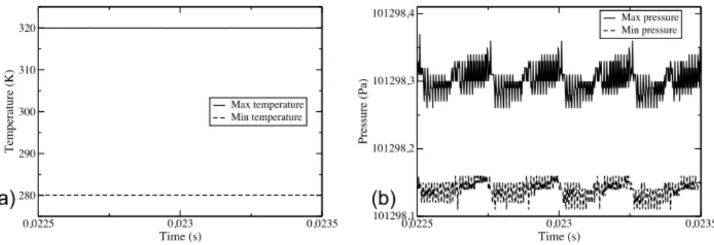
The maximum and minimum temperature in the domain, as a function of time, are presented in Fig. 5.5(a). The recovered values correspond perfectly to T ± T p, high-lighting that the entropy waves are injected correctly and no additional perturbations on the temperature are generated. An important requirement is that the forcing does not generate acoustic waves. If acoustic waves are generated by the boundary conditions they can pollute the indirect noise measurements. To verify that, the maximum and minimum pressure of the domain are also investigated, Fig. 5.5(b), and indicate that the di↵erence between the two is less than 0.2P a, confirming that the entropy forcing is, indeed, ”quiet”.
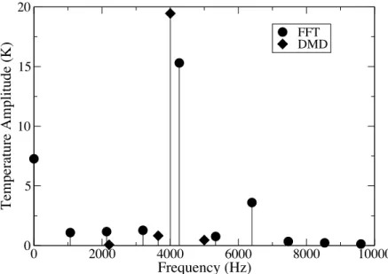
Figure 5.6 depicts the temperature spectrum from the DMD analysis of the flow field snapshots along with the FFT of the temperature signal recorded at the temporal probe. It is evident that DMD captures correctly the introduced wave both in terms of frequency (4 kHz) and amplitude (20 K) with no other significant mode appearing. Note that comparatively and for this set of sampling frequency and signal duration the FFT is incapable to capture correctly neither the amplitude nor the frequency. Improving the frequency prediction would require increasing the FFT length to a size that divides
0,0225 0,023 0,0235 Time (s) 101298,1 101298,2 101298,3 101298,4 Pressure (Pa) Max pressure Min pressure 0,0225 0,023 0,0235 Time (s) 280 290 300 310 320 Temperature (K) Max temperature Min temperature (a) (b)
Figure 5.5: Maximum and minimum temperature (a) and pressure (b) across the domain as a function of time. Entropy forcing of amplitude 20 K is active.
the frequency of interest closer to an integer or use of the zeropadding technique in the signal. Improving the amplitude can only be obtained by simulating longer periods of the phenomenon. These difficulties typical of FFT analysis confirm that DMD can provide reliable information with a considerably reduced number of snapshots and without additional treatments.
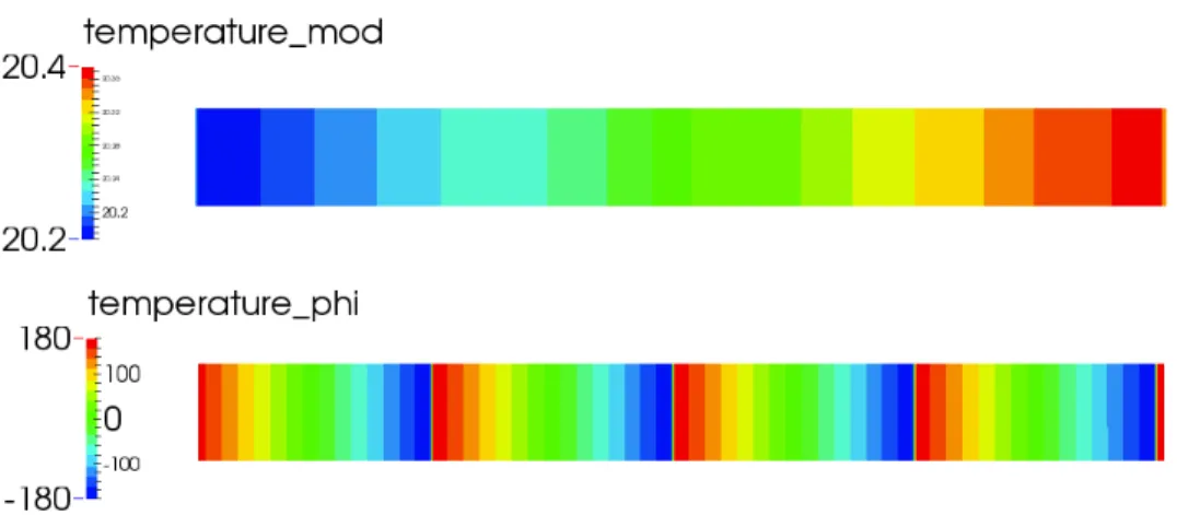
To confirm further that DMD captures accurately the introduced waves, the spatial form of the 4 kHz mode, in terms of temperature modulus and phase across the domain, is presented in Fig. 5.7. The depicted temperature modulus (top) is, indeed, showing the right entropy wave amplitude with minimal variation across the domain, despite the fact that only 4 periods T of the phenomenon were e↵ectively computed. The phase of the temperature, Fig. 5.7(bottom), provides information on the propagative direction of the waves. As it changes linearly across the axial direction and there is no variation across the transverse coordinate, purely axial propagating entropy waves are observed, as anticipated for this simple test case.
From these results, it is evident that DMD can provide a wide range of information, both global and local, at an a↵ordable cost and high precision. To investigate further the limits of DMD, a parametric analysis of the temperature spectra is performed in the following: a) for a varying sampling frequency and a total runtime of 4 periods and b) for a varying runtime and a constant sampling frequency of 10 kHz.
E↵ect of sampling frequency
The first step is to evaluate the impact of the sampling frequency. A method capable of finding the oscillatory motions with low sampling frequencies is particularly advantageous: the memory requirements for storing the necessary information indeed would reduce drastically and the CPU cost decreases if the code does not need to pass through the routines that create solution files. These aspects are particularly important in large LES where storage requirements of a single solution file can be of the order of Gigabytes.
In this simple test case there are no other oscillatory phenomena present apart from the entropy forcing so the e↵ect of the sampling frequency can be straightforwardly evaluated. The sampling frequency can be reduced up to the Nyquist frequency, that is twice the
0 2000 4000 6000 8000 10000 Frequency (Hz) 0 5 10 15 20 Temperature Amplitude (K) FFT DMD
Figure 5.6: DMD temperature spectrum of the 2D test case and FFT of the temperature signal captured at a probe in the center of the channel.
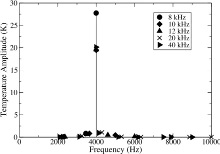
frequency of the phenomenon of interest. Higher sampling frequencies are also tested. The temperature spectra for sampling frequencies ranging from 8 40 kHz are presented in Fig. 5.8. The total runtime remains 4 periods of the entropy wave frequency. It is evident that even with the minimum possible sampling frequency of 8 kHz the pulsating mode is recovered, albeit with an overpredicted amplitude. For sampling frequencies of 10 kHz and higher the amplitude prediction improves considerably and the results reach the desired 20 K amplitude.
E↵ect of runtime
Another important parameter, apart from the sampling time, is the runtime during which the flow snapshots are recorded. It is desirable for any frequency domain method to be reliable after few periods of the oscillating phenomenon of interest have been simulated by the CFD solver. This limits the computational cost and facilitates the post-processing since again less memory is required to save and process the data. As was observed in Fig. 5.6, FFT has difficulties in recovering oscillatory phenomena with as few as 4 periods. Figure 5.9 depicts the DMD temperature spectra for di↵erent runtimes (hence di↵erent total number of snapshots) and constant sampling frequency of 4 kHz. It is evident that DMD recovers the mode with only 2 periods and with approximately the correct amplitude. A slight improvement on the amplitude prediction is the only outcome of the runtime increases. These findings highlight the potential of the method on more realistic flow configurations.
These findings suggest that DMD is a very reliable and robust method. However, as the proposed test case is very simple and lacks any stochastic fluctuations, a convergence
Figure 5.7: DMD 4 kHz mode - Temperature modulus (top) and phase (bottom).
study with respect to di↵erent runtimes is undertaken and detailed later for the turbine stage configuration. This will provide further insight on the method’s capacities in very complex geometries and high Reynolds number flows.
5.4
Turbine stage simulation set-up
The objective of this chapter is to investigate the generation of indirect combustion noise across a fully 3D turbine stage. To this end, the transonic MT1 turbine stage [2] is chosen for this study as it provides a validated and realistic geometry of a high-pressure turbine. As in chapter 4 the scaled geometry is employed with 1 stator blade and 2 rotors (12 degree periodicity) to reduce the computational domain. Two simulations were performed: a) one with a steady inflow that serves as a reference case and b) one where an entropy wave train is introduced at the inlet to evaluate the indirect combustion noise generation process.
In the following, the principal flow characteristics are first identified for both the steady inflow and the forced cases. The analysis of the steady inflow reference simulation using DMD is performed and the most important natural modes are identified. The DMD global spectra of the forced case are then investigated against those of the steady inflow case to evaluate the impact of the incoming entropy waves on the noise generation of the turbine. Afterwards, the response of the flow field at the pulsation frequency for the forced case is examined in further detail on the basis of DMD and transmission coefficients are obtained for the generated acoustic waves. To finish, the results are compared to those obtained with the 2D theoretical model of [38] and 2D pseudo-LES of a similar turbine configuration [189].
0 2000 4000 6000 8000 10000 Frequency (Hz) 0 5 10 15 20 25 30 Temperature Amplitude (K) 8 kHz 10 kHz 12 kHz 20 kHz 40 kHz
Figure 5.8: DMD temperature spectrum of the 2D test case for di↵erent sampling frequencies. Duration of the signal 4T.
5.4.1
Mesh
The mesh employed is, as for the previous MT1 simulations, a fully 3D hybrid mesh with 10 prism layers around the blades and tetrahedral elements in the passage and endwalls. Three views of the mesh are provided in Fig. 5.10. It is composed of 8.1 million cells in total for the stator domain and 10.5 million cells for the rotor domain. It is more refined than the coarse mesh used in Chapter 4 to improve the acoustic predictions and is designed to place the first nodes around the blade walls deeper in the logarithmic region. Note also that a low aspect ratio for the prisms, set to x+ ⇡ 5 y+ ⇡ 5 z+, is maintained to permit a good resolution of streamwise/spanwise flow structures. In the rotor tip region, there are approximately 15 cell layers, as shown in Fig. 5.10(c), in an e↵ort to keep the time step reasonable. In wall units, the maximum values of y+ measured around the blade is approximately 50.
5.4.2
Numerical schemes
As in the previous chapters, the AVBP solver with the MISCOG method is used to perform LES of the MT1 turbine stage. The numerical integration in this chapter is handled by the two-step, finite-element TTGC [119] scheme that is 3rd order accurate in time and space and explicit in time. It is chosen over the cheaper LW scheme for its performance in handling acoustics, an important parameter in this problem. This scheme is used in conjunction with the Hermite-type 3rd order interpolation for the data exchange at the overlap zone, ensuring low dissipation and low dispersion of the rotor/stator interactions, while preserving the global order of accuracy of the numerical
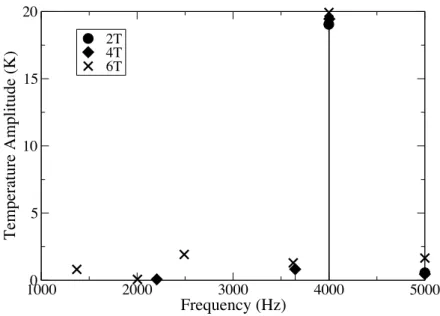
1000 2000 3000 4000 5000 Frequency (Hz) 0 5 10 15 20 Temperature Amplitude (K) 2T 4T 6T
Figure 5.9: DMD temperature spectrum of the 2D test case for di↵erent runtimes. Sampling frequency 10 kHz.
Boundary Euler Navier-Stokes
Subsonic Inflow 4 5
Subsonic outflow 1 4
Table 5.1: Number of conditions required for a well-posed 3D simulation [25].
scheme. The computational cost for simulating the time corresponding to one 360-degree revolution of the turbine stage is 30K CPU hours.
5.4.3
Boundary Conditions
Performing numerical simulations requires from the user to specify certain boundary conditions at the domain limits. Table 5.1 presents the number of necessary conditions to ensure a well-posed problem near the boundaries [25]. In the LES context particular attention on the boundary conditions is required as the compressible LES formalism allows the resolution of acoustic waves generated by the flow, which will propagate and reach the boundaries of the domain. Imposing the necessary boundary conditions in a hard way will lead to the waves being reflected back into the domain thus modifying and polluting the flow field. As a result, treating these waves is necessary to ensure minimal reflection while respecting the user imposed flow parameters.
In AVBP, the boundary conditions follow the NSCBC formulation [118]. In this method, the flow is decomposed into characteristic waves crossing the boundaries using the Linear One-Dimensionsal Inviscid (LODI) relations. Figure 5.11 depicts the charac-teristic waves crossing an inlet and an outlet. Two acoustic waves (upstream propagating
(b)
(c)
(a)
Figure 5.10: mesh view of the stator at mid-span (a) of the rotor at mid-span (b) and at the rotor tip (c)
w and downstream propagating w+) are identified and are complemented by an entropy wave ws and two waves related to transverse variations of the velocity. At the inlet, four of these waves are entering the domain so 4 physical conditions need to be specified. At the outlet one condition is sufficient as only the wave w is entering the domain at this position.
Outlet
At the outlet of the domain, Fig. 5.11 demonstrates that there is only one acoustic wave (w ) coming in the domain that needs to be treated. With the NSCBC method, for the acoustic wave entering the domain from the outlet, w , one writes:
@w
@t L = 0. (5.1)
where L is the amplitude variation of the characteristic wave w that would enter the computational domain. For a perfectly non-reflecting boundary condition L = 0. In practice however this is not possible. In most commonly used outlet conditions, the user wants to impose a static pressure. To recover this desired property while being acoustically nearly non-reflection, a partially non-reflecting formulation is usually used:
L = Kp
p pref pref
INLET OUTLET
w
+w
w
sw
t1w
t2w
+w
w
sw
t1w
t2Figure 5.11: Characteristic waves crossing an inlet and outlet
In Eq. (5.2) Kp is the relaxation coefficient and pref the reference pressure imposed by the user. With this formulation, small values of the relaxation coefficient result in a less reflecting outlet, while large values ensure that the pressure is close to the user-defined target but wave reflection is stronger [190]. For real flow problems where locally 1D flow does not apply, a modification of the NSCBC, described by Granet et al. [191] can also be used, to ensure that vortices created by the blade wakes are leaving the domain without generating noise.
Inlet
At the inlet, the boundary is treated in a similar way. The user-specified physical condi-tions in the investigated case include the total pressure and the total temperature. The incoming acoustic wave (since now it is an inlet) will be a function of these 2 variables. The formula for the incoming acoustic wave reads:
@w+
@t L
+ = 0. (5.3)
with the amplitude of the incoming acoustic wave written as [192] (transverse fluctu-ations are ignored):
L+ = ec K+ Ktt(T t T tref) T ⇢K+ Kpt(P t P tref). (5.4)
where ec is the kinetic energy, P t and T t are the total pressure and temperature, Kpt is the relaxation coefficient on the total pressure, while K+ = (c+u2n)T t + e2ccT, un being the velocity normal to the boundary and c the speed of sound.
Rotational Speed (rpm) 9500 Inlet total pressure (Pa) 4.56e5 Inlet total temperature (K) 444
Mass flow (kg/sec) 17.4
Outlet static pressure (Pa) 1.4· 105
Wave amplitude (K) 20
Wave frequency (Hz) 2000
Table 5.2: Operating conditions of the MT1 turbine.
Note that no turbulent fluctuations are added at the inlet, as only pure indirect combustion noise generated in the turbine is investigated. For the forced simulations, si-nusoidal entropy spots are introduced through the corresponding characteristic equation:
@ws
@t L
s = 0. (5.5)
where ws is the entropy wave. In an unforced simulation, Ls = ⇢(c+un)
2CpT L
++ ⇢
TKtt(T t T tref), with Ktt being the relaxation coefficient of the total temperature. For the forced simulations, one should instead write:
Ls = ⇢(c + un) 2CpT L++ ⇢ TKtt(T t T tref T t s f) + @wfs @t . (5.6) where ws
f = Asin(!t) is the entropy temporal signal of amplitude A and frequency ! injected in the domain and T ts
f is the fluctuation of the total temperature due to this wave.
For the forced LES, the frequency of the imposed waves is fixed at 2 kHz and the amplitude is 4.8% of the inlet total temperature. This value has been shown to gen-erate acoustic waves of linear dynamics [185]. The reduced frequency of the forcing is ⌦ = f Ln/c0 = 0.1, with Ln being the rotor chord length, f the forcing frequency and c0 the speed of sound at the turbine inlet. While combustion noise is usually associ-ated to lower frequencies, 2 kHz was found to be approximately the limit of validity of the compact theory in 2D configurations [189] and renders the simulations more a↵ord-able. Additionally, due to the complexity of this high Reynolds transonic 3D turbine, a monochromatic pulsation is preferred over a more realistic broadband pulsation in an e↵ort to distinguish pure indirect noise from other sources of noise more easily. Note that no acoustic waves are introduced into the computational domain by this approach, as was shown in section 5.3. The operating and boundary conditions employed in this work are summarized in Table 5.2.
0 0.2 0.4 0.6 0.8 1 x/C 0 0.5 1 Mis 0 0.2 0.4 0.6 0.8 1 x/C 1e+05 1.5e+05 2e+05 2.5e+05 3e+05 Pressure Pre ssu re (Pa )! Mi s! x/C! x/C!
(a)
(b)
Figure 5.12: Time-averaged mid-span profiles of the isentropic Mach number across the stator blade (a) and of the static pressure across the rotor blades (b).
5.5
Numerical Results
5.5.1
Overall flow topology
The overall flow topology is analyzed for the two cases. First and in an attempt to validate the mean flow predictions with this mesh (of an intermediate resolution compared to MESH1 and MESH2 of Chapter 4), the isentropic Mach number and the static pressure across the stator and rotor blades are respectively shown on Fig. 5.12(a) and 5.12(b) at mid span for the steady inflow case. The agreement with the experimental measurements is fair and the plots correspond well with the results obtained in the previous chapters for this configuration.
Looking at the full 3D field, as before, a particularly complex flow field is revealed. Figure 5.13 depicts density gradient contours (in logarithmic scales) of the flow across a cylindrical cut at mid-span of the turbine for the steady inflow and pulsed cases, Figs. 5.13(a) and 5.13(b) respectively, complemented by a view in an x-normal plane near the rotor trailing edge for the steady inflow case, Fig 5.13(c). Some of the phenomena highlighted in Fig. 5.13 are the shock/boundary layer interaction on the suction side of both the stator and the rotor (positions A and B), vortex shedding from the trailing edge of the blades and the accompanying acoustic waves emitted (position C), as well as strong secondary flows developing at the endwalls (positions D and E), as observed in Chapter 4. For the pulsed case, Fig. 5.13(b), in addition to the previously highlighted phenomena, the planar entropy waves approaching the stator are also evidenced (position F). As these waves go through the stator passages they get distorted and partially mixed by the blade wakes before being cut by the passing rotors. The mixing and the developing turbulence clearly make the entropy waves less visible in the rotor domain.
Strong 3D secondary flows are highlighted by Q-criterion isosurfaces for an instan-taneous solution of the unpulsed case, Fig. 5.14. It can be observed that on the stator suction side streaky structures are developing as the trailing edge is approached, which result in a flow boundary layer laminar-to-turbulent transition at the trailing edge and a
A
B
C
D
E
F
(a)
(b)
(c)
A
B
C
Figure 5.13: Contours |r⇢|⇢ of an instantaneous solution at mid-span for the steady inflow (a) and pulsed cases (b). Contours of the same variable and at an x-normal plane near the rotor exit for the steady inflow case (c).
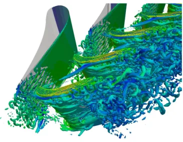
Figure 5.14: Q-criterion of an instantaneous solution across the turbine stage.
fully turbulent vortex shedding. These streaky structures di↵er from the low-resolution simulations of Chapter 4, Fig. 4.15, highlighting the e↵ect of the mesh refinement on the near-wall predictions. Significant activity is also present at the rotor tip, where the tip leakage vortex dominates other unsteady activities.
5.5.2
Dynamic Mode Decomposition of the LES flow field
A frequency domain analysis is performed by applying DMD to a set of instantaneous flow fields to identify the most important noise-generating modes and their origins. It can also be e↵ectively used to investigate both qualitatively and quantitatively the generated combustion noise.
To obtain converged and accurate statistics for the flow, especially in the highly turbulent rotor-blade wake, both the steady inflow and the pulsed simulations ran for a total of 10 periods of the pulsation frequency. As will be shown later in this section, the presence of turbulence necessitates this increase in runtime, in contrast to the findings in the simple 2D test case. To avoid aliasing, the sampling frequency needs to be high enough to include all the important high-frequency phenomena. In this case the vortex shedding from the stator trailing edge is the most significant and resolving it, as well as its first harmonic, is necessary. The necessary sampling frequency was determined to be 120 kHz using a simple FFT of a temporal signal recorded at a probe in the stator wake. Lower sampling frequencies were attempted (60 kHz and 30 kHz) but aliasing errors were present. Since DMD is memory consuming, the decomposition is performed at cylindrical blade-to-blade planes at mid-span with the signal including the six principal primitive variables: pressure, temperature, the three velocity components and density. For the pulsed case, a set of x-normal planes at the inlet and outlet of the turbine stage is also employed to measure the incoming/outgoing acoustic and entropy waves as well as the
0 10000 20000 30000 40000 50000 60000 frequency (Hz) 0.01 0.1 1 10 Temperature amplitude (K) 0 10000 20000 30000 40000 50000 60000 frequency (Hz) 0.1 1 10 Temperature amplitude (K) BPF 6BPF 2BPF BPF 2BPF 12BPF
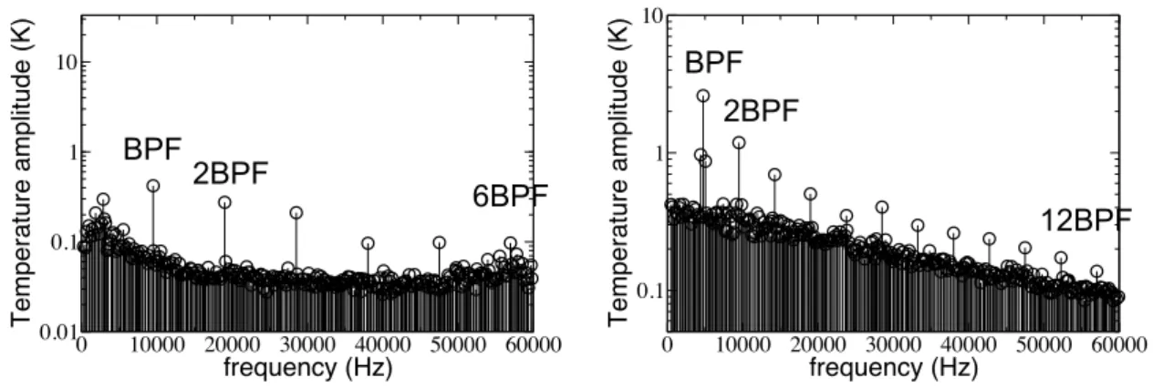
Figure 5.15: DMD temperature spectrums of the stator (left) and rotor domain (right) at mid-span - Steady inflow case.
associated transmission and reflection coefficients. DMD of the steady inflow case
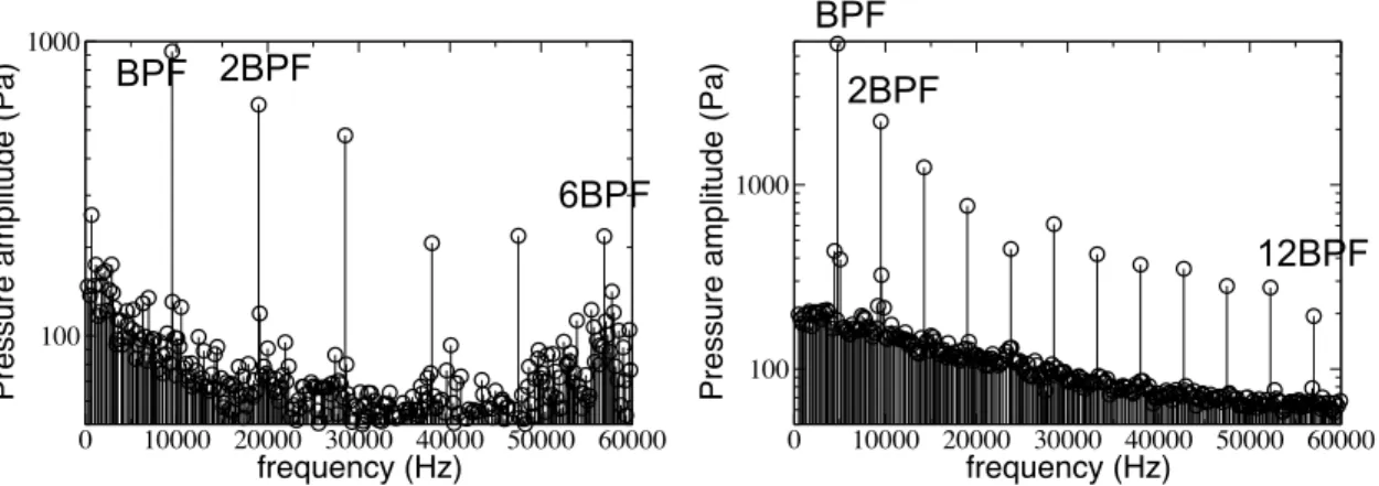
Before analyzing combustion noise generated in the forced case, DMD is performed for the steady inflow case to evaluate the principal sources of activity in the MT1 turbine. Figures 5.15 and 5.16 show the DMD temperature and pressure spectra of the flow in the stator (left) and rotor (right) domains (azimuthal cuts) for the unforced LES. Note that for this specific configuration, the BPF is 9.5 kHz and 4.75 kHz respectively in each domain. The depicted frequency range is 0-60 kHz, which corresponds to the sixth harmonic of the BPF for the stator and the twelfth for the rotor. It is evident both in the temperature and pressure spectra that the rotor/stator interactions are dominant, with the highest peaks located at the BPF of each domain and its harmonics. The second frequency band characterized by increased amplitudes is observed around the sixth harmonic of the BPF for the stator domain. These modes are related to the vortex shedding and the acoustic waves generated from the stator trailing edge. The corresponding mode (12 BPF) in the rotor domain is much weaker. The spatial structure of the BPF mode for each domain (9.5 kHz and 4.75 kHz), along with the common 57 kHz mode (6 BPF for the stator and 12 BPF for the rotor domain) can be visualized to identify the areas of highest amplitudes.
Figure 5.17 shows the temperature and pressure modulus and phase of the BPF mode at mid-span for each domain. In the stator domain, the highest amplitude both for pressure and temperature occurs near the suction side and close to the trailing edge (position 2 in Figs. 5.17(a) and 5.17(c)). This area of the blade is the closest to the passing rotors and thus experiences the largest fluctuations. The fluctuations originating in this area do not stay confined but also propagate upstream, principally through the stator suction side (position 1). In the rotor domain, the BPF corresponds to the rotor blades encountering the passing wakes from the stators. From the temperature and pressure phases, Figs. 5.17(b) and 5.17(d), it can be seen that at the rotor inlet (position 3) the
0 10000 20000 30000 40000 50000 60000
frequency (Hz)
100 1000
Pressure amplitude (Pa)
0 10000 20000 30000 40000 50000 60000
frequency (Hz)
100 1000
Pressure amplitude (Pa)
2BPF 6BPF BPF BPF 2BPF 12BPF
Figure 5.16: DMD pressure spectrums of the stator (left) and rotor domain (right) at mid-span - Steady inflow case.
wake comes at a very high angle, almost perpendicular to the axial direction as the phase changes in the azimuthal direction and stays constant in the axial one. As we go through the rotor passage the flow is turned by the blades and exits the passage with a much shallower angle (position 4).
The temperature as well as pressure modulus and phase of the 57 kHz mode (6 BPF and 12 BPF for the stator and rotor respectively) are depicted in Fig. 5.18. The principal area of activity is the stator trailing edge, where strong acoustic waves are generated. These waves are linked to the oscillating shear layers issued by vortex shedding from the stator wake. The waves generated on the pressure side propagate towards the suction side of the neighboring blade (position 1), while the ones formed from the suction side shear layer tend to move upstream (position 2). It is worth noting though that this activity appears to be largely confined between the stator blades. These observations obtained from DMD seem to match well the phenomena observed in Fig. 5.13(a), position C. In the rotor domain, as seen in the spectra of Figs. 5.15 and 5.16, the e↵ect of the waves is largely attenuated with only the trailing edge showing noticeable amplitude.
DMD results of the forced case
Figures 5.19 and 5.20 show respectively the DMD temperature and pressure spectra of the flow in the stator (left) and rotor (right) domains (azimuthal cuts) for the stationary and forced LES. The depicted frequency ranges of Figs. 5.19 and 5.20 cover up to a frequency equal to the BPF (as seen in each domain) plus the forced Entropy Wave Frequency (EWF) 2 kHz. For the steady inflow case, Figs. 5.19 and 5.20 reveal that there is no mode at the pulsation frequency. For the forced LES, pure entropy waves are injected which create a distinctive peak in Fig. 5.19, seen both in the stator and rotor domains. Furthermore and although no acoustic forcing is imposed by the entropy waves, Fig. 5.20 reveals that a pressure mode with a distinctive peak appears at the forcing frequency. This indicates that acoustic waves have been generated, confirming the
1
1
3
4
3
4
1
1
(a
)
(b
)
(c)
(d
)
2
2
2
2
Figure 5.17: DMD BPF mode at mid-span - Modulus and phase of the temperature (a and b) and pressure (c and d) respectively.
(c)
(b
)
(a
)
(d
)
1
1
1
1
2
2
3
3
Figure 5.18: DMD 57 kHz mode at mid-span - Modulus and phase of the temperature (a and b) and pressure (c and d) respectively.
0 2000 4000 6000 8000 10000 12000 frequency (Hz) 0.1 1 10 Temperature amplitude (K) EWF BPF +EWF BPF-EWF BPF 0 1000 2000 3000 4000 5000 6000 7000 frequency (Hz) 0.1 1 10 Temperature amplitude (K) BPF +EWF BPF-EWF BPF EWF
Figure 5.19: DMD temperature spectra of the stator (left) and rotor domain (right) at mid-span - Steady inflow case ( ) and pulsed case (⇥).
0 2000 4000 6000 8000 10000 12000
frequency (Hz)
100 1000
Pressure amplitude (Pa)
EWF BPF-EWF BPF BPF +EWF 0 1000 2000 3000 4000 5000 6000 7000 frequency (Hz) 100 1000
Pressure amplitude (Pa)
EWF
BPF-EWF BPF
BPF +EWF
Figure 5.20: DMD pressure spectra of the stator (left) and rotor domain (right) at mid-span - Steady inflow case ( ) and pulsed case (⇥).
indirect noise generation mechanism. The imposed EWF also leads to the appearance of interaction modes between the BPF and this forcing with noticeable pressure peaks arising at BP F ± EW F . This type of interaction between combustion noise and rotor/stator tones, yielding scattered tones, has also been measured on full scale engine tests [193].
The mode of primary interest obtained by DMD corresponds to the one at the EWF. Its spatial form can be visualized to identify the spatial activity at the origin of the EWF pressure peak present in Figs. 5.19 and 5.20. The modulus and phase of temperature, as well as pressure of the DMD mode are depicted in Fig. 5.21 at mid-span. The temperature modulus at the inlet, Fig. 5.21(a), is almost uniform and equal to 20 K, corresponding to the plane entropy waves injected in the domain. The phase at the same position, Fig. 5.21(b), indicates that the waves in this area are simply convected by the flow and remain planar. Further downstream in the blade passage, the modulus gets distorted with a reducing maximum value as found in previous 2D propagation studies in a stator [18] and in a turbine stage [189]. The phase also reveals an asymmetric distortion of the planar waves. This distortion is caused by the strong flow acceleration and turning
imposed by the blades. An azimuthal component of the velocity vector is created, with the higher velocity near the suction side resulting in an asymmetric propagation velocity across the azimuthal coordinate. In the rotor domain, due to the rotation the blades see rather uniform entropy waves, with the phase at the rotor inlet being practically planar and perpendicular to the axial direction. As these waves pass through the rotors, they get deformed in a similar fashion as in the first blade row. Such strong distortions of the injected entropy wave at both the stator and the rotor lead to scattering in additional azimuthal modes [18]. This energy redistribution mechanism can explain the additional peaks observed in the pressure and temperature spectra of Figs 5.19 and 5.20.
As anticipated in the discussion based on Figs. 3 and 4, convected temperature spots produce pressure waves in both blade rows at the forcing frequency. The pressure modulus and the phase of the DMD mode at EWF, pictured in Figs. 5.21(c) and 5.21(d), reveal a complex pressure field. A significant peak of the modulus exists between the suction side at 20% chord length and the trailing edge on the pressure side, as the domain is periodic in the azimuthal direction (position 1). In this area the phase hardly changes, Fig. 5.21(d), suggesting an excited cavity mode that stays confined between the blades, making it irrelevant to combustion noise where only propagating waves are of interest. The second area of high pressure modulus can be observed on the suction side close to the trailing edge (position 2), with the sharpest peak corresponding to a shock. In the rotor domain, both the pressure modulus and phase appear to simply follow the flow, with a smooth change of phase throughout indicating simple wave propagation. To finish, a large peak in the pressure and temperature modulus at the trailing edge of the blade corresponds to another trailing edge shock (position 3). At the outlet, the acceleration of the temperature spots through the rotor as well as the acoustic waves generated in the stator and transmitted in the rotor are strong enough to yield a significant pressure trace (non-zero modulus) that sticks above the broadband level. All these features identified in the stator and rotor domains are at the root of the indirect combustion noise emitted and will be quantified later in this work.
Convergence of the DMD
One of the advantages of DMD is the quick convergence of the method, particularly when dealing with oscillatory motions [188, 194] as shown in the 2D test case. The case of 3D turbine stage, however, is much more complex. While the phenomenon of interest consists of oscillating acoustic and entropy waves of known frequency, it coexists with broadband turbulence, shocks, blade wakes, boundary layers and secondary flows that might alter the convergence of the DMD in terms of temporal resolution and overall length of the treated simulations. To evaluate this potential source of uncertainties, DMD on the pulsed case at mid-span is performed with a varying number of snapshots and the same constant sampling frequency, i.e the length of the simulation is modified.
Figures 5.22 and 5.23 depict the DMD temperature and pressure spectra of the pulsed case for five di↵erent simulation runtimes, each equal to a multiple of the period T = EW F1 , which relates to the primary frequency of interest in this work. The sampling frequency for the snapshots is constant and equal to 120 kHz, as in the previous section. The first
2
1
3
1
2
3
1
(b
)
(a
)
(c)
(d
)
Figure 5.21: DMD 2 kHz mode at mid-span - Modulus and phase of the temperature (a and b) and pressure (c and d) respectively
0 2000 4000 6000 8000 10000 12000 Frequency (Hz) 0,1 1 10 Temperature amplitude (K) 1T 3T 6T 8T 10T 0 1000 2000 3000 4000 5000 6000 7000 Frequency (Hz) 0,1 1 10 Temperature amplitude (K) 1T 3T 6T 8T 10T EWF EWF BPF BPF BPF- EWF BPF-EWF BPF+ EWF BPF+ EWF
Figure 5.22: DMD temperature spectrums of the pulsed case with di↵erent number for di↵erent runtimes - stator (left) and rotor domain (right) at mid-span.
0 1000 2000 3000 4000 5000 6000 7000 Frequency (Hz)
100 1000
Pressure amplitude (Pa)
1T 3T 6T 8T 10T 0 2000 4000 6000 8000 10000 12000 Frequency (Hz) 100 1000
Pressure amplitude (Pa)
1T 3T 6T 8T 10T EWF EWF BPF BPF BPF-EWF BPF- EWF BPF+ EWF BPF+ EWF
Figure 5.23: DMD pressure spectrums of the pulsed case with di↵erent number di↵erent runtimes - stator (left) and rotor domain (right) at mid-span.
conclusion that can be drawn is that for the EWF amplitude there is good agreement for all runs with a duration above 3T . For a run time of 1T , EWF in the stator is found to be shifted to slightly above 2 kHz, while in the rotor domain no mode at 2kHz is present. Regarding the BPF mode, a relatively good agreement is also observed, particularly for runtimes above 6T . Most di↵erences appear for the interaction modes BP F ± EW F , where a trend of reduced pressure amplitudes appears as the run-time increases. Regarding the overall spectra, it can be observed that, as more snapshots are added to the signal, the amplitudes of the modes with irrelevant frequencies drop. This indicates that non-coherent broadband phenomena, such as turbulent fluctuations, are present and should not be interpreted as coherent or significant modes. For the cases with 1T and 3T of total runtime, for example, there are several notable peaks that either disappear or are largely reduced when more snapshots are added. Note that for the EWF, where combustion noise will occur, 6 periods T of run-time and above appear adequate for the method to converge.
These results highlight that DMD is more robust when treating purely coherent peri-odic phenomena. Its use in fully turbulent flows, with stochastic fluctuations and broad-band noise present, makes the method prone to reveal more coherent modes than actually present. These flows, therefore, require longer runtimes compared to basic test cases to eliminate such discrepancies. To alleviate this shortcome, a modified version of DMD, called Sparsity-Promoting DMD has been recently developed [195].
Sparsity-Promoting DMD
The spectra of Figs. 5.19 and 5.20 reveal that several other modes are also present around the EWF. Combining this with the fact that the amplitudes of irrelevant modes can require a large amount of snapshots for convergence, it is desirable to be able to evaluate the most important contributions in terms of noise generation and eventually clean up the spectra. To do so automatically a modified version of the DMD has been developed [195] and called the Sparsity-Promoting DMD (SPDMD). This advanced version of DMD aims at selecting the long-standing coherent modes that generate noise while removing the fast decaying ones, typically present because of turbulence, by employing a user-defined regularization parameter that controls the balance between accuracy and a dataset with a reduced set of modes.
In the following, the SPDMD is performed on pressure using the same set of in-stantaneous flow fields as in the previous sections, to identify the most important noise-generating modes in the flow. The intention of this analysis is to verify that this optimized method will recover the pulsation mode and confirm its significance. Figure 5.24 depicts the original pressure DMD spectrum with all the modes present complemented by the sparsity-promoting spectrum superimposed for the turbine inlet and outlet respectively. Both diagnostics provided in Fig. 5.24 are measured at the x-normal inlet and outlet planes for the pulsed case, as it is where the combustion noise will be measured. It can be seen that at the stator inlet the algorithm keeps only the pulsation mode, as expected. At the rotor exit, even though many more modes exist (caused by the local high turbu-lence levels), the mode corresponding to the BPF and the pulsation frequency are chosen
2000 4000 6000 8000 10000 12000 100
102 104
frequency (Hz)
Pressure amplitude (Pa)
EWF
1000 2000 3000 4000 5000 6000 7000 102
103
frequency (Hz)
Pressure amplitude (Pa) EWF
BPF
Figure 5.24: SparsityPromoting DMD at the stator inlet (left) and rotor outlet (right) -Original DMD modes ( ) and SPDMD selected modes (⇥).
as the most coherent ones. It can further be noted that the algorithm retains the EWF mode despite its weak amplitude.
These findings confirm the importance of the indirect combustion noise with respect to other flow phenomena, as well as the ability of DMD to extract it. It also shows that SPDMD can be an appealing method for the analysis of real combustors. With realistic entropy waves generated at flame fronts being broadband and not monochromatic, such a method has the potential of quickly identifying the entropy modes that are most probable to generate indirect noise and thus provide more guidance for the design. However, in this monochromatic study the frequency of the indirect noise is known a priori, as it corresponds to the user-defined EWF so the standard DMD method is sufficient.
5.5.3
Quantifying the indirect noise and comparisons with the
compact theory
The noise that is measured in this study is the result of a pulsated, realistic 3D turbine with several flow features present (notably the secondary flows at the hub and casing of the stator, the tip leakage flow at the rotor, the complete 3D shock structures and the shock-boundary layer interactions). In terms of noise generation, it can be compared with the 2D compact theory of Cumpsty and Marble [38]. Numerical results from 2D pseudo-LES (using the MISCOG approach and a simple mesh deformation technique) of a simplified turbine stage described in detail in [189] serve as an additional complement to the theory and the full 3D simulations. It is worth noting that Duran et al. [34] commented that for his configuration (a modified version of the MT1 turbine stage at mid-span with a 30:30 blade count) 2 kHz is approximately the limit after which the compact assumption is not valid.
To measure the transmission of the generated acoustic waves, DMD is performed at the inlet and outlet x-normal planes. Assuming that at these locations the waves are 1D plane waves, the downstream propagating acoustic wave can be calculated as
w+= p0
p + u0
c , the upstream propagating acoustic wave as w = p0
p u0
c and the entropy wave ws= p0
p ⇢0
⇢. The overline in these expressions indicates time averaged quantities, the prime indicates fluctuations and the heat capacity ratio is assumed to be constant throughout, while u indicates the axial component of the velocity. The formulation of these waves is dimensionless. The transmission coefficients of interest are the entropy wave attenuation T s = ws2
ws
1, the acoustic wave reflection Ra =
w1 ws
1 and the acoustic wave
transmission T r = w+2
ws
1, with the subscript 1 indicating the turbine inlet. The subscript 2
refers to the turbine outlet and ws
1 is the forced entropy wave imposed at the inlet. The procedure to construct the characteristic waves and measure the transmission coefficients at the inlet and outlet of the turbine stage can be decomposed into 5 steps:
1. Perform DMD of the principal flow variables at an x-normal plane both at the inlet and outlet of the turbine.
2. Isolate the mode of interest (EWF in this case) and form the temporal fluctuations of the variables.
3. For each point in the plane construct the 1D plane waves using the reconstructed fluctuations and a time-averaged solution.
4. Perform surface averaging and calculate the transmission coefficients.
Applying this procedure at the inlet of the turbine stage is straightforward, since there is no free-stream turbulence imposed. However, as the flow goes through the turbine it generates broadband fluctuations. While DMD allows an easy filtering of all irrelevant frequencies, turbulence or hydrodynamic phenomena whose frequency coincides with the pulsation frequency will be present in the signal and can therefore modify the evaluation of the transmission coefficients. As a result, at the rotor outlet an extra step is added before step (4): a hydrodynamic filtering based on the Characteristics Based Filtering (CBF) method [196] is applied to separate hydrodynamics from acoustics knowing their di↵erent propagation velocities. To apply this filtering, the waves are measured in 3 outlet x-normal planes in close proximity (instead of just 1). The Taylor hypothesis and the known wave speed are then used to correlate the data between the 3 planes at di↵erent physical times following the formula:
wa = 1 3 2 X i=0 f (x i x, t i x up ) (5.7)
In Eq. (5.7), f is the wave of interest, wa is the filtered wave, x is the distance between the planes and up is the wave speed, i.e u + c for w+ and u for ws.
Results, obtained with the procedure described above, are summarized in Fig. 5.25, where they are also compared to the theory and 2D numerical predictions. For the com-pact theory and 2D simulations, predictions across a broad frequency range are available. The 3D predictions are close to the 2D ones, while the compact theory predicts stronger upstream propagating generated noise and slightly lower transmitted noise. Regarding
the entropy wave transmission, the results of the 3D simulation suggest that at the tur-bine outlet the injected wave has been dissipated more than in the 2D simulations, while the theoretical approach neglects the entropy wave attenuation process. Concerning the acoustic waves generated at the forcing frequency, for the downstream propagating acous-tic wave, the two numerical simulations are in reasonable agreement. For the upstream propagating wave, the 3D simulation predicts a small decrease in strength compared to the 2D prediction, probably because of the choked operating condition that prevents acoustic waves generated downstream the sonic line to travel towards the turbine inlet.
5.6
Conclusions
In this chapter, the indirect combustion noise generation mechanism across a pressure turbine has been investigated. It is achieved by performing LES of a 3D high-pressure turbine stage subject to a constant-frequency entropy wave train pulsation. To simplify the data processing, the flow field and the generated noise are analyzed through the Dynamic Mode Decomposition of instantaneous snapshots at several positions across the turbine and the results are compared with a steady inflow case. When no wave forcing takes place, the strongest noise-generating mechanisms are revealed to be the rotor/stator interactions occurring at the BPF and its harmonics, followed by weaker activity due to the stator vortex shedding and trailing edge acoustic wave generation. When entropy wave injection is activated, a distinctive high-amplitude mode at the pulsation frequency is generated, as well as interaction modes with the blade passing frequency. The influence of the entropy waves is also captured by the sparsity-promoting DMD, a modified DMD algorithm that provides an accurate reconstruction of the flow field with few well-selected modes. Despite the presence of broadband turbulence and non-linear interactions, the blade passing frequency and pulsation modes are shown to be the most important ones. For the forced frequency, a detailed analysis of the 3D LES predictions is performed and the results are compared with the compact theory [38] as well as 2D simulations of a similar turbine configuration. While the theory overpredicts the noise levels, the 3D LES of the choked transonic HP turbine reveals that the entropy waves get highly distorted and weaker as they are transmitted to the following stages if compared to 2D results or the compact theory (unlikely to generate any additional indirect noise). The transmitted acoustic waves to the consequent stages remain strong, and will equally contribute to the indirect noise as in the 2D simulations. The reflected acoustic waves are slightly weaker than in 2D predictions and much more attenuated than in the compact theory.
This chapter also serves as the first application of MISCOG on a combustion chamber-turbine interaction problem. While the problem is treated in a decoupled fashion from the combustor, the method proves to be capable of capturing the complex generation mechanisms of indirect combustion noise in a fully 3D high-pressure turbine stage where rotor/stator interactions are important. These results, thus, can provide some degree of confidence that the method is capable of treating a fully coupled combustion chamber-turbine problem.
LES - 0.09
LES - 0.018 LES - 0.017
(a)
(b)
(c)
Figure 5.25: Transmission coefficients - a) Ra b) Tr and c) Ts - Compact theory (solid line), 2D simulations (+ and•) and LES (•)
LES of an industrial combustion
chamber-turbine system
Contents
6.1 Multicomponent simulations of gas turbines . . . 122 6.2 Hot-streak migration across turbines . . . 125 6.2.1 Segregation e↵ect . . . 125 6.2.2 Other parameters influencing the hot-streak migration . . . 126 6.3 LES of an industrial high-pressure turbine stage . . . 129 6.3.1 Standalone turbine geometry . . . 129 6.3.2 Mesh . . . 130 6.3.3 Boundary conditions . . . 132 6.3.4 Numerical setup and initialization . . . 133 6.3.5 Results . . . 133 6.4 Fully coupled combustion chamber-turbine simulation . . . 141 6.4.1 Geometry . . . 141 6.4.2 Mesh . . . 142 6.4.3 Combustion modelling . . . 142 6.4.4 Initialization and numerical set-up . . . 144 6.4.5 Results . . . 146 6.5 Conclusions . . . 152
In this chapter, the MISCOG method is used to perform combustor-turbine LES of a helicopter engine, the focus being placed on the aerothermal interactions in such systems. Before presenting the numerical simulations, the literature on previous multi-component simulations of gas turbines and on the migration of combustor-generated non-uniformities across turbines is reviewed. Although the main objective here is to illustrate the capacity of MISCOG to treat the full combustor-turbine LES flow of real industrial configurations, the turbine is first investigated alone. Comparatively to the simulations of Chapter 4, increased fidelity is introduced by imposing realistic time-averaged temperature profiles at the inlet of this standalone turbine LES, provided by an existing LES of the combustion chamber. Comparisons of the aerodynamic flow field with standard steady-state RANS simulations that employ the cheaper mixing plane method for the rotor/stator interface (provided by Turbomeca) permits the comparison of the results of this first complex turbine stage LES with the typical industrial simulation method.
The second part of this chapter is dedicated to a fully coupled, multi-species and reactive LES of the entire combustion chamber-HPT system. With this approach, all the heterogeneities at the combustor outlet can be propagated in real time through the turbine, thus taking into account all combustor-turbine interactions in time and space. This last simulation highlights the potential of the developed methods for future multi-component simulations of gas turbines and is compared to the standalone turbine LES. Although such predictions remain at this stage preliminary and clearly require further e↵orts, both simulations are compared with a focus on the migration of temperature non-uniformities across the entire turbine stage.
Note that a large part of the presented simulations was performed during a 3-month secondment at Turbomeca, in the frame of the project COPA-GT. For confidentiality reasons, figures that include temperature and pressure have been normalized by the total temperature and total pressure at the turbine inlet issued by the thermodynamic cycle of the engine.
6.1
Multicomponent simulations of gas turbines
The advantages of coupled multi-component simulations, complemented with the in-creasing computational resources, have sparked considerable interest since the beginning of 2000’s. A first full engine simulation was produced for the General Electric GE90 engine by Turner et al. [19] within the NASA Numerical Propulsion System Simulation (NPSS) program. For this simulation, dedicated solvers for each component were used, the unstructured National Combustion Code for the combustion chamber [197] and the structured multi-block APNASA code for the turbomachinery stages. Both codes are steady-state RANS solvers employing the k ✏ turbulence model [198]. This work relied on a turbomachinery-combustor coupling method developed earlier [199, 200] which en-sured mass and total enthalpy conservation and resulting e↵orts were oriented towards the capacity of such a tool to recover the main cycle parameters of the engine. Despite the success of the simulation in capturing such engine data (Fig. 6.1 presents the error on the prediction of the main thermodynamic parameters across the engine compared
to experimentally measured values), the RANS approach and the modeling of significant technological e↵ects, such as the tip clearances of the rotating machineries or coolant injections, were found to impact the predictions significantly [201].
Figure 6.1: Full GE90 simulation comparison to engine cycle data. Percent di↵erence in total pressure (P), total temperature (T) and flow rate (W) from experimentally measured values [19].
Figure 6.2: LES/RANS interface at the compressor exit with turbulent fluctuations superim-posed at the time averaged RANS solution [20].
To increase the fidelity of such multicomponent tools, combustor simulations switched to solvers based on the LES formalism, considered more accurate than RANS for this com-ponent [202]. For the wall-bounded high-Reynolds turbomachinery parts, the (U)RANS approach was retained. The most notable work using this type of coupling was the full engine simulation performed at Stanford University in the framework of the ASCI project [20, 21]. The principal challenge with this di↵erent approach is in the handling of the interfaces between the di↵erent solvers and formalisms: a) at the RANS/LES inter-face, located at the compressor exit, turbulent fluctuations need to be reconstructed and
injected in the LES domain and b) the LES/RANS interface placed at the turbine inlet needs a specific treatment to ensure a smooth transition and conservativity. Difficulties were also added due to the fact that the combustion chamber solver was incompressible compared to the compressible turbomachinery solver.
LP/HP%compressor%
interface% HP/LP%turbine%interface%
Figure 6.3: View of the high-pressure flow field from the full engine simulation (top) and radial pressure profiles at two di↵erent engine positions (bottom)[21].
For the reconstruction of turbulent fluctuations at the RANS/LES interface, Medic et al. [20, 203, 204] proposed a recycling technique. In this approach the turbulent fluctuations are calculated in parallel ”on the fly” by a periodic duct LES with similar conditions as those prevailing at the combustor inlet. Obtained fluctuating fields were then superposed to the time averaged RANS profile and used at the LES inlet, Fig. 6.2. On the other side of the combustion chamber, to overcome the difficulties between the incompressible-compressible solver coupling, Schl¨uter et al. [205, 206] proposed the use of the body force method: the LES domain has an overlapping region with the RANS domain and within this region the mean velocity of the LES solution is driven towards the RANS solution with the addition of body forces. The final full engine simulation, combining LES and RANS, depicted very realistic flow fields and the existing measurements for the pressure radial profiles at two di↵erent engine locations (low-pressure/high-pressure
Figure 6.4: Typical combustor outlet temperature profile [22].
compressor interface and the corresponding turbine interface) showed a generally good agreement with the simulation, Fig. 6.3.
6.2
Hot-streak migration across turbines
As mentioned in Chapter 1, the combustion chamber generates temperature hetero-geneities, turbulence and swirl that propagate and migrate across the turbine stage. Figure 6.4 depicts a typical time-averaged temperature profile at a combustor exit high-lighting the large temperature di↵erences across the sector. The thermal load of the blade rows, already constrained by the high mean operating temperatures, is altered con-siderably by these heterogeneities. This necessitates consequently a good prediction of the migration of the non-uniformities if an optimal design of the blade and its cooling systems is to be obtained. The importance of the combustor-turbine interactions can be better highlighted if one considers that an under-prediction of the blade temperature by just 15 degrees (when the inlet temperatures are well over 1500 K) can reduce the expected life duration of the turbine by half. Note that di↵erent physical e↵ects and features are important on the migration of temperature heterogeneities across turbine stages, as detailed below.
6.2.1
Segregation e↵ect
An important consideration when trying to predict the migration of temperature non-uniformities in the rotor blades of a turbine stage is the segregation e↵ect first described in [207]. If the Mach number and flow angles are considered constant, fluid of higher temperature will have an increased absolute velocity at the stator exit due to the increased speed of sound, while cold gases will be slower. As a result, when the rotational velocity
Cold gases Hot gases U
Stator
Rotor
Relative velocityFigure 6.5: Schematic showing the segregation e↵ect.
is added at the stator/rotor interface, the relative velocity angle seen by the rotor blades is di↵erent as illustrated in Fig. 6.5. While for both hot and cold gases the flow angle of the absolute velocity is the same, the higher magnitude of the hot gas velocity creates a relative velocity with a higher angle and magnitude. In real turbines with hot streaks, this leads to a preferential migration of the hot gases towards the pressure side of the rotors as confirmed experimentally by Butler et al. [208]. An interesting thing to note is that this phenomenon is fully unsteady. As a result, predictions from steady-state numerical simulations, which are prevalent at the design stage of a turbine, cannot take such e↵ects into account.
6.2.2
Other parameters influencing the hot-streak migration
Figure 6.4 depicts a hot spot located in the center of the sector and contained between 40 and 60% of the span. This specific alignment of the non-uniformities can be however altered by the relative placement of the fuel injectors and the dilution holes present in the combustion chamber. As a consequence, a lot of research has been performed to evaluate the e↵ect of the azimuthal and radial placement of hot-streaks on the resulting temperature profiles across the blade passages. Additional flow characteristics at the turbine inlet are also know to a↵ect the heat load on the blades. Among others, the free-stream turbulence and length scales along with the residual swirl from the combustor are of crucial importance.
• E↵ect of the fuel injector and vane clocking
The principal parameter in hot-streak migration is considered to be the azimuthal placement, also called clocking, of the hot spots with respect to the blade leading edge.
Leading edge alignment Mid-passage
alignment
Figure 6.6: E↵ect of clocking on the NGV heat load [15].
Povey et al. [15] performed a numerical and experimental investigation of the e↵ect. A significant increase in the heat transfer on the suction side of the stator (also called Nozzle Guide Vane, NGV) was observed when the hot part was aligned with the blade leading edge, while aligning the hot streak with the blade passage was reducing it, as shown in Fig. 6.6. Although the latter alignment can be beneficial for the stators, it can prove to be damaging for the rotor if the segregation e↵ect is taken into account. In realistic geometries, the distance between blade rows is small and the flow at the outlet of the stator is not uniform. The wake region has a velocity deficit compared to the free-stream. Aligning the hot flow with the leading edge would direct the hotter, higher velocity gas in the wake region, reduce the velocity deficit and help cancel the segregation e↵ect. As a result, the heat load on the rotor pressure side can be reduced. This has been confirmed by He et al. [26], in a thorough study of di↵erent hot-streak counts in the heat loads across the MT1 turbine stage.
• Impact of the hot-streak radial position
Besides the azimuthal placement of the non-uniformities, there is also evidence of the importance of the radial position of hot-streaks. In fact, small contained hot-streaks around mid-span are shown to have little impact on the blade heat load close to the endwalls. More specifically, Povey et al. [15] observed a decrease of the heat load as the temperature is decreased locally near the endwalls. On the contrary, when hot-streaks are enlarged they can interact with the secondary flows, the passage vortices being able to transport hot, high-energy fluid from the free-stream towards the hub and casing boundary layers, thus increasing the heat load at these locations [29]. Similar conclusions were drawn by Roback and Dring [28], when the position of the hot streak is moved radially towards either the hub or the casing. Finally, note that additional radial