Chapter 9
Test case C: industrial
configuration
This final chapter deals with the application of mesh adaptation (described in chapters 5-8) to the industrial configuration studied in the first part of this thesis. This chapter bridges the two parts that compose this manuscript. Here, mesh adaptation is tested on the fixed swirler configuration (left in Fig. 2.1) studied in chapter 3. For the fixed swirler case, it was proven that the mesh has a significant influence on LES results because of its impacts on turbulent viscosity (Eq.(3.6)) and because of the numerical noise induced by a locally under-resolved flow. These effects, whose magnitude depends on the particular SGS model used, are able to modify the flow speed locally and these local modifications bring about a global flow bifurcation because of critical conditions1. However, two issues remain open from chapter 3:
1. results did not match experimental data perfectly, both in terms of the jet opening half-angle and of the length of the recirculation zone (Fig. 3.20) even when an opti-mized mesh2 was employed and despite the fact that LES predicted the same flow state (Axial Jet, see chapters 3-4) of the experiment3;
2. pressure drop was over-predicted compared to experimental data ranging from a at least +66% to a at most +160%, depending on the SGS model used (Fig. 3.22). The challenge of mesh adaptation here is therefore to improve comparison with experi-mental data in terms of velocity profiles and pressure drop predictions.
Most of the mesh related issues of chapter 3 came from the interaction wall resolution/SGS modeling. For instance, SGS modeling was proven to modify the amount of swirl in the flow and to cause a change in the flow topology (sections 3.4-3.5) while this phenomenon disappeared when mesh resolution was increased in the wakes of the radial swirler blades and inside the vane itself (see section 3.7).
Regarding pressure losses, results of Barre et. al [7] show that pressure drop error can be reduced from +105% to +52% with respect to experimental data by reducing the y+ of wall elements from O(60) to O(15) (i.e. refining the mesh at the wall). This result can be
1This second statement was proven in chapter 4. 2
Optimized based on fluid dynamics considerations, see section 3.7, Fig. 3.16 right. 3See section 2.2.3 and section 3.6
9.1. MESHES AND NUMERICAL SETTINGS 171 considered as ”obvious” since dissipation for bounded flows is governed by the boundary layer physics and, since LES equations are consistent with the Navier-Stokes equations, a higher resolution in the boundary layer should improve results. Similarly, the scaling of turbulent viscosity with the distance to the solid boundary affects pressure drop.
Finally, as mentioned in the introduction, as soon as a swirler with multiple passages is used, any error on pressure losses will directly impact on the flow split between the pas-sages, leading to significant flow variations.
For all these reasons, mesh adaptation is targeted toward wall resolution in order to study the effects of the error distribution between the different swirler vanes on the global flow field generated by the swirler.
9.1
Meshes and numerical settings
The metric field (see chapter 6) used for mesh adaptation in this chapter is based on y+ (Eq. 3.1), the wall distance in wall units. This choice is motivated by the fact that wall resolution is of importance for flow split and pressure drop and because the use of any of the sensor field used in the previous Chapters would have required some ad-hoc adjustments. The reason is simple: while in Chapters 7-8 confined flows were simulated (as usually happens at CERFACS with gas turbines combustion chambers) the jet examined here blows in open atmosphere. Here, in the far field, all sensors previously tested (such as turbulent viscosity or resolved turbulent kinetic energy) are high because of the coarse mesh used4.
On the other hand, a sensor based on the velocity gradient would cluster all nodes close to the swirler walls because of high shear present in this zone, obtaining a mesh similar to the one proposed in this chapter. However, while adapting the mesh based on y+ is possible to choose how well we want to resolve the boundary layer (by adjusting the target y+), choosing the velocity gradient, grid resolution would have been controlled by the constraint on minimum mesh size (the sensor generator would impose very small elements at the wall while the constraint on the minimum cell size would limit their size, see section 6.2.2). A sensor based on y+ helps to skip all these problems fast and allows to test directly the mesh adaptation on the industrial configuration studied in the first part of this manuscript. This approach is in line with the mesh adaptation strategy explored in this thesis: any category of flow (such as ”round jets” of Chapter 7) has its own peculiarities and requires a targeted mesh adaptation method.
The metric field is built as follows:
M (x) = 1 (h(x)s(x))2 0 0 0 (h(x)s(x))1 2 0 0 0 (h(x)s(x))1 2 (9.1)
where M (x) is the local metric at a position x = (x1, x2, x3), h(x) is the local mesh size of the original mesh to be adapted, s(x) is a scaling factor. The value of the scaling factor s
4
A coarse mesh in this zone is justified by the fact that the flow in the open atmosphere has a limited effect on the jet dynamics compared to flow inside the swirler or at the nozzle, see Chapters 3-4
172 CHAPTER 9. TEST CASE C is evaluated as follows: s(x) = ( y+ T y+ at the walls, 1 else, (9.2)
where y+T is the desired target value of y+ to obtain on the adapted mesh (in this case yT+= 11, that is above the laminar sublayer).
The mesh size gradation (see section 6.2.3) is set to 1.2 in order to smooth the metric field which is by construction (Eq.(9.2)) discontinuous. The metric field built using Eq.(9.1-9.2) has the peculiarity to refine the grid only at the walls while interior cells are, in a first instance, left untouched (s(x) = 1). However, since the number of nodes of the mesh is preserved, a wall-targeted refinement implies a coarsening in the bulk of the flow, therefore no element remains the same after adaptation.
The aim of this sensor field is to equidistribute the size of the wall elements in order to get an homogeneous mesh in terms of y+. The adaptation criterion is very simple: if the local value of y+ of flow computed on the original mesh is smaller than the target value y+
T, the element will be enlarged (s(x) > 1 so h(x)s(x) > h(x) in Eq.(9.1)), on the contrary it will be reduced (s(x) < 1 so h(x)s(x) > h(x) in Eq.(9.1)).
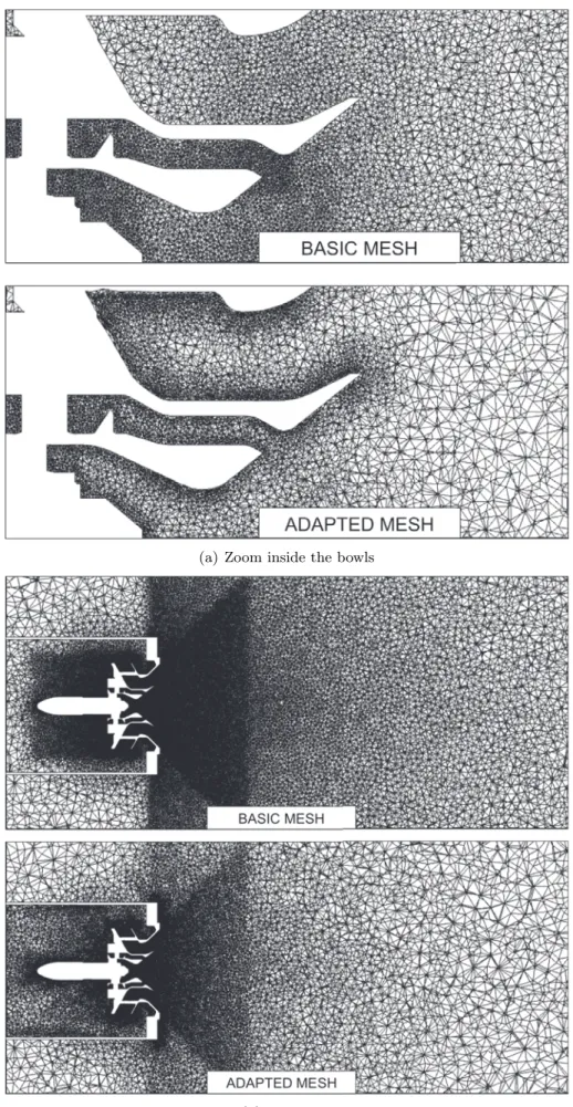
Obviously, such a method requires a LES flow field to compute the local scaling factor s(x). The mesh and flow field chosen as the initial grid and solution are the one of LES YALES-SIGMA of section 3.4 (the mesh is shown in Figs. 3.5(a) and 3.16, ”basic”), which are the worst in terms of comparison with experimental data between all results of chapter 3. The resulting adapted mesh (based on the metric field built using Eq.(9.1-9.2)) is shown in Fig. 9.1(a)-9.1(b) along with the ”basic” mesh used for LES YALES-SIGMA. The adapted mesh (named ADAPTED simply) is refined mainly inside the radial swirler (where the value of y+ is higher) and coarsened away from the wall.
As evident from Fig. 9.1(b), far from the solid boundaries, the ”basic” and ADAPTED meshes are very similar. This is a consequence of the fact that, in these zones, elements of adapted mesh are by construction similar to the elements of the basic mesh (s(x) = 1 in Eq.(9.2)). However, there, in the free jet, the ADAPTED mesh is clearly coarser than the ”basic” mesh (Fig. 9.1(b)). This phenomenon is due to the fact that the overall number of nodes is kept constant (see section 6.2.4). Since the ADAPTED mesh is refined at the walls and, at the same time, the overall number of nodes is conserved, the ADAPTED mesh is coarsened away from the solid boundaries.
The number of nodes and elements of the ADAPTED mesh are 2269213 and 12888044 respectively, similar to the number of nodes/elements of meshes ”basic” and ”optimized” of Fig. 3.16. The boundary conditions used for the test performed in this chapter are the same as in chapter 3 (see Fig. 3.3 and table 3.1). The code used here is YALES2 and the SGS model is the Dynamic Smagorinsky model [29] (see section 3.2.2).
9.1. MESHES AND NUMERICAL SETTINGS 173
(a) Zoom inside the bowls
(b) Zoom out
Figure 9.1: ”Basic” mesh vs. mesh ADAPTED using Eq.(9.1-9.2) and the flow field of LES YALES-SIGMA of section 3.4.
174 CHAPTER 9. TEST CASE C
9.2
Flow field
The ADAPTED LES (the mesh and simulation are both named ADAPTED for simplicity) reaches convergence in terms of kinetic energy after 0.030[s]. Kinetic energy is evaluated inside a box (see Fig. 4.11) big enough to fully contain the recirculation bubble of the Blasted vortex Breakdown state (which is the largest observed, see Chapters 3-4). This choice is motivated by the fact that to obtain the convergence of kinetic energy in the whole simulation domain requires an excessively long simulation time. For comparison, both kinetic energies (evaluated inside the ”box” of Fig. 4.11 and in the whole simulation domain) are shown in Fig. 9.2: kinetic energy inside the box converges fast (as already experienced for LES of chapter 4) while in the whole chamber it keeps on increasing slowly.
0 10 20 30 40 Time [ms] 0,125 0,25 0,5 1 2 4 8 16 32 64 kinetic energy U2, "BOX" U2, "CHAMBER"
Figure 9.2: Instantaneous kinetic energy evolution for LES ADAPTED of table 9.1. Kinetic energy is evaluated inside the ”box” of Fig. 4.11 and in the whole simulation domain. Logarithmic scale.
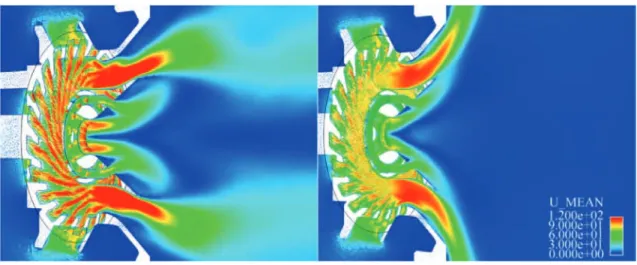
The flow field of LES ADAPTED is compared to the flow of LES of table 3.13, obtained with the optimized mesh of Fig. 3.16 (see section 3.7). The flow field of LES adapted is shown in Fig. 9.3 (together with results of LES YALES-SIGMA O as comparison) while its characteristics, in terms of the three different jets swirl number/ratio (measured on surfaces S1, S2 and S3 of Fig. 3.6 as explained in section 3.3.1) are summarized in table 9.1.
LES S (eq. 2.2) Sr (eq. 2.3) jet
name inner/outer jet radial jet configuration
ADAPTED 0.12/ 0.47 0.76 AJ
YALES-SIGMA O 0.12/0.58 0.74 AJ
YALES-DSMAG O 0.12/0.4 0.72 AJ
AVBP-SIGMA O 0.12/0.52 0.76 AJ
Table 9.1: Fluid dynamics characteristics of LES ADAPTED and of LES of table 3.13.
Under these fluid dynamics conditions (summarized in table 9.1), the flow obtained with the adapted mesh is in the AJ state (as evident from the size of the central recircu-lation zone shown in Fig. 9.4, the pressure and rms profiles shown in Fig. 9.5).
The first difference between LES ADAPTED and LES of table 3.13 (which are used as comparison) is the jet opening half-angle (see Fig. 3.7) which is significantly larger and is the largest obtained in the fixed swirler configuration (Fig. 2.1) for a jet in the AJ state.
9.2. FLOW FIELD 175
(a) ADAPTED
(b) YALES-SIGMA O
Figure 9.3: Mean velocity for two of the LES of table 9.1.
Fig. 9.6 shows the jet opening half-angle for LES ADAPTED and for all LES of table 3.13: LES ADAPTED predicts a jet opening half-angle of 35[deg] very close to the experimental value of 34[deg] and similar to the result obtained with LES basic of section 4.5 obtained on a much finer mesh.
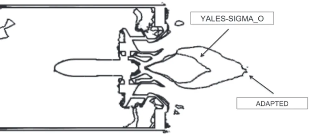
The second remarkable difference is the size of the Central Toroidal Recirculation Zone (CTRZ). As evident from Fig. 9.4 (where the CTRZ of LES YALES-SIGMA O is shown as comparison) the CTRZ is significantly longer.
The different jet opening angles and the size of the CTRZ have a deep impact on the velocity profiles. Figs. 9.7-9.8-9.9 show the velocity profiles of all LES of table 3.13, of LES ADAPTED and compare them with the experimental velocity profiles. Results of LES ADAPTED show a significant improvement with respect to all LES obtained with the optimized mesh, showing a better comparison with experimental data at all planes and for all velocity components. Note that the size of the CTRZ is perfectly matched with the back-flow intensity (Fig. 9.9(a)).
176 CHAPTER 9. TEST CASE C
Figure 9.4: CTRZ for LES of ADAPTED of table 9.1 compared with LES YALES-SGIMA O of table 3.13.
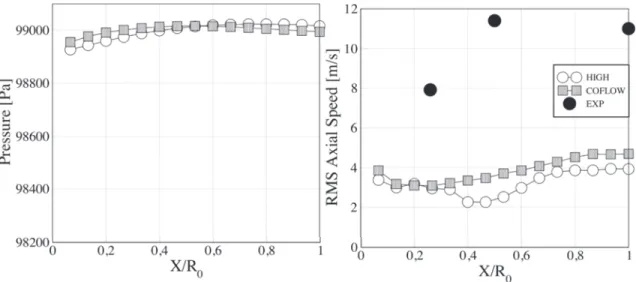
Figure 9.5: Axial velocity RMS and pressure distribution measured along the centerline of the geometry for simula-tions of table 3.13 and LES ADAPTED of table 9.1. Results are plotted against normalized axial distance (X/R0)
from the swirler ending plate. Experimental data are available only for RMS values.
Figure 9.6: Jet opening half-angle (Fig.3.7) for simulations of table 3.13 and LES ADAPTED of table 9.1. Note that LES ADAPTED shows a jet opening half-angle of 35[deg] very close to the experimental data of 34[deg].
9.2. FLOW FIELD 177 0 0,5 1 1,5 2 R/R0 0 20 40 60 80 100 Speed [m/s] YALES-SIGMA_O YALES-DSMAG._O AVBP-SIGMA_O ADAPTED EXP (a) Axial 0 0,5 1 1,5 2 R/R0 -10 0 10 20 30 40 Speed [m/s] YALES-SIGMA_O YALES-DSMAG._O AVBP-SIGMA_O ADAPTED EXP (b) Radial 0 0,5 1 1,5 2 R/R0 0 10 20 30 40 50 60 Speed [m/s] YALES-SIGMA_O YALES-DSMAG._O AVBP-SIGMA_O ADAPTED EXP (c) Tangential
178 CHAPTER 9. TEST CASE C 0 0,5 1 1,5 2 R/R0 -20 0 20 40 60 80 Speed [m/s] YALES-SIGMA_O YALES-DSMAG._O AVBP-SIGMA_O ADAPTED EXP (a) Axial 0 0,5 1 1,5 2 R/R0 -20 -10 0 10 20 30 Speed [m/s] YALES-SIGMA_O YALES-DSMAG._O AVBP-SIGMA_O ADAPTED EXP (b) Radial 0 0,5 1 1,5 2 R/R0 0 10 20 30 40 50 Speed [m/s] YALES-SIGMA_O YALES-DSMAG._O AVBP-SIGMA_O ADAPTED EXP (c) Tangential
9.2. FLOW FIELD 179 0 0,5 1 1,5 2 R/R0 -20 0 20 40 60 Speed [m/s] YALES-SIGMA_O YALES-DSMAG._O AVBP-SIGMA_O ADAPTED EXP (a) Axial 0 0,5 1 1,5 2 R/R0 -20 -15 -10 -5 0 5 Speed [m/s] YALES-SIGMA_O YALES-DSMAG._O AVBP-SIGMA_O ADAPTED EXP (b) Radial 0 0,5 1 1,5 2 R/R0 0 10 20 30 40 50 Speed [m/s] YALES-SIGMA_O YALES-DSMAG._O AVBP-SIGMA_O ADAPTED EXP (c) Tangential
180 CHAPTER 9. TEST CASE C
9.3
Pressure drop and flow split
Flow split changes significantly after mesh adaptation: using the ADAPTED mesh, the mass flow rate through the radial stage increases while the mass flow rate through the axial stage decreases (it reduces by 17% with respect to YALES-DSMAG O, see table 9.2) and differs significantly from permeability measurements.
Mesh adaptation causes a drastic reduction of the pressure drop (table 9.2). Note that table 9.2 compares pressure drop and flow split of LES that have the same SGS model (Dynamic Smagorinsky [29]), since, as proved by Fig. 3.22, pressure drop is mainly a function of the SGS modeling. Using adaptation, the error on pressure drop reduces from +120% of LES YALES-DSMAG O to +70% with the adapted mesh, which still is a large error, but represents a net improvement.
Flow repartition and pressure drop
axial stage radial stage total mass flow pressure drop
EXP 16.5 [g/s] 85.5 [g/s] 102 [g/s] 4800 [Pa]
ADAPTED 13.4 [g/s] 88.2 [g/s] 101.6 [g/s] 8205 [Pa]
YALES-DSMAG O 15.9 [g/s] 86.1 [g/s] 102.0 [g/s] 10657 [Pa]
Table 9.2: Flow repartition and pressure drop for LES ADAPTED of table 9.1. Note that flow split is signifi-cantly different from the experimental value obtained from permeability measurements. However, the accuracy of permeability measurement is questionable.
In order to study the effects of modeling on pressure drop, the SGS model was switched from Dynamic Smagorinsky to SIGMA in the converged flow of LES ADAPTED. Results obtained with this new simulation, labelled ADAPTED S, are summarized in table 9.3. As expected, using the SIGMA SGS model, pressure drop reduces to 6826 [Pa] equivalent to an error of +42 % with respect to experimental data and which is significantly lower than LES YALES-SIGMA O or AVBP-SIGMA O (+80 %). Such an error on pressure losses is even lower than the one shown on Jaegle’s [47] LES on a very similar injector and with a dedicated wall function (+54%).
Flow repartition and pressure drop
axial stage radial stage total mass flow pressure drop
EXP 16.5 [g/s] 85.5 [g/s] 102 [g/s] 4800 [Pa]
ADAPTED S 13.5 [g/s] 88.0 [g/s] 101.5 [g/s] 6826 [Pa]
YALES-SIGMA O 15 [g/s] 87 [g/s] 102.0 [g/s] 8535 [Pa]
AVBP-SIGMA O 15.7 [g/s] 85.8 [g/s] 101.5 [g/s] 8647 [Pa]
Table 9.3: Flow repartition and pressure drop for LES ADAPTED S and LES of table 9.1.
From the analysis of tables 9.2-9.3 it can be argued that the improvements on pressure drop are likely to be linked to a different flow split in the axial and radial stages. This flow split change is due to an equirepartition of the error made at the walls. Fig. 9.10 shows the Probability Density Function (PDF) of the y+in the computational domain for LES ADAPTED and LES YALES-SIGMA (which was used for building the sensor field). Using a mesh adapted based on a target value of y+, this quantity becomes homogeneous in the different stages of the swirler (the Root Mean Square of this quantity reduces almost
9.3. PRESSURE DROP AND FLOW SPLIT 181 by 50%, from 13 in LES YALES-SIGMA to 6.8 with the adapted mesh).
However also the mean y+ value reduces (from 27 in LES YALES-SIGMA to 18 with the adapted mesh) and it is therefore impossible to verify if pressure drop prediction improves because of a lower y+ or because of a change in flow split related to a more homogeneous y+ in the different passages.
0 5 10 15 20 25 30 35 40 45 50 55 60 65 70 75 y+ 0 0,25 0,5 0,75 1 1,25 PDF (%) YALES-SIGMA ADAPTED
Figure 9.10: PDF of mean y+for LES ADAPTED and LES YALES-SIGMA (which was used for building the sensor
field). Using adaptation the y+becomes more homogeneous in the domain (the RMS value of this quantity reduces
from 13 in LES YALES-SIGMA to 6.8 with the ADAPTED mesh) while its mean value reduces from 27 in LES YALES-SIGMA to 18 with the ADAPTED mesh (close to the imposed value of 11). This causes a net improvement of pressure drop prediction and a different flow split.
In order to clarify this issue, a second adapted mesh was generated in which the target y+ (y+T in Eq.(9.2)) was fixed to be twice larger in the radial swirler than everywhere else in the domain. Fig. 9.12 shows this mesh, labelled ADAPTED NH (Non-Homogeneous), which is clearly coarser than the adapted mesh inside the radial swirler. The LES per-formed with this mesh, using the Dynamic Smagorinsky model, predicts a flow split similar to all LES of Chapter 3 (see also tables 9.2-9.3) and a pressure drop error of +100% with respect to experimental data (see table 9.4). It was impossible to repeat the same test with SIGMA since the flow bifurcated to the BB state (the swirl ratio of the radial jet increased to 0.81 causing a bifurcation of the flow to the BB state as experienced in Chapter 3).
Figure 9.11:
182 CHAPTER 9. TEST CASE C Flow repartition and pressure drop
axial stage radial stage total mass flow pressure drop
EXP 16.5 [g/s] 85.5 [g/s] 102 [g/s] 4800 [Pa]
ADAPTED NH 15.2 [g/s] 86.1 [g/s] 101.2 [g/s] 9618 [Pa]
Table 9.4: Flow repartition and pressure drop for LES ADAPTED NH.
to LES YALES-SIGMA (-26%) and by an RMS,
yRM S+ =p< (y+)2 > (< y+>)2, (9.3) which remains equal to 50% of the mean y+, see table 9.5 and Fig. 9.12. This result was expected since the mesh resolution mesh ADAPTED NH was imposed to be different in the radial stage.
Despite the fact that the mean y+ of LES ADAPTED NH is similar to LES ADAPTED, see table 9.5, its RMS remains substantially higher causing a different flow split which is negatively-affecting pressure drop predictions and confirming the hypothesis made (namely that flow split has a deep influence on pressure losses for this configuration).
Flow repartition and pressure drop < y+> yRM S+ (Eq.(9.3))
YALES-SIGMA 27 13
ADAPTED 18 6.8
ADAPTED NH 20 10.2
Table 9.5: Mean and RMS y+ for LES YALES-SIGMA, ADAPTED and ADAPTED NH which is built to have a
different y+in the radial stage.
0 5 10 15 20 25 30 35 40 45 50 55 60 65 70 75 y+ 0 0,25 0,5 0,75 1 1,25 PDF (%) YALES-SIGMA ADAPTED ADAPTED_NH
Figure 9.12: PDF of mean y+ for LES YALES-SIGMA, ADAPTED and ADAPTED NH which is built to have a
9.4. CONCLUSIONS 183
9.4
Conclusions
The LES results of this chapter have shown that mesh adaptation can improve comparison with experimental data both in terms of the flow velocity profiles (Fig. 9.7-9.8-9.9) and in terms of pressure drop (tables 9.3-9.3). Such improvements are linked to a different flow split in the axial and radial stages.
This flow split change is due to an equirepartition of the error made at the walls. What can be argued from these results is that, together with the absolute error on wall friction due to an insufficient resolution, what is of importance for this configuration is the relative repartition of the error in the different stages.
This idea is coherent with the basic hydraulic concept which suggests that, in the pres-ence of multiple passages (as in this case, multiple stages), pressure drop is governed by pressure losses on the smallest one in a non-trivial way because of the self-adjustment of the flow. For LES, it seems that pressure drop and flow split dynamics are governed by the less resolved passage and that an equirepartition of the error made causes a drastic improvement of predictions (see tables 9.2-9.3).
Such improvements (in terms of velocity profiles and pressure drop) come at no numerical cost, see table 9.6. On the contrary, the numerical efficiency (Eq.(6.27)) of LES ADAPTED increases by more than 10% since the mesh is refined in the boundary layer where the flow speed is low so that mesh refinement has no effect on the simulation time step. Obviously, this is not the case when a compressible code is used since the time step is determined by the speed of sound which is approximately constant in this case. However, when the adapted mesh (Fig. 9.1(a)-9.1(b)) was tested in AVBP, the reduction of the simulation efficiency was of O(50%) due to the very fine elements generated at the walls. Such an increase of numerical cost can be considered as affordable.
LES Numerical
name Efficiency (Eq.(6.27))
YALES-DSMAG. O 1
YALES-SIGMA O 1.09
ADAPTED 1.13
Table 9.6: Numerical efficiency for LES ADAPTED and LES of table 3.13 performed using the incompressible solver YALES2. The numerical efficiency of LES YALES-DSMAG. O is used as normalization condition.
Chapter 10
Conclusions
This thesis has shown that LES of confined swirling flows can be more difficult than most classical flows because swirling flows are characterized by bifurcations [10, 32] and various instabilities (Chapter 2).
The jet studied here, generated by an aeronautical swirler blowing in open atmosphere (Chapter 3), resulted to be very sensitive to numerical settings: a change of SGS modeling or grid resolution triggered a large bifurcation. Two totally different flow states (shown side by side in Fig. 10.1) appeared as a function of the numerical settings.
Figure 10.1: Left, simulation DSMAG representative of the AJ state, right radial jet of simulation YALES-SIGMA, representative of the BB state.
These flow states are:
a ”free Axial Jet” (AJ, Fig. 10.1 left), in which the central vortex core is not influ-enced by the presence of confinement and behaves like a free swirling jet.
A ”Blasted Breakdown jet” (BB, Fig. 10.1 right), in which the central vortex core has disappeared (or ”blasted”).
From the analysis of results of Chapter 3 (shown in Fig. 3.21 where they are all cast in the same graph) it appeared that all BB states were obtained for a swirl ratio of the radial jet of Sr = 0.8− 0.82 while all AJ states appeared for smaller values. This suggested that
10.1. MESH ADAPTATION 185 the critical parameter for the AJ-BB bifurcation was the swirl level.
However, this hypothesis could not be verified in the geometry used in Chapter 3 (Fig. 2.1 left) since too many flow properties (such as the swirl level of the axial stage jets, flow split, pressure drop) changed at once with numerical settings.
To clarify this issue a modified swirler geometry (”adjustable swirler” in Fig. 2.1) was tested in Chapter 4. The geometry simplification allowed to change the swirl level easily and to decouple the dynamics of each jet from the others while keeping all numerical parameters constant: this modified set-up allowed to study bifurcation in a controlled environment.
Results of this second numerical experiment, performed with a high-fidelity LES, confirm that the critical parameter of the system is the swirl level of the radial jet: between 0.75 < Sr< 0.84 (Fig. 4.27) the flow is bistable and therefore the jet studied in Chapter 3 was very close to a bifurcation threshold. Because of these critical conditions, the change in numerical settings tested in Chapter 3 was able to modify the swirl level just enough to trigger the AJ-BB transition.
LES of Chapter 4 also verified the presence of hysteresis (Fig. 4.27) between the two flow states. These phenomena (bifurcation and hysteresis) were already reported in the experimental literature on confined swirl flows (Chedaille et al. [46], Beer and Chigier [8], Vanierschot et al. [105]) and commonly associated with the Coanda effect.
10.1
Mesh adaptation
The dependency of the swirl level on numerical settings experienced in Chapter 3 was caused by the mesh. Mesh resolution determines the portion of turbulent structures ex-plicitly resolved, turbulent viscosity (Eq.(3.6)) and the level of numerical noise induced by a locally under-resolved flow (see section 3.8.3 and Appendix A).
Such effects, whose magnitude depends on the interaction with the SGS model used, were sufficient to induce a global bifurcation in the flow studied in Chapter 3, a phe-nomenon which disappeared when mesh resolution was increased at a particular location (see section 3.7). Grid resolution (coupled with SGS modeling) also affected pressure losses (Fig. 3.22).
Even though the mesh is definitely of primary importance for these flows, there is no stan-dard way to do it and its preparation is often made more or less arbitrarily. The quality of the mesh, and so of LES, depends on the experience (or lack of it) of who is preparing the grid. For these reasons,
because of the importance of the mesh in LES and in particular for the jet studied here,
because of the lack of a standard way to prepare a LES-suited grid,
the second part of this thesis was focused on mesh adaptation, that is the ability of manipulating a grid based on a set of criteria. Mesh adaptation (presented in Chapters 5-6) was based on a computed solution (which is also known as a posteriori adaptation) coupled with simple, empirical criteria.
The LES solver used in this second part was YALES2, an incompressible code (CORIA), and the mesh adapation tool was MMG3D (INRIA).
186 CHAPTER 10. CONCLUSIONS Mesh adaptation was first tested on the confined round jet of Dellenback et al. [17], in the purely axial case (Chapter 7) and the swirled case (Chapter 8).
For the axial case (Chapter 7), mesh adaptation improved the simulation of turbulence (quantified by Fig. 7.22) by targeting the mesh refinement exactly along the primary path of main vortical activity. In this flow mainly governed by the dynamics of the turbulent structures generated in the shear layer, mesh adaptation improved significantly the quality of the comparison with experimental data with respect to LES performed on homogeneous meshes.
Similarly, mesh adaptation improved LES predictions in the swirled case of Chapter 8. However, while in the axial case (Chapter 7) it was easy to identify why adaptation improved results, in the swirled case (Chapter 8) it was difficult to understand the impact of adaptation on the jet dynamics.
After the preliminary tests on the canonical flow of Dellenback, mesh adaptation was tested on the industrial configuration studied in the first part of this thesis, bridging the two parts that compose this manuscript (Chapter 9). These tests were motivated by the will of resolving the issues discussed in Chapter 3, namely:
1. the insufficient comparison with experimental data, even where the experimental flow state was predicted,
2. the large error on pressure drop predictions.
Mesh adaptation was targeted to master the grid resolution near the walls: while it is obvious that a wall-resolved mesh will improve the prediction of pressure drop for a single passage swirler, the impact of an uniform (or on the contrary nonuniform) y+ (the wall distance in wall units, Eq. 3.1) in a multiple passages swirler is unknown. Mesh adaptation was used to generate an uniform y+ in the simulation domain by adjusting the element size close to the solid boundary while all the human-made meshes used in the first part of the thesis were highly nonuniform in this respect.
Results of Chapter 9 demonstrates that y+ uniformity along the walls surface can sig-nificantly improve comparison with experimental data both in terms of the flow velocity profiles (Fig. 9.7-9.8-9.9) and in terms of pressure drop (tables 9.3-9.3).
They also show that the relative repartition of the error made in the boundary layer in the different stages is of importance, since, together with the overall absolute error made on wall friction and on concentrated pressure losses, it was proven to affect pressure drop predictions.
All improvements obtained with mesh adaptation (shown in Chapter 7-8-9) came at no numerical cost increase: simply re-distributing grid resolution can positively affect the LES outcome.
This work can be considered as one of the first efforts in applying mesh adaptation to LES of industrial configuration. Establishing a mesh adaptation framework is mandatory to achieve, in the next future, standardization and optimization of such an important proce-dure.
Appendix A
Effects of turbulent viscosity in
the LOTAR fixed swirler case
This appendix discusses the effects of turbulent viscosity in the LOTAR fixed swirler case presented in chapter 3.
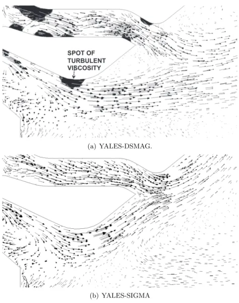
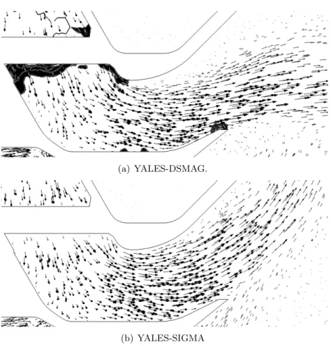
From tables 3.7 & 3.12 is evident that, for the LOTAR fixed swirler case, the AJ state is characterized by a lower swirl ratio (Sr 0.7) in the radial jet while the BB state is characterized by an higher swirl ratio (Sr 0.81) in the radial jet. This variation of the swirl ratio can be justified only by an effective geometry variation due to SGS modeling. Because of the eddy viscosity hypotheses, turbulent viscosity in AVBP and YALES2 is proportional to the strain rate tensor per the turbulent viscosity generated by the SGS model, see section 3.2.2. The level of strain rate inside the swirler is high at the solid boundaries, because of the no slip condition coupled with an insufficient wall resolution. The Dynamic Smagorinsky model generates high levels of turbulent viscosity at the solid boundary while the SIGMA model is built to generate low turbulent viscosity levels. The outcome is that the Dynamic Smagorinky simulations show multiple spots of high turbulent diffusion which damp the flow momentum and that are seen by the flow as obstacles, with the stream lines flowing around them. Even if the mesh is not modified, the flow sees a different section depending on the SGS model used. An example of how a spot of high turbulent diffusion can modify the flow is shown in Fig. A.1: the presence of this obstacle-like zone helps the jet to detach, while its absence make it stick to the wall1. In Fig. A.2 are shown the velocity vectors and the field of turbulent viscosity in the radial swirler for LES YALES-DSMAG and YALES-SIGMA.
These two phenomena, high turbulent diffusion and the modification of the effective geometry, have a deep impact in a particular zone: the radial swirler bowl. Here, at the exit of the vane passsages, all the jets coming from the swirler passages merge. In a distance of O(1mm), the velocity magnitude varies from 100[m/s] in the core of one jet, to zero, because of the solid boundary, and again to 100[m/s] because of the neighbouring jet, Fig. A.3. Note that, considering a boundary layer at a streamwise position x = 0.01[m] (the length of the swirler vane) and a freestream velocity U0 = 100[m/s], the boundary
1
It can be argued that the detachment dynamics of the central jet can be related to the swirl number (Eq.(2.2)) of the outermost axial jet, which is ≤ 0.43 for all the detached cases while it is ≥ 0.58 for all the attached ones. Chapter 4 shows how an attached central jet can be obtained with a swirl ≤ 0.43, and that its dynamics are not linked to the swirl number.
188 APPENDIX A. EFFECTS OF TURBULENT VISCOSITY ON LOTAR
(a) YALES-DSMAG.
(b) YALES-SIGMA
Figure A.1: Central jet detachment, (a) detached vs. (b) attached. Vector field is the mean flow velocity, the black spot of time averaged turbulent viscosity (corresponding to a µt/µ≥ 100) acts as an obstacle and induces the flow
separation.
layer thickness (the distance from the wall at which the mean flow speed reaches 99% the free stream speed, U0) is 0.4[mm]. Considering that the geometric length scales of the flow are of the same order of magnitude, it is now evident why numerous difficulties have been encountered during the simulation this particular area of the flow field.
Because of the large velocity gradient, numerical errors in this region can be large and affect the solution, for instance introducing an additional, un-physical, turbulence to the flow field. Turbulent viscosity generated by the SGS model interacts with the velocity field, causing a damping effect on the turbulence generated by the jet-to-jet interaction (natural or numerically generated), Fig. A.4. The overall effect is a modification of the mean velocity profile with a consequent variation of the swirl ratio of the jet depending on the turbulent viscosity level. The same phenomenon is happening in the outer and inner axial jets, where each jet is separated from its neighbour by a O(1mm) wall. While for
189
(a) YALES-DSMAG.
(b) YALES-SIGMA
Figure A.2: Turbulent viscosity and velocity vectors inside the radial swirler and inside the diffuser.
the outer axial jet a strong variation of the swirl number is experienced switching from Dynamic Smagorinsky to SIGMA, for the inner jet it is not and all simulations give a measured swirl in the inner axial jet of S 0.11 0.12.
190 APPENDIX A. EFFECTS OF TURBULENT VISCOSITY ON LOTAR
(a) YALES-DSMAG. (b) YALES-SIGMA
Figure A.3: Multiple jets in the LOTAR simulation. Turbulent over laminar viscosity field in the radial swirler vane, line corresponds to 50[m/s] velocity magnitude.
(a) YALES-DSMAG (b) YALES-SIGMA
Appendix B
Coflow effects on the LOTAR
adjustable swirler case
This appendix shows the effects of the coflow speed on the flow structures (and in general of the far field conditions) on the LOTAR adjustable swirler case of chapter 4. Its objective is to verify that the small velocity added in the coflow (Fig. 3.3) has a very limited effect on the results.
For this type of flow (a confined swirling jet) the jet dynamics are mainly governed by the swirler-diffuser geometry and the far field has only a secondary effect on the flow configuration. As shown in Vanierschot et al. [107] it is possible to achieve drastic change in the jet pattern (causing instantaneous transitions such as AJ-WJ or WJ-BB) by modifying the flow field at the injector nozzle and this way activating/deactivating the flow structures generated between the jet outer shear layer and the solid walls. Focusing on LES, this last simulation, named coflow, has the same characteristics of simulation high of table 4.1 but it has an higher coflow speed of 10[m/s] equivalent to 13% of the jet speed. Data are collected after a period of 50[ms], time needed by the coflow jet to reach and overtake the injector (0.37[m] downstream of the coflow B.C. shown in Fig. 3.3). As evident from Fig. B.1, the coflow speed has a reduced influence on the flow direction and the jet remains attached to the side walls of the injector (Fig. B.2) in the BB state. Despite the fact that the size of the recirculation zone (Fig. B.3) is smaller, the jet topology is unaltered as evident from the turbulence intensity and pressure fields (Fig. B.4). Finally, the whole flow field of LES high and coflow are compared in Fig. B.5.
192 APPENDIX B. COFLOW EFFECTS
Figure B.1: Flow field and velocity isoline (U = 20[m/s]) of simulations coflow. The jet opening half-angle is slightly smaller than LES high of table 4.5 (Fig. 4.12).
Figure B.2: Pressure field of the coflow LES studied here (legend is the same of Fig. 4.15d). A pressure gradient from the side-walls toward the core of the CTRZ is still present as in LES high of table 4.5.
193
Figure B.3: Comparison of the recirculation bubbles of LES high of table 4.5 and coflow studied here. Despite the reduction of the size of the CTRZ for LES coflow, the flow topology is unaltered with a CTRZ that is equally expanding in the radial and axial directions.
Figure B.4: Axial velocity RMS and pressure distribution measured along the centerline of the geometry. Results are plotted against normalized axial distance (X/R0) from the swirler ending plate for simulations high of table 4.5
194 APPENDIX B. COFLOW EFFECTS
Figure B.5: Far field of simulations high of table 4.5 and coflow. The higher coflow speed is evident from the instantaneous velocity magnitude field.
Appendix C
Effects of turbulence injection for
the ”axial” case of Delenback
This appendix shows the effect of turbulence injection for the ”axial” case of Dellenback experiment shown in Chapter 7. Turbulence is injected at the inlet of the domain (Fig. 7.1). The amount of turbulence necessary to match experimental data is dependent on the particular mesh and/or LES solver and settings used. For instance, a too coarse mesh or a too dissipative numerical scheme can nullify the effects of turbulence injection by damp-ing it just downstream the injection position. Therefore, this test is performed for one of the simulations/meshes of table 7.2 only and turbulence intensity is adjusted to match experimental data. The mesh chosen (numerical settings do not change for LES of table 7.2) is LES H3 and it is named here H3T J, where the subscript TJ stands for turbulence injection. Turbulence injected has an intensity T I = u0/U = 0.043 and a characteristic lenght scale of 10[mm] 15D1.
Results are shown in Fig. C.1 where the velocity profiles of LES H3T J are compared with the velocity profiles of LES H1, H2 and H3 of table 7.2 and experimental data at the 8 measurement planes of Fig. 7.2.
Fig. C.1 shows that the injection of turbulence allows to better match experimental data at plane 1 and at plane 4 (with the same accuracy of LES H1) without being particularly detrimental for the flow speed at the downstream planes. It is also verifies the assump-tion of secassump-tion 7.2.1, namely that results of LES H1 showed the best comparison with experimental data at plane 4 thanks to wall-generated numerical noise. This noise affects the growth rate of the shear layer instability, modifying the flow speed. Finally, Fig. C.2 shows how deep (comparing its negligible effects on the mean velocity profiles shown in Fig. C.1) is the influence of turbulence injection on RMS values.
196 APPENDIX C. EFFECTS OF TURBULENCE INJECTION 0 0,1 0,2 0,3 0,4 0,5 R/Rref 0 0,1 0,2 0,3 0,4 0,5 0,6 0,7 0,8 0,9 1 U/U ref EXP H1 H2 H3 H3_TJ
(a) Mean axial velocity profile at plane 2
0 0,1 0,2 0,3 0,4 0,5 0,6 0,7 0,8 0,9 1 R/R ref -0,1 0 0,1 0,2 0,3 0,4 0,5 0,6 0,7 0,8 0,9 1 1,1 U/U ref
(b) Mean axial velocity profile at plane 4
0 0,1 0,2 0,3 0,4 0,5 0,6 0,7 0,8 0,9 1 R/R ref -0,2 -0,1 0 0,1 0,2 0,3 0,4 0,5 0,6 0,7 0,8 0,9 1 1,1 U/U ref
(c) Mean axial velocity profile at plane 5
0 0,1 0,2 0,3 0,4 0,5 0,6 0,7 0,8 0,9 1 R/R ref -0,1 0 0,1 0,2 0,3 0,4 0,5 0,6 0,7 0,8 0,9 1 U/U ref
(d) Mean axial velocity profile at plane 6
0 0,1 0,2 0,3 0,4 0,5 0,6 0,7 0,8 0,9 1 R/R ref -0,1 0 0,1 0,2 0,3 0,4 0,5 0,6 0,7 0,8 0,9 1 U/U ref
(e) Mean axial velocity profile at plane 7
0 0,1 0,2 0,3 0,4 0,5 0,6 0,7 0,8 0,9 1 R/R ref 0 0,1 0,2 0,3 0,4 0,5 0,6 U/U ref
(f) Mean axial velocity profile at plane 8
0 0,1 0,2 0,3 0,4 0,5 0,6 0,7 0,8 0,9 1 R/R ref 0 0,1 0,2 0,3 0,4 U/U ref
(g) Mean axial velocity profile at plane 9
0 0,1 0,2 0,3 0,4 0,5 0,6 0,7 0,8 0,9 1 R/R ref 0 0,1 0,2 0,3 U/U ref
(h) Mean axial velocity profile at plane 10
Figure C.1: Mean axial velocity profiles at the measurement planes of Fig. 7.2 for simulations H1, H2, H3 of table 7.2 and LES H3T J (TJ stands for turbulence injection).
197 0 0,1 0,2 0,3 0,4 0,5 R/R ref 0 0,1 TI EXP H1 H2 H3 H3_TJ
(a) TI axial velocity at plane 2
0 0,1 0,2 0,3 0,4 0,5 0,6 0,7 0,8 0,9 1 R/R ref 0 0,1 0,2 TI
(b) TI axial profile at plane 4
0 0,1 0,2 0,3 0,4 0,5 0,6 0,7 0,8 0,9 1 R/R ref 0 0,1 0,2 TI
(c) TI axial profile at plane 5
0 0,1 0,2 0,3 0,4 0,5 0,6 0,7 0,8 0,9 1 R/R ref 0 0,1 0,2 TI
(d) TI axial profile at plane 6
0 0,1 0,2 0,3 0,4 0,5 0,6 0,7 0,8 0,9 1 R/R ref 0 0,1 0,2 TI
(e) TI axial profile at plane 7
0 0,1 0,2 0,3 0,4 0,5 0,6 0,7 0,8 0,9 1 R/R ref 0 0,1 0,2 TI
(f) TI axial profile at plane 8
0 0,1 0,2 0,3 0,4 0,5 0,6 0,7 0,8 0,9 1 R/R ref 0 0,1 0,2 TI
(g) TI axial profile at plane 9
0 0,1 0,2 0,3 0,4 0,5 0,6 0,7 0,8 0,9 1 R/R ref 0 0,1 TI
(h) TI axial profile at plane 10
Figure C.2: TI axial profiles (T I = uRM S
uref =
uRM S
8.92[m/s]) at the measurement planes of Fig. 7.2 for simulations H1,
Appendix D
Comparison of the flow states of
LOTAR and Vanierschot
In this appendix, the two flow topologies of LOTAR shown in chapters 3 and 4, the ”Axial Jet” (AJ) and the ”Blasted Breakdown jet”(BB), are compared with the same flow states of the experimental study of Vanierschot and Van Den Bulck [105]. The comparison is carried on in terms of pressure deficit and turbulence intensity.
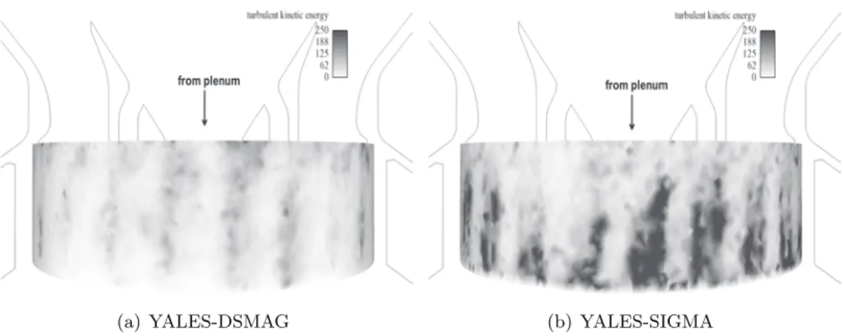
Fig. D.1 shows the ratio of the mean, axial, turbulent kinetic energy normalized by the jet kinetic energy U2 for the LOTAR and Vanierschot’s cases [105]. Despite the large geometric discrepancies between the two configurations, normalized turbulence levels are similar in both flows when the same flow state is compared.
Corcerning the pressure deficit (Eq.(2.9)), in both cases the BB state is characterized by a zero pressure deficit, while the AJ states is characterized by a PD 1.5 for Vanierschot’s case and PD 0.4 for LOTAR. Note that it was not possible to generate a graph similar to Fig. D.1 for the pressure deficit because of the lack of similar data for Vanierschot’s case.
Figure D.1: Comparison of LOTAR LES basic and high and experimental data (EXP) of Chapter 4 with Vanier-schot’s results [105] for the AJ and BB states. Normalization conditions for LOTAR are U = 61.17[m/s] and R0= 30[mm].
Bibliography
[1] Flying above the clouds. The Economist, 2011.
[2] 17th International Meshing Roundtable. Anisotropic Delaunay mesh adaptation for unsteady simulations, 1997.
[3] F. Alauzet, P.J. Frey, P.L. George, and B. Mohammadi. 3d transient fixed point mesh adaptation for time-dependent problems: Application to cfd simulations. Journal of Computational Physics, 222(2):592 – 623, 2007.
[4] Fr´ed´eric Alauzet and Pascal J. Frey. Estimateur d’erreur g´eom´etrique et m´etriques anisotropes pour l’adaptation de maillage. Partie I : aspects th´eoriques. Rapport de recherche RR-4759, INRIA, 2003.
[5] S. V. Apte, K. Mahesh, M. Gorokhovski, and P. Moin. Stochastic modeling of atomizing spray in a complex swirl injector using large eddy simulation. Proc. Combust. Inst., 32:2257–2266, 2009.
[6] AVBP. Avbp code: www.cerfacs.fr/cfd/avbp code.php and
www.cerfacs.fr/cfd/cfdpublications.html.
[7] D. Barre, M. Kraushaar, G. Staffelbach, V. Moureau, and L.Y.M. Gicquel. Com-pressible and incomCom-pressible les of a swirl experimental burner. In 3rd INCA Collo-quim, 2011.
[8] J. M. Beer and N. A. Chigier. Combustion aerodynamics. Krieger, Malabar, Florida, 1983.
[9] T. Brooke Benjamin. Theory of the vortex breakdown phenomenon. Journal of Fluid Mechanics, 14:593–629, 11 1962.
[10] P. Billant, J.-M. Chomaz, and P. Huerre. Experimental study of vortex breakdown in swirling jets. J. Fluid Mech., 376:183–219, 1998.
[11] M. Boileau, S. Pascaud, E. Riber, B. Cuenot, L.Y.M. Gicquel, T. Poinsot, and M. Cazalens. Investigation of two-fluid methods for Large Eddy Simulation of spray combustion in Gas Turbines. Flow, Turb. and Combustion, 80(3):291–321, 2008. [12] S. T. Bose, P. Moin, and D. You. Grid-independent large-eddy simulation using
explicit filtering. Phys. Fluids, 22(10):105103, October 2010. 199
200 BIBLIOGRAPHY [13] John J. Cassidy and Henry T. Falvey. Observations of unsteady flow arising after
vortex breakdown. Journal of Fluid Mechanics, 41(04):727–736, 1970.
[14] Jean Cea. Approximation variationnelle des probl`emes aux limites. PhD thesis, 1964.
[15] D. R. Chapman and G. D. Kuhn. The limiting behaviour of turbulence near a wall. J. Fluid Mech., 170:265–292, 1986.
[16] Fotini Katopodes Chow and Parviz Moin. A further study of numerical errors in large-eddy simulations. Journal of Computational Physics, 184(2):366 – 380, 2003. [17] P. Dellenback, D. Metzger, and G. Neitzel. Measurement in turbulent swirling flows
through an abrupt axisymmetric expansion. AIAA Journal, 13(4):669–681, 1988. [18] Cecile Dobrzynski. Adaptation de Maillage anisotrope 3D et application a
l’aero-thermique des batiments. PhD thesis, Universite Pierre et Marie Curie, Paris VI, 2005.
[19] Cecile Dobrzynski. MMG3D manual. INRIA, 2010.
[20] J Dombard, T Poinsot, V Moureau, N Savary, G Staffelbach, and V Bodoc. Exper-imental and numerical study of the influence of small geometrical modifications on the dynamics of swirling flows. In CTR, Proceedings of the Summer Program 2012. [21] E.Bank. Mesh smoothing using a posteriori error estimates. SIAM Journal on
Numerical Analysis, Vol. 34(No. 3):pp. 979–997, Jun., 1997.
[22] M.P. Escudier and J.J. Keller. Vortex breakdown: a two stage transition. Technical report, Brown Boveri Research center Baden (Switzerland), 1983.
[23] J. H. Faler and S. Leibovich. Disrupted states of vortex flow and vortex breakdown. Phys. Fluids, 20:1395–1400, 1977.
[24] L. Freitag, M. Jones, and P. Plassmann. An efficient parallel algorithm for mesh smoothing. In Proceedings of the 4th International Meshing Roundtable, Sandia National Laboratories, 1995.
[25] P.J. Frey and F. Alauzet. Anisotropic mesh adaptation for cfd computations. Com-puter Methods in Applied Mechanics and Engineering, 194(48–49):5068 – 5082, 2005. [26] Isaac Fried. Condition of finite element matrices generated from nonuniform meshes.
1972.
[27] J. Frøhlich, C. P. Mellen, W. Rodi, L. Temmerman, and M. A. Leschziner. Highly re-solved large-eddy simulation of separated flow in a channel with streamwise periodic constrictions. J. Fluid Mech., 526:19–66, 2005.
[28] M. Garc´ıa-Villalba, J. Fr¨ohlich, and W. Rodi. Identification and analysis of coherent structures in the near field of a turbulent unconfined annular swirling jet using large eddy simulation. Phys. Fluids, 18, 2006.
BIBLIOGRAPHY 201 [29] M. Germano, U. Piomelli, P. Moin, and W. Cabot. A dynamic subgrid-scale eddy
viscosity model. Phys. Fluids, 3(7):1760–1765, 1991.
[30] B. J. Geurts and J.Fr¨ohlich. A framework for predicting accuracy limitations in large-eddy simulation. Phys. Fluids, 14, 2002.
[31] S. Ghosal. An analysis of numerical errors in large eddy simulations of turbulence. J. Comput. Phys., 125:187 – 206, 1996.
[32] A. K. Gupta, D. G. Lilley, and N. Syred. Swirl flows. Abacus Press, 1984.
[33] Wagdi G. Habashi, Julien Dompierrea, Yves Bourgaulta, Djaffar Ait-Ali-Yahiaa, Michel Fortin, and Marie-Gabrielle Vallet. Anisotropic mesh adaptation: towards user-independent, mesh-independent and solver-independent cfd. part i: general principles. Int. J. Numer. Meth. Fluids, 32:725–744, 2000.
[34] M. G. Hall. Vortex breakdown. Ann. Rev. Fluid Mech, 4:195–217, 1972.
[35] M.G. Hall. The structure of concentrated vortex cores. Progress in Aerospace Sci-ences, 7(53-110), 1966.
[36] G. Hannebique, P. Sierra, E. Riber, and B. Cuenot. Large Eddy Simulation of reactive two-phase flow in aeronautical multipoint burner. In 7th Mediterranean Combustion Symposium - September 11-15, Chia Laguna, Cagliari, Sardinia, Italy, 2011.
[37] Claudia Hertel and Jochen Fr¨ohlich. Error reduction in les via adaptive moving grids. In Maria Vittoria Salvetti, Bernard Geurts, Johan Meyers, and Pierre Sagaut, edi-tors, Quality and Reliability of Large-Eddy Simulations II, volume 16 of ERCOFTAC Series, pages 309–318. Springer Netherlands, 2011.
[38] J. Hoffman. computation of mean drag for bluff body problems using adaptive DNS/LES. SIAM Journal on Scientific Computing, 27(1):184–207, 2005.
[39] J. Hoffman and C. Johnson. A new approach to computational turbulence modeling. Computer Methods in Applied Mechanics and Engineering, 195(23–24):2865 – 2880, 2006.
[40] P. G. Huang and G. N. Coleman. Van driest transformation and compressible wall-bounded flows. AIAA Journal, 32(10):2110–2113, 1994.
[41] Weizhang Huang. Variational mesh adaptation: Isotropy and equidistribution. Jour-nal of ComputatioJour-nal Physics, (174):903–924, 2001.
[42] Y. Huang, S. Wang, and V. Yang. Systematic analysis of lean-premixed swirl-stabilized combustion. AIAA Journal, 44(724-740), 2006.
[43] Ying Huang and Vigor Yang. Dynamics and stability of lean-premixed swirl-stabilized combustion. Progress in Energy and Combustion Science, 35(4):293 – 364, 2009.
202 BIBLIOGRAPHY [44] J. C. R. Hunt, A. A. Wray, and P. Moin. Eddies, streams, and convergence zones in turbulent flows. In Proc. of the Summer Program, pages 193–208. Center for Turbulence Research, NASA Ames/Stanford Univ., 1988.
[45] A. K. Aziz I. Babuska. On the angle condition in the finite element method. SIAM J. NUMER. ANAL., 13(2), April 1976.
[46] A.K. Chesters J. Chedaille, W. Leuckel. Aerodynamic studies carried out on tur-bulent jets by the international flame research. Journal of the institute of Fuel, 39(311):506–521, 1966.
[47] F. Jaegle. LES of two-phase flow in aero-engines. PhD thesis, Universit´e de Toulouse - Ecole doctorale MEGeP, CERFACS - CFD Team, Toulouse, December 2009. [48] F. Jaegle, J.-M. Senoner, M. Garcia, F. Bismes, R. Lecourt, B. Cuenot, and
T. Poinsot. Lagrangian and eulerian simulations of evaporating fuel spray in an aeronautical multipoint injector. Proc. Combust. Inst., 33:2099–2107, 2011.
[49] J. Jimenez. On why dynamic subgrid-scale models work. Technical report, 1995. [50] J. Jim´enez. Turbulence and vortex dynamics. Technical Report Ecole Polytechnique,
2004.
[51] J. Jim´enez and R. D. Moser. Large-eddy simulations: where are we and what can we expect? AIAA Journal, 23(4):605–612, April 2000.
[52] Won-Wook Kim and Saadat Syed. Large-eddy simulation needs for gas-turbine combustor design. (0331), 2004.
[53] Markus Klein, Johan Meyers, and Bernard J. Geurts. Assessment of les quality mea-sures using the error landscape approach. In Johan Meyers, Bernard J. Geurts, and Pierre Sagaut, editors, Quality and Reliability of Large-Eddy Simulations, volume 12 of ERCOFTAC Series, pages 131–142. Springer Netherlands, 2008.
[54] A. N. Kolmogorov. The local structure of turbulence in incompressible viscous fluid for very large reynolds numbers. C. R. Acad. Sci., USSR, 30:301, 1941.
[55] Matthias Krausaar. Application of the compressible and low-Mach number ap-proaches to Large-Eddy Simulation of turbulent flows in aero-engines. PhD thesis, CERFACS, 2011.
[56] A. G. Kravchenko and P. Moin. On the effect of numerical errors in large eddy simulations of turbulent flows. J. Comput. Phys., 131(2):310–322, March 1997. [57] Y.A. Kuznetsov. Elements of Applied Bifurcation Theory. Springer, 1998.
[58] E. Lamballais and J.P. Bonnet. DNS/LES data processing and its relation with experiment, February 2003. ISSN 0377-8312 VKI Lectures Series 2003-03 ”Post-processing of experimental and numerical data ISSN 0377-8312.
BIBLIOGRAPHY 203 [59] N. C. Lambourne and D. W. Bryer. The bursting of leading-edge vortices: Some observations and discussions of the phenomenon. Technical Report R. & M, Aero-nautical Research Council (G.B.), 1961.
[60] H. Liang and T. Maxworthy. An experimental investigation of swirling jets. Journal of Fluid Mechanics, 525:115–159, 1 2005.
[61] T. Loiseleux, J. M. Chomaz, and P. Huerre. The effect of swirl on jets and wakes: Linear instability of the rankine vortex with axial flow. Physics of Fluids, 10(5):1120– 1134, 1998.
[62] Adrien Loseille and Fr´ed´eric Alauzet. Continuous Mesh Model and Well-Posed Con-tinuous Interpolation Error Estimation, 2009. Rapport de recherche INRIA.
[63] Adrien Loseille, Alain Dervieux, Pascal Frey, and Frederic Alauzet. Achievement of global second-order mesh convergence for discontinuous flows with adapted unstruc-tured meshes. In 18th AIAA computatonal Fluid Dynamics Conference, 2007. [64] O. Lucca-Negro and T. O’Doherty. Vortex breakdown: a review. Prog. Energy
Comb. Sci., 27:431–481, 2001.
[65] D. Lucor, J. Meyers, and P. Sagaut. Sensitivity analysis of large-eddy simulations to subgrid-scale-model parametric uncertainty using polynomial chaos. Journal of Fluid Mechanics, 585:255–279, 2007.
[66] T. S. Lund. The use of explicit filters in large eddy simulation. Computers and Mathematics with Applications, 46(4):603–616, August 2003.
[67] K. Mahesh, G. Constantinescu, and P. Moin. A numerical method for large-eddy simulation in complex geometries. J. Comput. Phys., 197(1):215–240, 2004. [68] C. Martin, L. Benoit, Y. Sommerer, F. Nicoud, and T. Poinsot. Les and acoustic
analysis of combustion instability in a staged turbulent swirled combustor. AIAA Journal, 44(4):741–750, 2006.
[69] Carl Ollivier-Gooch M.Batford, Lori A. Freitag. Computational study of the effect of unstructured mesh quality on solution efficiency.
[70] C. Meneveau and J. Katz. Scale-invariance and turbulence models for large eddy simulation. Ann. Rev. Fluid Mech, 32:1–32, 2000.
[71] J. Meyers, B.J. Geurts, and P. Sagaut. A computational error-assessment of central finite-volume discretizations in large-eddy simulation using a smagorinsky model. Journal of Computational Physics, 227(1):156 – 173, 2007.
[72] Johan Meyers and Pierre Sagaut. Is plane-channel flow a friendly case for the testing of large-eddy simulation subgrid-scale models? Physics of Fluids, 19(4):048105, 2007.
[73] R. Mittal and P. Moin. Suitability of upwind-biased finite difference schemes for large-eddy simulation of turbulent flows. AIAA Journal, 35:1415–1417, 1997.
204 BIBLIOGRAPHY [74] P. Moin and S. V. Apte. Large-eddy simulation of realistic gas turbine combustors.
AIAA Journal, 44(4):698–708, 2006.
[75] St`ephane Moreau. Private conversation, September 2013.
[76] V. Moureau, P. Domingo, and L. Vervisch. From large-eddy simulation to direct numerical simulation of a lean premixed swirl flame: Filtered laminar flame-pdf modeling. Combust. Flame, in press, 2011.
[77] V. Moureau, G. Lartigue, Y. Sommerer, C. Angelberger, O. Colin, and T. Poinsot. Numerical methods for unsteady compressible multi-component reacting flows on fixed and moving grids. J. Comput. Phys., 202(2):710–736, 2005.
[78] JM Beer N Syred. Vortex core precession in high swirl flows. In The second Interna-tional JSME Symposium on Fluid Machinery and Fluidics, Tokyo, volume 2, pages 111–120. JSME, 1972.
[79] F. Nicoud and F. Ducros. Subgrid-scale stress modelling based on the square of the velocity gradient. Flow, Turb. and Combustion, 62(3):183–200, 1999.
[80] Franck Nicoud, Hubert Baya Toda, Olivier Cabrit, Sanjeeb Bose, and Jungil Lee. Using singular values to build a subgrid-scale model for large eddy simulations. Phys. Fluids, 23, 2011.
[81] K Oberleithner, S Terhaar, L Rukes, and C O Paschereit. Why non-uniform density suppresses the precessing vortex core. In Proceedings of ASME Turbo Expo 2013. [82] F. Bismes-F. Simon P. Gajan, J. Apeloig. Kiai deliverable d2.3.1: Experimental
characterization of the injector. 2011.
[83] P. Palies. Dynamique et instabilies de combustion de flammes swirlees. Phd thesis, Ecole Centrale Paris, 2010.
[84] Noma Park and Krishnan Mahesh. Analysis of numerical errors in large eddy simu-lation using statistical closure theory. Journal of Computational Physics, 222(1):194 – 216, 2007.
[85] P.; Reynolds W.C. Pauley, L.L.; Moin. The structure of two-dimensional separation. J. Fluid Mech., 1990.
[86] U. Piomelli, W. H. Cabot, P. Moin, and S. Lee. Subgrid-scale backscatter in turbu-lent and transitional flows. Phys. FluidsA, 3(7):1766–1771, July 1991.
[87] T. Poinsot and S. Lele. Boundary conditions for direct simulations of compressible viscous flows. J. Comput. Phys., 101(1):104–129, 1992.
[88] T. Poinsot and D. Veynante. Theoretical and Numerical Combustion. R.T. Edwards, 2nd edition, 2005.
BIBLIOGRAPHY 205 [90] S. B. Pope. Ten questions concerning the large-eddy simulation of turbulent flows.
New Journal of Physics, 6:35, 2004.
[91] S. Roux, G. Lartigue, T. Poinsot, U. Meier, and C. B´erat. Studies of mean and unsteady flow in a swirled combustor using experiments, acoustic analysis and large eddy simulations. Combust. Flame, 141:40–54, 2005.
[92] M. Rudgyard. Integrated preprocessing tools for unstructured parallel cfd applica-tions. Technical Report TR/CFD/95/08, CERFACS, 1995.
[93] M. Rudgyard, T. Schoenfeld, R. Struijs, G. Audemar, and P. Leyland. A modu-lar approach for computational fluid dynamics. Technical Report TR/CFD/95/07, CERFACS, 1995.
[94] P. Sagaut. Large eddy simulation for incompressible flows. Springer, 2002.
[95] M. Sanjos´e, E. Riber, L. Gicquel, B. Cuenot, and T. Poinsot. Large Eddy Simulation of a two-phase reacting flow in an experimental burner. In ERCOFTAC Workshop - DLES7, pages 251–263, Trieste, Italy, September 2008.
[96] T. Sarpkaya. On stationary and travelling vortex breakdowns. J. Fluid Mech., 45:545–559, 1971.
[97] A. Scotti, C. Meneveau, and M. Fatica. Generalized smagorinski model for anisotropic grids. Phys. Fluids, 9(6):1856–1858, 1997.
[98] A. Scotti, C. Meneveau, and D. K. Lilly. Generalized smagorinski model for anisotropic grids. Phys. Fluids, 5(9):2306–2308, 1993.
[99] L. Selle, L. Benoit, T. Poinsot, F. Nicoud, and W. Krebs. Joint use of compressible large-eddy simulation and helmoltz solvers for the analysis of rotating modes in an industrial swirled burner. Combust. Flame, 145(1-2):194–205, 2006.
[100] L. Selle, G. Lartigue, T. Poinsot, R. Koch, K.-U. Schildmacher, W. Krebs, B. Prade, P. Kaufmann, and D. Veynante. Compressible large-eddy simulation of turbu-lent combustion in complex geometry on unstructured meshes. Combust. Flame, 137(4):489–505, 2004.
[101] Jean-Mathieu Senoner. Simulation aux Grandes ´Echelles de l’´ecoulement diphasique dans un brˆuleur a´eronautique par une approche Euler-Lagrange. PhD thesis, CER-FACS, 2010.
[102] N. Syred. A review of oscillation mechanims and the role of the precessing vortex core in swirl combustion systems. Prog. Energy Comb. Sci., 32(2):93–161, 2006. [103] L. Thobois, G. Rymer, and T. Souleres. Large-eddy simulation in IC engine
geome-tries. SAE, (2004-01-1854), 2004.
[104] L. Thobois, G. Rymer, T. Souleres, T. Poinsot, and B. Van den Heuvel. Large-eddy simulation for the prediction of aerodynamics in IC engine. Int. J. Vehicle Des., 39(4):368–382, 2005.
206 BIBLIOGRAPHY [105] M. Vanierschot and E. Van den Bulck. Hysteresis in flow patterns in annular swirling
jets. Experimental Thermal and Fluid Science, 31(6):513 – 524, 2007.
[106] M. Vanierschot and E. Van den Bulck. Influence of the nozzle geometry on the hysteresis of annular swirling jets. Combustion Science and Technology, 179(8):1451– 1466, 2007.
[107] M. Vanierschot, T. Persoons, and E. Van den Bulck. A new method for annular jet control based on cross-flow injection. Physics of Fluids, 21(2):25103–25112, 2009. [108] M. Vanierschot and E. Van den Bulck. Computation of a drastic flow pattern change
in an annular swirling jet caused by a small decrease in inlet swirl. International Journal for Numerical Methods in Fluids, 59(5):577–592, 2009.
[109] Shanwu Wang, Shih-Yang Hsieh, and Vigor Yang. Unsteady flow evolution in swirl injector with radial entry. i. stationary conditions. Physics of Fluids, 17(4):045106, 2005.
[110] Shanwu Wang and Vigor Yang. Unsteady flow evolution in swirl injectors with radial entry. ii. external excitations. Physics of Fluids, 17(4):045107, 2005.
[111] Shanwu Wang, Vigor Yang, George Hsiao, Shih-Yang Hsieh, and Hukam C. Mongia. Large-eddy simulations of gas-turbine swirl injector flow dynamics. J. Fluid Mech., 583:99–122, 2007.
[112] R. Wille and H. Fernholz. Report on the first european mechanics colloquium, on the coanda effect. Journal of Fluid Mechanics, 23(04):801–819, 1965.
Appendix E
Paper accepted for publication
(October 2013) in ”Computers
and Fluids”.
LES of bifurcation and hysteresis in confined annular
swirling flows
Mario Falese1
Centre Europeen de Recherche et de Formation Avancee en Calcul Scientifique (CERFACS), 31057 Toulouse, France.
L.Y.M. Gicquel
Centre Europeen de Recherche et de Formation Avancee en Calcul Scientifique (CERFACS), 31057 Toulouse, France.
Thierry Poinsot
Institut de Mecanique des Fluides de Toulouse (IMFT), 31100 Toulouse, France.
Abstract
This paper presents a LES based study of two swirling confined jet config-urations corresponding to an aeronautical injection system. The objectives are to demonstrate that LES codes become sensitive to numerical param-eters (grid, SGS model) in such cases and that this is due to the fact that these ows are close to bifurcating conditions because of the presence of swirl and confinement walls. To demonstrate this, in the first configuration ('full swirler'), the swirler/plenum ensemble is computed while only the swirler without plenum is computed in the second ('adjustable swirler'): this simpli-fication allows to vary swirl continuously and explore bifurcation diagrams
1Corresponding author, falese@cerfacs.fr, tel. +330561193109.
where the control parameter is the mean swirl number. These numerical results are compared to a similar study performed experimentally by Vanier-schot and Van Den Bulck [1]. They confirm that certain confined swirling ows are intrinsically submitted to bifurcations. In the context of LES this leads to a large sensitivity of the simulation results to numerical parameters, a property which is not observed in most other non swirling or non confined situations.
Keywords: LES, swirl ows, bifurcation, hysteresis, numerical simulations, swirling jets, aeronautical injector
Nomenclature
D0 = jet characteristic diameter [m]
R0 = jet characteristic radius [m]
U0 = jet characteristic speed [m=s]
x, X = axial position [m] r, R = radial position [m] S = swirl number [ ] ua = axial velocity [m=s] uθ = tangential velocity [m=s] ur = radial velocity [m=s] U = jet velocity [m=s] = density [kg=m3] = grid size [m] T = temperature [K] P = pressure [kg=s2=m]
Patm = atmospheric pressure [kg=s2=m]
PD = normalized subpressure [ ]
y+ = nondimensional wall distance [ ]
P ope = Pope criterion [2] [ ]
kres = resolved, turbulent kinetic energy [m2=s2]
ksgs = SGS, turbulent kinetic energy [m2=s2]
t = turbulent viscosity [m2=s] Cm = SGS model constant [ ] CM = constant [ ] ~ u = filtered velocity [m=s] Dm(~u) = di erential operator [1=s] 3
1. Introduction
The objectives of this work are (1) to study bifurcation in confined swirling ows, typically swirlers used in combustion system, (2) to indicate specific aspects of LES methods to which careful attention must be paid for a suc-cessful simulation of an industrial swirling ow. Swirling jets are essential elements of many combustion chambers and lead to complex ows which control the fuel atomization, the shape of the recirculating zone produced in front of the swirler and ultimately a large part of the engine performances. Experimentalists know that bifurcation is a common feature in many swirling ows where multiple instabilities take place [3]. The most common of them is vortex breakdown [4, 5], which occurs when reverse ow takes place along the jet axis [6] because of the adverse pressure gradient induced by the con-servation of circulation and the jet expansion [4], as first proposed by Hall [7]. Seven di erent types of vortex breakdown have been identified depending on the swirl and Reynolds number [3] but there are numerous parameters ranges for which "two forms (or more) can exist and transform spontaneously into each other" [5]. Swirl intensity is one of the parameters controlling transition between ow states and its e ects will be analyzed here using LES, focus-ing the investigation on an aeronautical swirl injector. Two geometries are analyzed in this paper; in the first, named full swirler, the plenum (located upstream of the injector) and the swirler passages are included in the simu-lation domain (Fig. C.1). Results of the full swirler case show that LES can bifurcate depending on the grid resolution inside the radial swirler, under
the same in ow conditions. This property is observed exactly in the same manner for the two LES codes used here: AVBP [8, 9] & YALES2 [10] (a compressible and an incompressible LES solver respectively).
In the second geometry, named adjustable swirler (Fig. C.1), the sim-ulation domain, extracted from the full geometry of the full swirler case, starts downstream of the swirler vanes. The three counter-rotating swirlers, which together form the swirl injector, are replaced by a set of boundary conditions (B.C.s) in order to vary the swirl intensity as desired. This mod-ification allows to transform the original, swirl injector into an adjustable swirl device which can be used to change swirl over a wide range and to ex-plore the resulting ow topologies. The jet states generated in the adjustable swirler case show common, peculiar, properties with the experimental results of Vanierschot and Van Den Bulck [1]. Even if the exact limits of the di er-ent states and the hysteresis patterns di er (as a consequence of the di erer-ent geometries), both the present LES of an aeronautical swirler and the simpler configuration of Vanierschot et al. [1], exhibit similar bifurcations controlled by the swirl level and induced by the presence of confinement walls. This suggests that LES of confined swirling ows can be di cult because of their natural sensitivity to small swirl level variations: in the real world, this sen-sitivity leads to bifurcations and hysteresis mechanisms; in LES, it explains why simulation results of swirling ows are very sensitive to small details of the numerical setup (mesh, SGS model, boundary conditions) and re-quire much more attention. Section 2 first recalls evidences of bifurcation in
swirling ows obtained experimentally and presents a jet states classification based on ow properties. Section 3 describes the swirler investigated using LES here in the full swirler case and presents the e ects of bifurcation ob-served for this ow. The source of these bifurcations is identified in section 4, where the adjustable swirler is computed and a bifurcation diagram de-pending on the swirl number is constructed. Results of section 4 shows that LES is sensitive to numerical parameters in the full swirler case because the jet has a swirl number corresponding to an hysteresis zone, which is captured in the adjustable swirler LES.
2. Bifurcation in con ned swirling flows: experimental evidence. This section discusses ow states which can appear in confined swirling ows because of the proximity of solid boundaries. Above a critical swirl strength, confinement walls alter the expansion angle of the jet, which can attach to the sidewalls and behave like a radial jet, a phenomenon similar to the Coanda e ect [12]. The critical swirl number at which this transition takes place is dependent on the nozzle geometry as several phenomena such as separation of the jet, Coanda e ect and jet expansion angle all play a role. In Chedaille et al. [13], three di erent swirling jet configurations ap-pear depending on the nozzle opening angle or on the expansion rate of the divergent nozzle. Similar jet configurations and recirculation zones are re-ported by Beer and Chigier [14], in a qualitative manner and more recently by Vanierschot and Van Den Bulck [1]. The experiment of Vanierschot et
al. [1], provides a quantitative analysis of a ow with variable swirl and it will be used as a reference example to classify ow states. Vanierschot et al. [1], investigate the in uence of swirl on an annular jet with a stepped-conical expansion (Re = 11000), identifying four, distinct ow states.
The first two states identified by Vanierschot et al. [1], are named here, "Un-broken axial jet" (UJ) and "free Axial Jet" (AJ) (Fig.C.2). UJ states
are obtained when S < 0:4 while AJ states appear for S 0:4, where the
swirl number S is defined by: S =
R
A uauθrdA
R0RA uauadA
: (1)
At S = 0:4, vortex breakdown takes place in this configuration. The tran-sition between the "Axial Jet" and the "Weak axial Jet" (WJ), as named here, and the transition between the WJ and the "Blasted Breakdown jet" (BB), as named here, take place as follows (Fig. C.3).
First, increasing the swirl number up, from state AJ, to the second crit-ical threshold of S = 0:6, the ow bifurcates to the WJ state. The AJ-WJ transition is the result of the attachment of the jet to the side walls of the nozzle (Fig.C.2) which causes a widening of the expansion angle of the jet and the creation of a "corner recirculation zone" between the jet and the dif-fuser walls [15]. This bifurcation is characterized by an abrupt expansion of the Central Toroidal Recirculation Zone (CTRZ) which doubles its diameter (Fig. C.2). At the same time, the azimuthal velocity, the sub-pressure in the CTRZ and turbulence levels, decrease. Because of hysteresis, the WJ state
![Figure 9.8: Velocity profiles of LES of table 3.13 and LES ADAPTED of table 9.1. 15mm plane, R 0 = 30[mm].](https://thumb-eu.123doks.com/thumbv2/123doknet/3517029.102865/10.918.214.755.109.1089/figure-velocity-profiles-les-table-adapted-table-plane.webp)
![Figure 9.9: Velocity profiles of LES of table 3.13 and LES ADAPTED of table 9.1. 30mm plane, R 0 = 30[mm].](https://thumb-eu.123doks.com/thumbv2/123doknet/3517029.102865/11.918.158.702.101.1102/figure-velocity-profiles-les-table-adapted-table-plane.webp)
![Figure B.1: Flow field and velocity isoline (U = 20[m/s]) of simulations coflow. The jet opening half-angle is slightly smaller than LES high of table 4.5 (Fig](https://thumb-eu.123doks.com/thumbv2/123doknet/3517029.102865/24.918.191.789.111.452/figure-velocity-isoline-simulations-coflow-opening-slightly-smaller.webp)