H/V ratio: a tool for site effects evaluation. Results from 1-D noise simulations

GJI

Seismology

H/V ratio: a tool for site effects evaluation. Results from 1-D

noise simulations

Sylvette Bonnefoy-Claudet,

C´ecile Cornou,

Pierre-Yves Bard,

Fabrice Cotton,

Peter Moczo,

Jozef Kristek

and Donat F¨ah

1_{Laboratoire de G´eophysique Interne et de Tectonophysique, University Joseph Fourier, Grenoble, France} 2_{ETH Hoenggerberg, Institute of Geophysics, Zurich, Switzerland}

3_{Laboratoire Central des Ponts-et-Chauss´ees, Paris, France}

4_{Department of Physics of the Earth and Planets, Comenius University, Bratislava, Slovakia} 5_{Geophysical Institute, Slovak Academy of Sciences, Bratislava, Slovakia}

Accepted 2006 July 27. Received 2006 July 21; in original form 2005 July 29

S U M M A R Y

Ambient vibration techniques such as the H/V method may have the potential to significantly contribute to site effect evaluation, particularly in urban areas. Previous studies interpret the so-called Nakamura’s technique in relation to the ellipticity ratio of Rayleigh waves, which, for a high enough impedance contrast, exhibits a pronounced peak close to the fundamental S-wave resonance frequency. Within the European SESAME project (Site EffectS assessment using AMbient Excitations) this interpretation has been tested through noise numerical simulation under well-controlled conditions in terms of source type and distribution and propagation structure. We will present simulations for a simple realistic site (one sedimentary layer over bedrock) characterized by a rather high impedance contrast and low quality factor. Careful H/V and array analysis on these noise synthetics allow an in-depth investigation of the link between H/V ratio peaks and the noise wavefield composition for the soil model considered here: (1) when sources are near (4 to 50 times the layer thickness) and surficial, H/V curves exhibit one single peak, while the array analysis shows that the wavefield is dominated by Rayleigh waves; (2) when sources are distant (more than 50 times the layer thickness) and located inside the sedimentary layer, two peaks show up on the H/V curve, while the array analysis indicates both Rayleigh waves and strong S head waves; the first peak is due to both fundamental Rayleigh waves and resonance of head S waves, the second is only due to the resonance of head S waves; (3) when sources are deep (located inside the bedrock), whatever their distance, H/V ratio exhibit peaks at the fundamental and harmonic resonance frequencies, while array analyses indicate only non-dispersive body waves; the H/V is thus simply due to multiple reflections of S waves within the layer. Therefore, considering that experimental H/V ratio (i.e. derived from actual noise measured in the field) exhibit in most cases only one peak, we conclude that H/V ratio is (1) mainly controlled by local surface sources, (2) mainly due to the ellipticity of the fundamental Rayleigh waves. Then the amplitude of H/V peak is not able to give a good estimate of site amplification factor.

Key words: H/V, microtremor, seismic array, seismic modelling, seismic noise, site effects.

1 I N T R O D U C T I O N

The H/V spectral ratio (i.e. the ratio between the Fourier ampli-tude spectra of the horizontal and the vertical component of

mi-∗_{Corresponding author: FMFI—Comenius University, Mlynska dolina F1,}

84248 Bratislava, Slovakia. E-mail: bonnefoy@fmph.uniba.sk.

crotremors) was first introduced by Nogoshi & Igarashi (1971), and widespread by Nakamura (1989, 1996, 2000). These authors have pointed out the correlation between the H/V peak frequency and the fundamental resonance frequency of the site, and they proposed to use the H/V technique as an indicator of the underground struc-ture feastruc-tures. Since then, a large number of experiments (Lermo & Chavez-Garcia 1993; Gitterman et al. 1996; Seekins et al. 1996; F¨ah 1997) have shown that the H/V procedure can be successful applied for identifying the fundamental resonance frequency of sedimentary

deposits. These observations were supported by several theoretical 1-D investigations (Field & Jacob 1993; Lachet & Bard 1994; Lermo & Chavez-Garcia 1994; Wakamatsu & Yasui 1996; Tokeshi & Sugimura 1998), that have shown that noise synthetics computed using randomly distributed, near surface sources lead to H/V ratios sharply peaked around the fundamental S-wave frequency, when the surface layer exhibits a sharp impedance contrast with the un-derlying stiffer formations. However, some discussions are still under way about the applicability of this technique to evaluating the site amplification (Bard 1998; Bour et al. 1998; Mucciarelli 1998; Al Yuncha & Luzon 2000; Maresca et al. 2003; Rodriguez & Midorikawa 2003). If the shape of the H/V curves is controlled by the S-wave resonance within the sediments Nakamura (1989, 2000), then both H/V peak frequency and amplitude may be straightforward related to the soil transfer function (in term of fundamental reso-nance frequency and site amplification factor). On the other hand, if the shape of the H/V curves is controlled by the polarization of fundamental Rayleigh waves (Lachet & Bard 1994; Kudo 1995; Bard 1998; Konno & Ohmachi 1998; F¨ah et al. 2001), then only an indirect correlation between the H/V peak amplitude and the site amplification may exist.

In order to better understand the noise wavefield characteristics and its subsequent ability to provide significant information about the site conditions, we have simulated for a well-known 1-D struc-ture (a sedimentary layer overlaying a half-space) noise generated by randomly distributed sources. Using different sources having dif-ferent depths and spatial location, we define the appropriate noise sources characteristics in order to get a good representation of the actual noise in terms of H/V and measured dispersion curves through array techniques. Then, the investigation of the noise wavefield com-position (body and/or surface waves) using array processing allows us to draw conclusion about the composition of noise wavefield at H/V peak frequencies.

2 N O I S E D AT A S E T S 2.1 Soil model

We consider a simple physical model representative of a soft site. It is composed of one homogeneous layer over a half-space, there-after called M2 model. This model is characterized by its thickness,

P- and S-wave velocities, mass density, and P- and S-wave quality

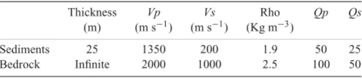
factors (Table 1). The values for the attenuation have been selected to model values typically observed or considered for sedimentary deposits (Hauksson et al. 1987; Fukushima et al. 1992; Wang et al. 1994; Jongmans et al. 1998; Di Giulio et al. 2003). The physi-cal characteristics of the M2 model have been chosen in order to illustrate the properties of a high impedance contrast (about 6.5) be-tween the sedimentary layer and the bedrock, for which it is known that the ellipticity of the fundamental mode of Rayleigh waves is very close to the S-wave resonance frequency of the site (Tokimatsu 1997; Konno & Ohmachi 1998; Malischewsky & Scherbaum 2004) as indicated in Fig. 1.

Table 1. Physical parameters for the M2 model (one layer over a half-space).

Thickness Vp Vs Rho Qp Qs

(m) (m s−1) (m s−1) (Kg m−3)

Sediments 25 1350 200 1.9 50 25

Bedrock Infinite 2000 1000 2.5 100 50

Figure 1. 1-D transfer function for vertically incident SH waves (plain line),

ellipticity of the fundamental mode (dashed line) and the first mode (dashed-dot line) of Rayleigh waves for the M2 model.

2.2 Sources and receivers configuration

The seismic ambient noise is the generic term used to denote ambient vibrations of the ground caused by sources such as tide, water waves striking the coast, turbulent wind, effects of wind on trees or build-ings, industrial machinery, cars and trains, or human footsteps, etc. The seismic ambient noise recorded in urban areas (cultural noise) can be considered as mainly caused by human activity (men walk-ing, cars, factories, etc.) and propagates mainly as high-frequency surface waves (>1–10 Hz) that attenuate within several kilome-tres in distance and depth (McNamara & Buland 2004; Bonnefoy-Claudet et al. 2006). We consider only the cultural sources whose effects can be modelled by sources randomly distributed at the sur-face or subsursur-face (Lachet & Bard 1994; Parolai & Galiana-Merino 2006). These sources may be seen as single body forces whose direc-tion, amplitude, and source time functions are randomly distributed (Moczo & Kristek 2002). The body force amplitude is defined in the three directions (X , Y , Z).

In this study, a 750 m aperture array composed of 290 receivers located at the surface has been considered. The minimum distance between receivers is 16 m (Fig. 2). Several sources configuration have been considered:

(1) source time functions are either delta-like signals (to simu-late transient noise sources such as men steps or cars) or pseudo-harmonic signals (a pseudo-harmonic carrier with a Gaussian envelope to simulate continuous noise sources such as machinery in factories); (2) sources are located either within the sediment fill (at 2, 14, 22 m depth), either within the bedrock (at 30 or 62 m depth) in order to check the effects of sources located at depth;

(3) the source–receiver distances have been chosen such as to define four source sets with increasing distances from the array cen-tre: the R1 sources set (17 point forces) includes very local sources with source–receiver distances smaller than 500 m, the R2 sources set (41 point forces) includes distances between 500 and 750 m, the R3 sources set (102 point forces) includes distances between 750 and 1250 m, and the B sources set (111 point forces) corresponds to distances larger than 1250 m.

In addition, R1, R2 and R3 sources correspond to sources ran-domly distributed around the array, while B sources are located within a defined area. The R1, R2 and R3 sources sets model the effects local sources that correspond to source–receiver distances ranging from 4 to 50 times the layer thickness, while the B sources set are models contribution of far sources.

Figure 2. Spatial distribution of the receivers (crosses), and the four sources

sets: R1 (dots), R2 (stars), R3 (diamonds), and B (pentagrams).

3 M E T H O D S

3.1 Numerical simulation technique

Noise synthetics were computed using the wavenumber-based code developed by Hisada (1994, 1995). The code, that computes Greens functions due to point sources for viscoelastic horizontally strati-fied media, allows source and receiver at very close depths. The response of the structure is then convolved with a chosen source time function, and the time-series obtained at each receiver posi-tion is the sum of time-series due to all sources contribuposi-tions. In this study, Green’s functions were computed up to 14.28 Hz using a number of frequencies equal to 1024. The final duration of seismo-grams is 71.68 s. Fig. 3 shows an example of time-series and Fourier amplitude spectra computed at the array centre.

Figure 3. (a) Noise synthetics time-series computed using the M2 model

of Table 1 at the central receiver for the local sources set (the sum of R1, R2 and R3 sources set); (b) corresponding Fourier amplitude spectra. The maximal computed frequency is 14.28 Hz. The vertical component is rep-resented on the top, the north-south component on the middle, and the east-west component on the bottom. The time duration of the noise synthetics is 71.68 s.

3.2 Computation of the horizontal to vertical spectral ratio

The technique originally proposed by Nogoshi & Igarashi (1971), and wide-spread by Nakamura (1989, 1996) consists in estimating the ratio between the Fourier amplitude spectra of the horizontal and the vertical components of the microtremors recorded at the surface. In this study, the H/V ratio is calculated using 30 s time windows, overlapped one another by 80 per cent. Fourier amplitude spectra are smoothed following Konno & Ohmachi (1998), with parameter b set equals to 40. The quadratic mean of the horizontal amplitude spectra is used here. The final H/V ratio is obtained by averaging the H/V ratios from all windows. Since the seismogram time duration is only 70 s, and windows are overlapped one by another by 80 per cent, standard deviations of H/V ratios are not considered here. Since the medium is 1-D, the mean H/V curve is obtained by averaging individual H/V curves computed at each receiver position. In that case, the standard deviation obtained by the averaging is plotted. When only a few numbers of receivers (19) is considered, however, all the H/V curves are plotted without standard deviation.

3.3 Array processing

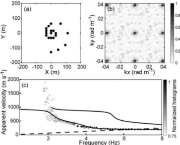
The frequency–wavenumber (f –k) based methods are often used for deriving the phase velocity dispersion curves from ambient vibration array measurements. In this study, we have used the conventional semblance-based f –k method CVFK (Kvaerna & Ringdahl 1986) implemented in the CAP software developed within the framework of the SESAME project (Ohrnberger 2004; Ohrnberger et al. 2004a,b). Operating with sliding time windows and narrow frequency bands, this method provides the wave prop-agation parameters (azimuth and slowness as a function of fre-quency) of the most coherent plane wave arrivals. In this study, we use a wavenumber grid layout sampled equidistantly in slowness and azimuth (azimuth and slowness sampling set to 5 degrees and 0.035 s km−1, respectively). The wave propagation characteristics were measured using 62 frequency bands between 1.8 and 8 Hz. The central frequency of each band was selected to be equally spaced in logarithm scale. A fraction of the central frequency fcdefined the frequency bandwidth (0.9 fc–1.1 fc). We selected the time-window length as seven times the central period corresponding to the analysed frequency band fcand used an overlap of 50 per cent in all frequency range between successive time windows. For the array analysis, we have considered a spiral shaped array composed of nineteen receivers. Only the vertical component of the noise syn-thetics is used for deriving the Rayleigh waves dispersion curve. The aperture of the array is about 200 m and the minimum distance between closer receivers is 16 m (Fig. 4a). The wavenumber valid-ity range of the array ranges between 0.0155 and 0.1963 rad m−1 (Fig. 4b).

The results from CVFK analysis are normalized histogram distri-butions in the frequency-slowness plane derived from the ensemble of wave propagation estimates obtained for each individual time– frequency cells. From the distributions however, we considered only the fourth quartile of both beam power and semblance highest es-timates and displayed the results in the frequency–velocity plane (grey and black circles displayed Fig. 4c). The theoretical disper-sion curves for fundamental and first higher Rayleigh waves modes are plotted for comparison. The maximum frequency that can be analysed by the array technique is defined by the spatial aliasing curve (C= 2π/kmax· f , with C the phase velocity, f the frequency

Figure 4. (a) Spatial location of the receivers (19 receivers in spiral

geom-etry) defined for the array analysis. (b) Normalized array transfer function for this spiral configuration. (c) Example of visualization of CVFK analysis results: velocities estimates are plotted versus frequency (circles), the grey and black scale for circles indicates the fourth quartile of the normalized histogram distributions derived from the ensemble of wave propagation es-timates obtained for each individual time–frequency cells; the black curves indicate the theoretical dispersion curves of the fundamental and the first higher mode of Rayleigh waves; the dashed line displays the spatial aliasing condition.

dminthe minimum distance between receivers), while the minimum

frequency is arbitrary defined by the resonance frequency of the site at 2 Hz. This lower limit is argued by multiple reasons. First, there is a filter effect by the sedimentary layer on noise vertical compo-nents (Scherbaum et al. 2003). The relative energy of noise vertical components is then smaller for frequencies below the resonance frequency than for frequencies above. Second, the noise simulation does not involve effects of very far sources such as coastal waves. Finally, the aperture of the array set up in this study is not designed such as to investigate low frequency.

4 W H I C H K I N D O F S O U R C E S F O R T H E A M B I E N T N O I S E ?

We will first present the results of our simulations, and then we will propose an interpretation of the relation between noise wavefield and H/V ratio.

4.1 Effects of source type

The first part of this work consists in investigating the influence of source time functions on H/V ratios. Do the H/V ratio peak charac-teristics (frequency and amplitude) depend on the characcharac-teristics of the source time functions?

Here, we consider only the R2 and B sources sets, respectively representative of local and far sources. We also consider that all sources are located at 2 m depth. For both sets of sources, noise synthetics have been computed at all receiver positions considering different sources type characteristics. In the first case, all source time functions are delta-like; in the second case we consider a mix between delta-like (50 per cent) and pseudo-monochromatic (50 per cent) source time functions (the proportions of source time functions are given according to the total number of sources in both sets); and

Figure 5. Mean H/V ratios (thick line) ± standard deviation (thin line)

computed using the M2 model of Table 1 for the (a) R2 sources set, (b) B sources set. (Top) 100 per cent delta-like time function; (middle) 50 per cent of delta-like and 50 per cent of pseudo-harmonic time functions (percentage in number of sources); (bottom) 100 per cent of pseudo-harmonic source time functions. All sources are located at 2 m depth.

in the third case all sources have pseudo-monochromatic source time functions. The mean H/V ratios obtained for local and far sources (R2 and B sources sets, respectively) computed with these different sources type are displayed in Fig. 5. The mean H/V ratio is calcu-lated using the individual H/V ratios obtained at the 290 receivers. In the three cases (delta-like sources, pseudo-monochromatic sources, or a mix of both sources types), H/V ratios computed from the R2 sources set show one clear dominant peak. Whatever the source time function, this peak is located at the fundamental resonance fre-quency of the layer (2 Hz). In case of mixed sources types however, H/V ratios exhibit a secondary low-amplitude peak located at a fre-quency close to 4 Hz. This is believed to be due to dominant Love waves, as discussed further in Section 5. The relative proportion of pseudo-harmonic and dirac source time function location may in-deed modify the relative contribution of Love-to-Rayleigh waves in the synthetic noise wavefield, and then modify the amplitude of the 4 Hz peak.

For far sources, the H/V ratios exhibit two clear peaks whatever the source time functions type considered: the first peak is located at the fundamental resonance frequency (2 Hz), and the second, sig-nificantly smaller than the previous one (two times in terms of peak amplitude), is located at the first higher harmonic of the S-wave resonance frequency. The existence of this second peak will be dis-cussed in Section 4.2. In both case (the R2 and B sources sets), the H/V ratio peak amplitudes (at the fundamental resonance and at the first harmonic) are weakly sensitive to the sources type.

In conclusion, we confirm conclusions of Lachet & Bard (1994), that is, the H/V ratio is weakly dependent on source time function type: its frequency is clearly independent, while the amplitude is weakly sensitive.

4.2 Effects of source distance

The second step of this study is to investigate the influence of the distance between sources and receivers on H/V ratios. According to the previous results on the effects of source type, noise synthetics

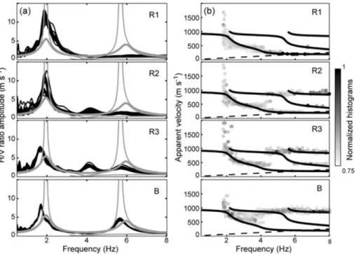
Figure 6. (a) H/V ratios computed using the M2 model of Table 1 at the array receivers (black curves) for four set of distance sources (R1, R2, R3, and B

sources). Thick grey curve displays the 1-D transfer function for vertically incident SH waves; thin grey curves display the ellipticity of the fundamental and the first higher modes of Rayleigh waves, respectively. (b) Apparent velocities (grey and black circles) estimated by the conventional f –k (CVFK) array method. The grey and black scale indicates the fourth quartile of the normalized histogram distributions derived from the ensemble of wave propagation estimates obtained for each individual time–frequency cells. Black curves represent the theoretical dispersion curves of the fundamental the first and the second harmonic of Rayleigh wave (plain lines), and the aliasing criteria (dashed lines). All sources are delta-like time functions located at 2 m depth.

have been computed considering only delta-like source time func-tions. All sources considered here are located at 2 m depth. Noise synthetics are computed separately for the four sources sets: R1, R2, R3, and B sources. We have performed array analysis on the nine-teen receivers (the spiral geometry) and we have computed the H/V ratios on the same nineteen receivers. H/V ratios and array analysis are displayed in Fig. 6.

In all cases, H/V ratios exhibit a peak around the fundamental resonance frequency at 2 Hz (Fig. 6a). For the R3 and B sources sets however, the H/V ratio peaks are shifted towards lower frequencies (1.7 Hz). Besides, for the R3 and B sources sets, H/V ratios also display another peak located at the first harmonic of the S-wave resonance frequency, that is, at 6 Hz (a small peak for the R3 sources set and a more significant one for the B sources set). It has also to be pointed out that H/V ratios for R2 and R3 sets also exhibit a third rather small peak located at 4 Hz, see Section 5 for further discussions.

For all sources sets, the array analysis (Fig. 6b) show a good fit, for frequency between 2 and 4 Hz, between the measured disper-sion curve and the theoretical disperdisper-sion curve of the fundamen-tal Rayleigh waves mode. Regarding the second H/V ratio peak at 6 Hz for the R3 and B sources sets, array analysis show that the noise wavefield is mainly composed of non-dispersive waves, with a phase velocity close to the S or Rayleigh waves velocity in the half-space.

All these observations may be summarized as follows: (1) for ambient noise due to local surface sources in one layer model, H/V ratios exhibit one peak located at the resonance frequency. At this frequency, fundamental mode of Rayleigh waves dominates the ver-tical ambient noise wavefield and (2) for noise due to far surface sources in a single layer over an half-space, H/V ratios exhibit two

peaks: the first peak is located at the fundamental resonance fre-quency (fundamental mode of Rayleigh waves dominate the verti-cal ambient noise wavefield at this frequency); the second one is located at the first harmonic (non-dispersive waves dominate the vertical noise wavefield at this frequency).

4.3 Effects of sources depth

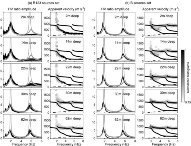
We now focus on the influence of source depth on the H/V ratio. We have selected the local and far sources sets (defined as the sum of the R1, R2 and R3 sources sets, and the B sources set, respectively), and all sources time functions are delta-like signals. We consider five sets of sources located respectively at 2, 14, 22, 30 and 62 m depth. The three first sets (at 2, 14 and 22 m depth) are located in-side the sediment layer, while the latest are located in the bedrock. Figs 7(a and b, left-hand side panel) show the H/V ratios computed at the nineteen receivers (left-hand side panel). In each case, H/V ratios exhibit a peak at the fundamental resonance frequency (2 Hz). How-ever, the origin of this peak strongly depends on sources location and depth as shown by the array analysis (Figs 7a and b, right-hand side panel). For local sources located inside the sedimentary layer, the computed dispersion curve fits with the dispersion curve of the theoretical fundamental mode of Rayleigh waves, outlining a noise vertical wavefield strongly dominated by Rayleigh waves. For far sources located within the sediment fill, the array analysis shows up the contribution of both Rayleigh and body waves in the vicinity of the resonance frequency; while at higher frequencies, non disper-sive waves dominate the vertical noise wavefield. For both far and local sources located within the bedrock, the array analysis indicates that the vertical noise wavefield is only composed by non-dispersive

Figure 7. H/V ratios computed using the M2 model of Table 1 at the array receivers (black curves), and apparent velocities estimated by the conventional f –k

(CVFK) array method, (a) for local sources (sum of the R1, R2 and R3 sources set) and (b) far sources (B sources set), located inside the layer (2, 14 and 22 m depth), and located below the sedimentary layer (30 and 62 m depth). See Fig. 6 for legend.

waves whatever the frequency (their velocity is equal to the S-wave velocity in the bedrock).

An H/V peak at 6 Hz is systematically observed when sources are far whatever their depth, or when sources are located within the bedrock. In each case, body waves, having a S-wave velocity equals to the bedrock S-wave velocity, dominate the vertical wavefield. Moreover, at the resonance frequency (2 Hz) and at the first harmonic of the resonance frequency (6 Hz), in case of sources located within the bedrock, the shape of the H/V curves fit well the shape of the 1-D transfer function curve (in terms of frequency peak and amplitude peak). In this case, the H/V ratios peaks are related to the S-wave resonance.

These last observations can be summarized and interpreted as follows:

(1) for ambient noise due to local sources within the sedimen-tary layer, H/V ratios exhibit only one strong peak located at the fundamental resonance frequency. The corresponding vertical noise wavefield is dominated by the fundamental mode of Rayleigh waves, and H/V peak is most probably due to the ellipticity of the funda-mental mode of Rayleigh waves;

(2) for ambient noise due to far sources within the layer, H/V ra-tios exhibit two peaks, one is located at the resonance frequency and is produce by a mixture of fundamental Rayleigh waves and to non-dispersive waves. The other one that occurs at the first harmonic frequency of the resonance is due to non-dispersive waves, this could be produced by S head waves along the sediment-to-bedrock interface;

(3) for ambient noise due to sources located within the bedrock, H/V ratios exhibit two peaks at the fundamental and the first har-monic resonance frequencies; the vertical noise wavefield is strongly dominated by S waves. H/V ratios peaks are related to multiple

S-waves resonance.

5 D I S C U S S I O N

In order to validate the interpretation expressed in the above section, two ‘extreme’ (and unrealistic) models (M3 and M4) have been built. These models are based on the M2 model (same thickness, same body wave velocities, same density), the only difference between models M3 and M4 is the quality factor value (Table 2). In the M3 model, we impose very low attenuation in the upper layer (quality factors equal to 1000), and a strong attenuation in the half-space (quality factors equal to 10). On the contrary, in the M4 model, there is a strong attenuation in the upper layer (quality factors equal to 10) and no attenuation in the half-space (quality factors equal to 1000). Only far sources modelled with delta-like time functions and located at 2 m depth, are considered here.

According to these extreme values for the attenuation, the fol-lowing wavefield characteristics may be expected: (1) for the M3 model, there should be no attenuation of surface waves within the layer, and they should propagate over larger distances. On the con-trary, the head waves should be strongly attenuated and thus should not contribute so much to the noise wavefield for intermediate to large distances; (2) for the M4 model, only a very small amount of

Table 2. Physical parameters for the ‘extreme’ models, M3 and M4 (models

based on the M2 model, with different attenuation properties).

Thickness Vp Vs Rho Qp Qs (m) (m s−1) (m s−1) (Kg m−3) M3 model Sediments 25 1350 200 1.9 1000 1000 Bedrock infinite 2000 1000 2.5 10 10 M4 model Sediments 25 1350 200 1.9 10 10 Bedrock infinite 2000 1000 2.5 1000 1000

surface waves should propagate within the sediment layer because of the large attenuation. The wavefield should thus be dominated by head waves that propagate over large distances along the sediment-to-bedrock interface.

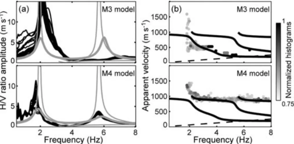
Fig. 8 shows the H/V and array analysis results for the M3 and the M4 model. As expected, for the M3 model, H/V ratio exhibits only one peak located at the fundamental resonance frequency due to the ellipticity of fundamental Rayleigh waves. No peak at 6 Hz as it was previously observed for the M2 model with the same source–receiver configuration is observed. This observation strongly supports the fact that the H/V ratio peak at 6 Hz on the M2 model is due to resonating head waves. For the M4 model, H/V ratios exhibit two peaks at the fundamental and the first higher mode of the resonance frequency. According to the array analysis, non-dispersive waves dominate the wavefield at these frequencies. Since there is a strong attenuation in the upper layer, surface waves cannot easily propagate in the layer, thus H/V peaks are due to head S waves that propagate at the sediment-to-bedrock interface.

These results support the interpretation of the origin of H/V peaks expressed in the above section, and can be summarized as follows: (1) if sources are inside the sedimentary layer and far away, H/V ratio shows two peaks. One is due to fundamental Rayleigh waves and resonating head S waves; the second one is due to head waves; (2) if sources are inside the sedimentary layer, H/V ratio shows one single peak due to horizontal ellipticity of fundamental Rayleigh waves.

Going back to the H/V actually observed, one may notice that H/V curves most generally exhibit one peak at the fundamental

Figure 8. (a) H/V ratios computed at the arrays receivers (black curves) for far sources (B sources set located at 2 m depth) for the following ‘extreme case’: no

attenuation in the upper layer and strong attenuation in the half-space (M3 model, top); strong attenuation in the upper layer and no attenuation in the half-space (M4 model, bottom) (see Table 2). (b) Apparent velocities estimated by the conventional f –k (CVFK) array method. See Fig. 6 for legend.

resonance frequency (Duval 1994; Ansary et al. 1995; Bard 1998; Volant et al. 1998; Cara et al. 2003). According to our simulation this case occurs only when sources are rather close to the receivers and located within the sediment. In cases of far sources or sources located within the bedrock, two H/V peaks show up at the funda-mental and the first higher resonance modes. When actual noise measurements are performed, far and close sources obviously con-tribute to the noise wavefield. Noise synthetics generated by all the sources sets (i.e. the sum of the R1, R2, R3 and B sources) have then been summed up. The H/V and array analysis performed on these noise synthetics outline the ‘control’ of the local sources on the re-sulting H/V curves and array analysis estimates (Fig. 9). The H/V curve indeed exhibits only one peak at the fundamental resonance frequency and the vertical noise wavefield is strongly dominated by Rayleigh waves. These results thus strongly suggest the importance of local sources in controlling the wavefield main properties. This numerical experiment, close to field measurements (noise sources located at various distances), agrees with field experiments showing that observed H/V ratios exhibit, usually, only one peak. Note that this statement is true in a majority of cases, but multiple peaks on H/V curves have been sometimes reported (Gu´eguen et al. 1998; Bodin et al. 2001; Lebrun et al. 2001; Woolery & Street 2002; As-ten 2004; Oliveto et al. 2004). For example, Bodin et al. (2001) have observed and documented two higher peaks in a large set of H/V data in the Mississippi basin. Discussion by Asten (2004) suggested one peak was due to the horizontal polarization of the first higher mode of Rayleigh waves, while another was a fundamental mode as-sociated with a very soft surficial layer. These observations illustrate that the identification of the H/V higher peaks is not straightforward in the field.

Our numerical results are also supported by Parolai & Galiana-Merino (2006). Although these authors considered the variability of the H/V ratio as a function of distance for only one point source, the results are comparable (e.g. the presence of a secondary peak at certain distance ranges and for certain source directions), at least for a first approximation.

As it has been previously mentioned, H/V curves computed for the R2 and R3 source sets exhibit a low amplitude peak at 4 Hz. In order to determine the origin of this peak, we computed noise synthetics at receivers linearly equispaced along the X -axis from the B sources area, as displayed in Fig. 10(a). Sources are located at 2 m depth and

Figure 9. (a) H/V ratios computed using the M2 model of Table 1 at the array receivers (black curves) for all sources (the sum of the R1, R2, R3, and B sources

sets). Sources were located at 2 m depth. (b) Apparent velocities estimated by the conventional f –k (CVFK) array method. See Fig. 6 for legend.

Figure 10. (a) Sources (stars) and receivers (dots) locations. (b) Love to Rayleigh waves energy density ratio contribution computed from equation (1) for

the M2 model (see Table 1). The amplitude ratio is plotted in logarithm scale; the minimum value is represented in white colour, and the maximum value in black. (c) Relative energy density contribution for Rayleigh (dashed line) and Love (plain line) waves computed for a uniform source distribution at 4 Hz. H/V peak frequencies calculated for the ambient noise synthetics computed at each receiver position for random sources, note that only peak frequencies exhibiting amplitude higher than 2 are plotted: (d) H/V ratio calculated with both horizontal components, (e) H/V ratio calculated with the Fourier spectra amplitude along the X direction (X/V), (f) H/V ratio calculated with the Fourier spectra amplitude along the Y direction (Y/V).

the M2 model (Table 1) is considered. H/V peak frequencies having amplitudes higher than two were picked and displayed in Fig. 10(d). The 4 Hz H/V peak is observed when the source–receiver distance ranges from 300 to 800 m. Following Ohrnberger (2005) the Love to Rayleigh waves energy density ratio (RL/R) can be expressed as follows:

RL/R= e

(−2·π· f ·x)/(CL·Q)

e(−2·π· f ·x)/(CR·Q), (1)

where f is the frequency, x the source–receiver distance, Q the shear-wave quality factor and CR, CLthe group velocities of Rayleigh and

Love waves, respectively. Fig. 10(b) shows the normalized Love to Rayleigh waves energy density ratio derived from the M2 model and computed following (1). A predominant contribution of Love waves compared to Rayleigh waves is observed at 4 Hz, and from source–receiver distances larger than 100 m. In case of modelling only surface waves, a 4 Hz H/V peak should thus be observed for source-to-receiver distances larger than 100 m. However, in our simulation, the 4 Hz peak is not appearing anymore for source-to-receivers distance larger than 900 m. This may be explained by the contribution of head waves that counter-balance the contribution of Rayleigh and Love waves that carry very low and insignificant

energy for large source-to-receivers distance (Fig. 10c). Moreover, when spectra of X/V and Y/V are calculated separately (with X, Y, and Z the Fourier spectra amplitude along the X , Y and Z directions, respectively), the 4 Hz H/V peak is observed only in the second case (i.e. Y/V spectral ratio) and for source–receiver distances range between 250 and 1000 m (Fig. 10e and f). Besides, when H/V ratios are calculated from noise synthetics computed with only vertical sources, the H/V curves do not exhibit peak at 4 Hz (not shown here). Then, at 4 Hz and for source–receiver distances range between 300 and 800 m, the strong contribution of Love waves compared to Rayleigh waves may explain the origin of the 4 Hz peak observed on H/V ratio curves. Note that, in (1), the quality factor is assumed to be equal to the S wave one. This approximation is true because of the large P- to S-wave velocity ratio defined in the particular case of the M2 model (see Table 1). Therefore one has to be cautious when using (1) in case of other soil structures. The generalization of (1) is out of the scope of the present paper.

6 C O N C L U S I O N

We have simulated ambient seismic noise for a simple 1-D structure (one layer over a half-space) in order to thoroughly test the H/V technique for well-controlled conditions and investigate the compo-sition of noise wavefield around the H/V peak frequency. We have performed a parametric study of the effects of the source distribution (time function, spatial location (in 3-D plane)) on H/V ratio shapes. The first conclusion outlined by this study is the independence of the H/V ratio regarding the source time functions. We show that the H/V frequency peak is clearly independent on source time functions, while the peak amplitude is only weakly sensitive.

Moreover, we can synthesize the effects of spatial location of sources on H/V ratio shape as follows:

(1) if ambient noise sources are in the bedrock, H/V ratio peaks are due to S-wave resonance of the head waves;

(2) if ambient noise sources are inside the sedimentary layer and far away, H/V ratio shows up two peaks. One is due to fundamental mode of Rayleigh waves and resonating head S waves; the second one is due to head waves;

(3) if ambient noise sources are close and inside the sedimen-tary layer, H/V ratio shows one peak due to horizontal ellipticity of fundamental mode of Rayleigh waves.

Note that as the present results have been demonstrated only for the seismic noise vertical component we cannot state about the con-tribution of Love waves to the H/V ratio.

The main result outlined by this study is the control of the local sources on the H/V shape which is in agreement with the actual H/V ratios that most of the times exhibit only one peak. Even if we show that in some cases (far and/or deep sources), H/V ratio can exhibit more than one peak, the contribution of these sources to the noise wavefield is rather small. Subsequently, the vertical noise wavefield, at the fundamental resonance frequency, is mainly composed of Rayleigh waves (in one sedimentary layer over bedrock). Thus the amplitude of the H/V ratios peak cannot be used to reach a good estimate of the site amplification factor. This interpretation is in agreement with previous studies which show that surface waves dominated the noise wavefield (Horike 1985; Arai & Tokimatsu 1998). Note that results presented here are done for a given soil model. To enhance these conclusions it is now necessary to perform similar parametric study on other type of structures such as multiple sedimentary layers with various impedance contrasts (see Asten

& Dhu 2004; Dolenc & Dreger 2005) and/or quality factors, and 3-D structures as sedimentary valley or rough interface between sediment and bedrock (see Cornou 2005; Roten et al. 2006).

To go ahead in the investigation of the nature of noise wavefield it would be interesting to use the 3-components array techniques such as the three-component SPAC method (Aki 1957). This method should allow us to determine the relative proportion of Rayleigh and Love waves in noise wavefield, and therefore it should be a helpful tool to better understand the influence of Love waves on H/V curves, especially at the Loves waves Airy phase frequency. One can refer to the works done by Arai & Tokimatsu (1998), Yamamoto (2000), Okada (2003), K¨ohler et al. (2006) or Bonnefoy-Claudet

et al. (2006) showing that the relative proportion of Love waves in

the seismic noise wavefield varies from site to site.

This study also shows that, in case of far ambient noise sources, H/V ratios peaks can be exhibited at the harmonics resonance fre-quencies (not only at the fundamental resonance frequency). It then may be possible to perform ambient field noise measurement in or-der to fill the conditions which allow the harmonic resonance peaks frequencies to be characterized. Further numerical and experimen-tal works are now in process in order to give a clear assessment of the ability of the H/V method in such cases.

A C K N O W L E D G M E N T S

We thank Matthias Ohrnberger and Marc Wathelet for providing the array software. We thank the participants of the SESAME project for helpful discussions, comments and suggestions. This work was partly supported by the EU research program Energy, Environment and Sustainable Development (EC-contract No: EVG1-CT-2000-00026), and also partly funded by European Union through EU-ROSEISRISK project, contract EVG1-CT-2001-00040. Most of the computations were performed at the Service Commun de Calcul Intensif de l’Observatoire de Grenoble (SCCI) France and at the Swiss Center for Scientific Computing (SCSC).

R E F E R E N C E S

Aki, K., 1957. Space and time spectra of stationary stochastic waves, with special reference to microtremors, Bull. Earthquake. Res. Inst. Tokyo, 35, 415–457.

Al Yuncha, Z. & Luzon, F., 2000. On the horizontal-to-vertical spectral ratio in sedimentary basins, Bull. seism. Soc. Am., 90, 1101–1106.

Ansary, M.A., Yamazaki, F., Fuse, M. & Katayama, T., 1995. Use of mi-crotremors for the estimation of ground vibration characteristics, Third

international conferences on recent advances in geotechnical earthquake engineering and soil dynamics, St. Louis, Missouri, 2.

Arai, H. & Tokimatsu, K., 1998. Evaluation of local site effects based on microtremor H/V spectra, Proceeding of the Second International

Sym-posium on the Effects of Surface Geology on Seismic Motion, Yokohama,

Japan, 2, 673–680.

Asten, M.W., 2004. Comment on ‘Microtremor observations of deep sed-iment resonance in metropolitan Memphis, Tennessee’ by Paul Bodin, Kevin Smith, Steve Horton and Howard Hwang, Engineering Geology,

72, 343–349.

Asten, M.W. & Dhu, T., 2004. Site response in the Botany area, Sydney, using microtremor array methods and equivalent linear site response modelling,

Proceedings of a conference of the Australian Earthquake Engineering Society, Mt Gambier South Australia.

Bard, P.-Y., 1998. Microtremor measurements: a tool for site effect estima-tion? Proceeding of the Second International Symposium on the Effects

Bodin, P., Smith, K., Horton, S. & Hwang, H., 2001. Microtremor observa-tions of deep sediment resonance in metropolitan Memphis, Tennessee,

Engineering Geology, 2, 159–168.

Bonnefoy-Claudet, S., Cotton, F. & Bard, P.-Y., 2006. The nature of seismic noise wavefield and its implications for site effects studies. A literature review, Earth-Sci. Rev., in press (doi: 10.1016/j.earscirev. 2006.07.004).

Bour, M., Fouissac, D., Dominique, P. & Martin, C., 1998. On the use of microtremor recordings in seismic microzonation, Soil Dyn. and Earthq.

Eng., 17, 465–474.

Cara, F., Di Giulio, G. & Rovelli, A., 2003. A study on seismic noise varia-tions at Colfiorito, central Italy: implicavaria-tions for the use of H/V spectral ratios, Geophys. Res. Lett., 30, 1972.

Cornou, C., 2005. Simulation for real sites, SESAME Report D17.10 (http://sesame-fp5.obs.ujf-grenoble.fr).

Di Giulio, G., Rovelli, A., Cara, F., Azzara, R.M., Marra, F., Basili, R. & Caserta, A., 2003. Long-duration asynchronous ground motions in the Colfiorito plain, central Italy, observed on a two-dimensional dense array,

J. geophys. Res., 108, 2486–2500.

Dolenc, D. & Dreger, D., 2005. Microseisms observations in the Santa Clara Valley, California, Bull. seism. Soc. Am., 95, 1137–1149.

Duval, A.-M., 1994. D´etermination de la r´eponse d’un site aux s´eismes `a l’aide du bruit de fond: ´evaluation exp´erimentale, PhD thesis, Universit´e Pierre-et-Marie Curie, Paris, France. (In French with English asbtract) F¨ah, D., 1997. Microzonation of the city of Basel, J. Seism., 1, 87–102. F¨ah, D., Kind, F. & Giardini, D., 2001. A theoretical investigation of average

H/V ratios, Geophys. J. Int., 145, 535–549.

Field, E. & Jacob, K., 1993. The theoretical response of sedimentary layers to ambient seismic noise, Geophys. Res. Lett., 20, 2925–2928. Fukushima, Y., Kinoshita, S. & Sato, H., 1992. Measurement of Q for

S-wave in mudstone at Chikura, Japan: comparison of incident and reflected phases in boreholes seismograms, Bull. seism. Soc. Am., 82, 148–163. Gitterman, Y., Zaslavsky, Y., Shapira, A. & Shtivelman, V., 1996. Empirical

site response evaluations: case studies in Israel, Soil Dyn. and Earthq.

Eng., 15, 447–463.

Gu´eguen, P., Chatelain, J.-L., Guillier, B., Yepes, H. & Egred, J., 1998. Site effect and damage distribution in Pujili (Ecuador) after the 28 march 1996 earthquake, Soil Dyn. and Earthq. Eng., 17, 329–334.

Hauksson, K., Teng, T. & Henyey, T.L., 1987. Results from a 1500 m deep, three-level downhole seismometer array: site response, low Q value, and

fmax, Bull. seism. Soc. Am., 77, 1883–1904.

Hisada, Y., 1994. An efficient method for computing Green’s functions for a layered half-space with sources and receivers at close depths, Bull. seism.

Soc. Am., 84, 1456–1472.

Hisada, Y., 1995. An efficient method for computing Green’s functions for a layered half-space with sources and receivers at close depths (Part 2),

Bull. seism. Soc. Am., 85, 1080–1093.

Horike, M., 1985. Inversion of phase velocity of long-period microtremors to the S-wave-velocity structure down to the basement in urbanized areas,

J. Phys. Earth, 33, 59–96.

Jongmans, D. et al., 1998. EUROSEISTEST: determination of the geological structure of the Volvi basin and validation of the basin response, Bull.

seism. Soc. Am., 88, 473–487.

K¨ohler, A., Ohrnberger, M. & Scherbaum, F., 2006. The relative fraction of Rayleigh and Love waves in ambient vibration wavefields at differ-ent European sites. Proceedings of the third International Symposium on the Effects of Surface Geology on Seismic Motion, Grenoble, France,

Geophys. J. Int., submitted.

Konno, K. & Ohmachi, T., 1998. Ground-motion characteristics estimated from spectral ratio between horizontal and vertical components of mi-crotremor, Bull. seism. Soc. Am., 88, 228–241.

Kudo, K., 1995. Practical estimates of site response. State-of-art report,

Proceedings of the fifth International Conference on Seismic Zonation,

Nice, France.

Kvaerna, T. & Ringdahl, F., 1986. Stability of various f-k estimation tech-niques, Semiannual Technical Summary, NORSAR Scientific Report, 29– 40.

Lachet, C. & Bard, P.-Y., 1994. Numerical and theoretical investigations on

the possibilities and limitations of Nakamura’s technique, J. Phys. Earth,

42, 377–397.

Lebrun, B., Hatzfeld, D. & Bard, P.-Y., 2001. Site effect study in urban area: experimental results in Grenoble (France), Pure appl. Geophys.,

158, 2543–2557.

Lermo, J. & Chavez-Garcia, F.J., 1993. Site effects evaluation using spectral ratios with only one station, Bull. seism. Soc. Am., 83, 1574–1594. Lermo, J. & Chavez-Garcia, F.J., 1994. Site effect evaluation at Mexico

city: dominant period and relative amplification from strong motion and microtremor records, Soil Dyn. and Earthq. Eng., 13, 413–423. Malischewsky, P. & Scherbaum, F., 2004. Love’s formula and H/V-ratio

(ellipticity) of Rayleigh waves, Wave Motion, 40, 57–67.

Maresca, R., Castellano, M., De Matteis, R., Saccorotti, G. & Vaccariello, P., 2003. Local site effects in the town of Benevento (Italy) from noise measurements, Pure appl. Geophys., 160, 1745–1764.

McNamara, D. & Buland, R., 2004. Ambient noise levels in the continental United States, Bull. seism. Soc. Am., 94(4), 1517–1527.

Moczo, P. & Kristek, J., 2002. FD code to generate noise synthetics, SESAME

report D02.09 (http://sesame-fp5.obs.ujf-grenoble.fr).

Mucciarelli, M., 1998. Reliability and applicability of Nakamura’s technique using microtremors: an experimental approach, J. Earthq. Eng., 2, 625– 638.

Nakamura, Y., 1989. A method for dynamic characteristics estimation of subsurface using microtremor on the ground surface, Quaterly Report

Railway Tech. Res. Inst., 30, 25–30.

Nakamura, Y., 1996. Real-time information systems for hazards mitigation,

Proceedings of the 11th World Conference on Earthquake Engineering,

Acapulco, Mexico.

Nakamura, Y., 2000. Clear identification of fundamental idea of Nakamura’s technique and its applications, Proceedings of the 12th World Conference

on Earthquake Engineering, Auckland, New Zealand.

Nogoshi, M. & Igarashi, T., 1971. On the amplitude characteristics of mi-crotremor (part 2), J. Seismol. Soc. Japan, 24, 26–40. (In Japanese with English abstract)

Ohrnberger, M., 2004. User manual for software package CAP—a continu-ous array processing toolkit for ambient vibration array analysis, SESAME

report D18.06 (http://sesame-fp5.obs.ujf-grenoble.fr).

Ohrnberger, M., 2005. Report on FK/SPAC capabilities and limitations,

SESAME report D19.06 (http://sesame-fp5.obs.ujf-grenoble.fr).

Ohrnberger, M., Schissele, E., Cornou, C., Bonnefoy-Claudet, S., Wathelet, M., Savvaidis, A., Scherbaum, F. & Jongmans, D., 2004a. Frequency wavenumber and spatial autocorrelation methods for dispersion curve determination from ambient vibration recordings, Proceedings of the

13th World Conference on Earthquake Engineering, Vancouver, Canada,

Paper 946.

Ohrnberger, M., Schissele, E., Cornou, C., Wathelet, M., Savvaidis, A., Scherbaum, F., Jongmans, D. & Kind, F., 2004b. Microtremor array mea-surements for site effect investigations: comparison of analysis methods for field data crosschecked by simulated wavefields, Proceedings of the

13th World Conference on Earthquake Engineering, Vancouver, Canada,

Paper 940.

Okada, H., 2003. The Microtremor Survey Method, Geophysical Monograph Series, 12, Society of exploration geophysicists, Tulsa.

Oliveto, A., Mucciarelli, M. & Caputo, R., 2004. HVSR prospecting in multi-layered environments: an example from the Tyrnavos Basin (Greece), J.

Seism., 8, 395–406.

Parolai, S. & Galiana-Merino, J., 2006. Effect of transient seismic noise on estimates of H/V spectral ratios, Bull. seism. Soc. Am., 96, 228–236. Rodriguez, H.S. & Midorikawa, S., 2003. Comparison of spectral ratio

tech-niques for estimation of site effects using microtremor data and earthquake motions recorded at the surface and in boreholes, Earthq. Eng. Struct.

Dyn., 32, 1691–1714.

Roten, D., F¨ah, D., Cornou, C. & Giardini, D., 2006. Two-dimensional res-onances in Alpine valleys identified from ambient vibration wavefields,

Geophys. J. Int. 165, 889–905.

Scherbaum, F., Hinzen, K.-G. & Ohrnberger, M., 2003. Determination of shallow shear wave velocity profiles in the Cologne/Germany area using ambient vibrations, Geophys. J. Int., 152, 597–612.

Seekins, L.C., Wennerberg, L., Marghereti, L. & Liu, H.-P., 1996. Site am-plification at five locations in San Fransico, California: a comparison of S waves, codas, and microtremors, Bull. seism. Soc. Am., 86, 627–635. Tokeshi, J.C. & Sugimura, Y., 1998. On the estimation of the natural period

of the ground using simulated microtremors, Proceeding of the Second

International Symposium on the Effects of Surface Geology on Seismic Motion, Yokohama, Japan, 2, 651–664.

Tokimatsu, K., 1997. Geotechnical site characterization using surface waves, Proceedings of the First International Conference on Earthquake

Geotechnical Engineering, 3, 1333–1368.

Volant, P., Cotton, F. & Gariel, J.-C., 1998. Estimation of site response using the H/V method. Applicability and limits of this technique on Garner Val-ley downhole array dataset (California), Proceedings of the 11th European

Conference on Earthquake Engineering, Paris.

Wakamatsu, K. & Yasui, Y., 1996. Possibility of estimation for amplification characteristics of soil deposits based on ratio of horizontal to vertical spectra of microtremors, Proceedings of the 11th World Conference on

Earthquake Engineering, Acapulco, Mexico.

Wang, Z., Street, R. & Woolery, E., 1994. Qs estimation for unconsolidated sediments using first-arrival SH critical refractions, J. geophys. Res., 99, 13 543–13 551.

Woolery, E. & Street, R., 2002. 3D near-surface soil response from H/V ambient-noise ratios, Soil Dyn. and Earthq. Eng., 22, 865– 876.

Yamamoto, H., 2000. Estimation of shallow S-wave velocity structures from phase velocities of love and Rayleigh waves in microtremors, Proceedings

of the 12th World Conference on Earthquake Engineering, Auckland, New