HAL Id: halshs-01322844
https://halshs.archives-ouvertes.fr/halshs-01322844
Submitted on 27 May 2016
HAL is a multi-disciplinary open access
archive for the deposit and dissemination of
sci-entific research documents, whether they are
pub-lished or not. The documents may come from
teaching and research institutions in France or
abroad, or from public or private research centers.
L’archive ouverte pluridisciplinaire HAL, est
destinée au dépôt et à la diffusion de documents
scientifiques de niveau recherche, publiés ou non,
émanant des établissements d’enseignement et de
recherche français ou étrangers, des laboratoires
publics ou privés.
Distributed under a Creative Commons Attribution - NonCommercial - NoDerivatives| 4.0
International License
User-Based Solutions for Increasing Level of Service in
Bike-Sharing Transportation Systems
Juste Raimbault
To cite this version:
Juste Raimbault. User-Based Solutions for Increasing Level of Service in Bike-Sharing Transportation
Systems. Complex Systems Design & Management Proceedings of the Fifth International Conference
on Complex Systems Design & Management CSD&M 2014, 2015, 978-3-319-11617-4.
�10.1007/978-3-319-11617-4_3�. �halshs-01322844�
service in bike-sharing transportation systems
Juste Raimbault
Graduate School, Ecole Polytechnique, Palaiseau, France
and LVMT, Ecole Nationale des Ponts et Chauss´ees,
Champs-sur-Marne, France juste.raimbault@polytechnique.edu
Abstract. Bike-sharing transportation systems have been well studied from a top-down viewpoint, either for an optimal conception of the sys-tem, or for a better statistical understanding of their working mecha-nisms in the aim of the optimization of the management strategy. Yet bottom-up approaches that could include behavior of users have not been well studied so far. We propose an agent-based model for the short time evolution of a bike-sharing system, with a focus on two strategical pa-rameters that are the role of the quantity of information users have on the all system and the propensity of user to walk after having dropped their bike. We implement the model in a general way so it is applicable to every system as soon as data are available in a certain format. The model of simulation is parametrized and calibrated on processed real time-series of bike movements for the system of Paris. After showing the robustness of the simulations by validating internally and externally the model, we are able to test different user-based strategies for an increase of the level of service. In particular, we show that an increase of user information can have significant impact on the homogeneity of repartition of bikes in docking stations, and, what is important for a future implementation of the strategy, that an action on only 30% of regular users is enough to obtain most of the possible amelioration.
Keywords: bike-sharing transportation system, agent-based modeling, bottom-up complex system management
1
Introduction
Bike-sharing transportation systems have been presented as an ecological and user-friendly transportation mode, which appears to be well complementary to classic public transportation systems ([1]). The quick propagation of many im-plementations of such systems across the world confirms the interesting poten-tialities that bike-sharing can offer [2]. O’Brien & al. propose in [3] a review on the current state of bike-sharing across the world. Inspired by the relatively good success of such systems in Europe, possible key factors for their quality have been questioned and transposed to different potential countries such as China ([4, 5]) or the United States ([6]).
The understanding of system mechanisms is essential for its optimal exploita-tion. That can be done through statistical analysis with predictive statistical models ([7–10]) or data-mining techniques ([3, 11]), and can give broader results such as structure of urban mobility patterns. Concerning the implementation, a crucial point in the design of the system is an optimal location of stations. That problem have been extensively studied from an Operational Research point of view ([12, 13] for example). The next step is a good exploitation of the system. By nature, strong asymmetries appear in the distribution of bikes: docking sta-tions in residential areas are emptied during the day contrary to working areas. That causes in most cases a strong decrease in the level of service (no parking places or no available bikes for example). To counter such phenomena, operators have redistribution strategies that have also been well studied and for which optimal plans have been proposed ([14–16]).
However, all these studies always approach the problem from a top-down point of view, in the sense of a centralized and global approach of the issues, whereas bottom-up strategies (i. e. local actions that would allow the emergence of desired patterns) have been to our knowledge not much considered in the literature. User-based methods have been considered in [17, 18] in the case of a car-sharing system, but the problem stays quite far from a behavioral model of the agents using the system, since it explores the possibility of implication of users in the redistribution process, or of shared travels what is not relevant in the case of bikes. Indeed the question of a precise determination of the influ-ence of users behaviors and parameters on the level of service of a bike-sharing systems remains open. We propose an agent-based model of simulation in order to represent and simulate the system from a bottom-up approach, considering bikers and parking as stations as agents and representing their interactions and evolutions in time. That allows to explore user-targeted strategies for an increase of the level of service, as the incitation to use online information media or to be more flexible on the destination point. Note that our work aims to explore effects of user-based policies, but does not pretend to give recommendations to system managers, since our approach stays technical and eludes crucial political and human aspects that one should take into account in a broader system design or management context.
The rest of the paper is organized as follows. The model and indicator used to quantify its behavior are described in Section 2. Next, Section 3 presents the implementation and results, including internal and external validations of the model by sensitivity analysis and simplified calibration on real data, and also exploration of possible bottom-up strategies for system management. We conclude by a discussion on the applicability of results and on possible develop-ments.
2
Presentation of the model
Introduction The granularity of the model is the scale of the individual biker and of the stations where bikes are parked. A more integrated view such as
flows would not be useful to our purpose since we want to study the impact of the behavior of individuals on the overall performance of the system. The global working scheme consists in agents embedded in the street infrastructure, interacting with particular elements, what is inspired from the core structure of the Miro model ([19]). Spatial scale is roughly the scale of the district; we don’t consider the whole system for calculation power purposes (around 1300 stations on all the system of Paris, whereas an interesting district have around 100 stations), what should not be a problem as soon as in- and outflows allow to reconstruct travels entering and getting out of the area. Tests on larger spatial zones showed that generated travel were quite the same, justifying this choice of scale. Focusing on some particular districts is important since issues with level of service occur only in narrow areas. Time scale of a run is logically one full day because of the cyclic nature of the process ([20]).
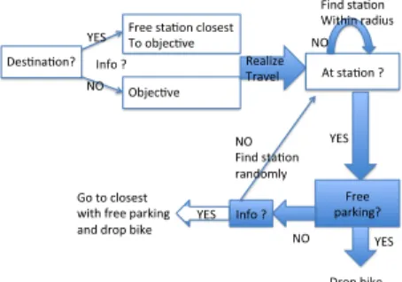
Des$na$on? Info ? YES NO
Free sta$on closest To objec$ve Objec$ve
Realize
Travel At sta$on ? NO Find sta$on Within radius YES Free parking? YES Drop bike NO Info ? NO Find sta$on randomly YES Go to closest with free parking and drop bike
Fig. 1: Flowchart of the decision process of bikers, from the start of their travel to the drop of the bike.
Formalisation The street network of the area is an euclidian network (V ⊂ R2, E ⊂ V × V ) in a closed bounded part of R2. The time is
discretized on a day, so all temporal evolu-tion are defined on T = [0, 24] ∩ τ N with τ time step (in hours). Docking stations S are particular vertices of the network for which constant capacities c(s ∈ S) are defined, and that can contain a variable number of bikes pb(s) ∈ {0, . . . , c}T. We suppose that
tem-poral fields O(x, y, t) and D(x, y, t) are de-fined, corresponding respectively to probabili-ties that a given point at a given time becomes the expected departure (resp. the expected ar-rival) of a new bike trip, knowing that a trip
starting (resp. arriving) at that time exists. Boundaries conditions are repre-sented as a set of random variables (NI(i, t)). For each possible entry point i ∈ I
(I ⊂ V is a given set of boundaries points) and each time, NI(i, t) gives the
number of bikes trips entering the zone at point i and time t. For departures, a random time-serie ND(t) represents the number of departures in the zone at
time t. Note that these random variables and probabilities fields are sufficient to built the complete process of travel initiation at each time step. Parametrization of the model will consist in proposing a consistent way to construct them from real data.
Docking stations are fixed agents, only their functions pb will vary through
time. The other core agents are the bikers, for which the set B(t) is variable. A biker b ∈ B(t) is represented by its mean speed ¯v(b), a distance r(b) correspond-ing to its “propensity to walk” and a boolean i(b) expresscorrespond-ing the capacity of having access to information on the whole system at any time (through a mobile device and the dedicated application for example). The initial set of bikers B(0) is taken empty, as t = 0 corresponds to 3a.m. when there is approximately no travels on standard days.
We define then the workflow of the model for one time step. The following scheme is sequentially executed for each t ∈ T , representing the evolution of the system on a day.
For each time step the evolution of the system follows this process :
– Starting new travels. For a travel within the area, if biker has information, he will adapt his destination to the closest station of its destination with free parking places, if not his destination is not changed.
• For each entry point, draw number of new traveler, associate to each a destination according to D and characteristics (information drawn uni-formly from proportion of information, speed according to fixed mean speed, radius also).
• Draw new departures within the area according to O, associate either destination within (in proportion to a fixed parameter pit, proportion of
internal travels) the area, or a boundary point (travel out of the area). If the departure is empty, biker walks to an other station (with bikes if has information, a random one if not) and will start his travel after a time determined by mean walking speed and distance of the station. • Make bikers waiting for start for which it is time begin their journey
(correspond to walkers for which a departure station was empty at a given time step before)
– Make bikers advance of the distance corresponding to their speed. Travel path is taken as the shortest path between origin and destination, as effective paths are expected to have small deviation from the shortest one in urban bike travels [8].
– Finish travels or redirect bikers
• if the biker was doing an out travel and is on a boundary point, travel is finished (gets out of the area)
• if has no information, has reached destination and is not on a station, go to a random station within r(b)
• if is on a station with free places, drop the bike
• if is on a station with no places, choose as new destination either the clos-est station with free places if he has information, or a random one within r(b) (excluding already visited ones, implying the memory of agents).
Fig. 1 shows the decision process for starting and arriving bikers. Note that walking radius r(b) and information i(b) have implicitly great influence on the output of the model, since dropping station is totally determined (through a random process) by these two parameters when the destination is given.
Evaluation criteria In order to quantify the performance of the system, to com-pare different realizations for different points in the parameter space or to evalu-ate the fitness of a realization towards real data, we need to define some functions of evaluation, proxies of what are considered as “qualities” of the system.
Temporal evaluation functions These are criteria evaluated at each time step and for which the output on the all shape of the time-series will be compared.
– Mean load factor ¯l(t) =|S|1 P
s∈S pb(s)
c(s)
– Heterogeneity of bike distribution: we aggregate spatial heterogeneity of load factors on each station through a standard normalized heterogeneity
indica-tor, defined by h(t) = 2 P s6=s0 ∈Sd(s,s0 )1 ·P s6=s0∈S pb(s,t) c(s) − pb(s0 ,t) c(s0 ) d(s,s0)
Aggregated evaluation functions These are criteria aggregated on a all day quan-tifying the level of service integrated on all travels. We note T the set of travels for a realization of the system and A the set of travel for which an “adverse event” occured, i. e. for which a potential dropping station was full or a starting station was empty. For any travel v ∈ T , we denote by dth(v) the theoretical
distance (defined by the network distance between origin and initial destination) and dr(v) the effective realized distance.
– Proportion of adverse events: proportion of users for which the quality of service was doubtful. A =|A||T |
– Total quantity of detours: quantification of the deviation regarding an ideal service Dtot= |T |1 ·Pv∈T ddr(v)
th(v)
We also define a fitness function used for calibration of the model on real data. If we note (lf (s, t))s∈S,t∈T the real time-series extracted for a standard day by
a statistical analysis on real data, we calibrate on the mean-square error on all time-series, defined for a realization of the model by
M SE = 1 |S| |T | X t∈T X s∈S (pb(s, t) c(s) − lf (s, t)) 2
3
Results
3.1 Implementation and parametrization
Implementation The model was implemented in NetLogo ([21]) including GIS data through the GIS extension. Preliminary treatment of GIS data was done with QGIS ([22]). Statistical pre-treatment of real temporal data was done in R ([23]), using the NL-R extension ([24]) to import directly the data. For complete reproducibility, source code (including data collection scripts, sta-tistical R code and NetLogo agent-based modeling code) and data (raw and processed) are available on the open git repository of the project at http: //github.com/JusteRaimbault/CityBikes.
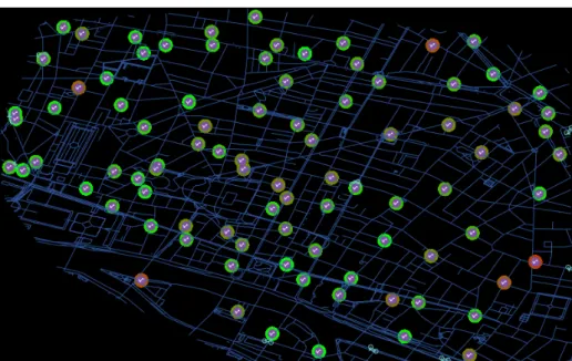
Concerning the choice of the level of representation in the graphical inter-face, we followed Banos in [25] when he argues that such exploratory models can really be exploited only if a feedback through the interface is possible. It is necessary to find a good compromise for the quantity of information displayed in
Fig. 2:Example of the graphical output of the model for a particular district (Chatelet). The map shows docking stations, for each the color gradient from green to red gives the current loading factor (green : empty, red : full).
the graphical interface. In our case, we represent a map of the district, on which link width is proportional to current flows, stations display their load-factor by a color code (color gradient from green, lf (s) = 0, to red, lf (s) = 1). Bikes are also represented in real time, what is interesting thanks to an option that allow to follow some individuals and visualize their decision process through arrows representing original destination, provenance and new destination (should be im-plemented in further work). This feature could be seen as superficial at this state of the work but it appears as essential regarding possible further developments of the project (see discussion section). Fig. 2 shows an example of the graphical interface of the implementation of the model of simulation.
Data collection All used data are open data, in order to have good reproducibility of the work. Road network vector layer was extracted from OpenStreetMap ([26]). Time-series of real stations statuts for Paris were collected automatically1
all 5 minutes during 6 month and were imported into R for treatment with [27] and the point dataset of stations was created from the geographical coordinates with [28].
Parametrization The model was designed in order to have real proxies for most of parameters. Mean travel speed is taken as ¯v =14km.h−1from [29], where data of trips where studied for the bike system of the city of Lyon, France. To simplify, we
1
take same speed for all bikers : v(b) = ¯v. A possible extension with tiny gaussian distribution around mean speed showed in experiments to bring nothing more. It has been shown in [3] that profiles of use of bike systems stays approximatively the same for european cities (but can be significantly different for cities as Rio or Taipei), what justify the use of these inferred data in our case. We also use the determined mean length of travel from [16] (here that parameter should be more sensible to the topology so we prefer extract it from this second paper although it seems to have subsequent methodological bias compared to the first rigorous work on the system of Lyon), which is 2.3km, in order to determine the diameter of the area on which our approach stays consistent. Indeed the model is built in order to have emphasis on travels coming from the outside and on travels going out, internal travels have to stay a small proportion of all travels. In our case, a district of diameter 2km gives a proportion of internal travels pit≈ 20%. We
will take districts of this size with this fixed proportion in the following.
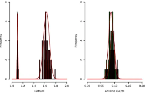
Detours Frequency 1.0 1.2 1.4 1.6 1.8 2.0 0 2 4 6 8 Adverse events Frequency 0.00 0.05 0.10 0.15 0.20 0 2 4 6 8
Fig. 3:Statistical analysis of outputs. For some aggregated outputs (here the overall quantity of detours and the pro-portion of adverse events), we plotted his-tograms of the statistical distribution of the functions on many realizations of the model for a point in the parameter space. Two points of the parameter space,
corre-sponding to (r = 300, pinf o = 50, σ = 80)
(green histogram) and (r = 700, pinf o =
50, σ = 80) (red) are plotted here as exam-ples. Gaussian fits are also drawn. The rela-tive good fit shows the internal consistence of the model and we are able to quantify the typical number of repetitions needed when applying the model : supposing normal dis-tributions for the indicator and its mean, a 95% confidence interval of size σ/2 is
ob-tained with n = (2 · 2σ ·1.96/σ)2≈ 60
The crucial part of the parametriza-tion is the construcparametriza-tion of O, D fields and random variables NI, ND from
real data. Daily data were reduced through sampling of time-series of load-factors of all stations and dimen-sion of the representation of a day was significantly reduced through a k-means clustering procedures (classi-cally used in time-series clustering as it is described in [30]). These reduced points were then clustered again in or-der to isolate typical weekdays from week-ends, where the use profiles are typically different and from special days such as ones with very bad cli-mate or public transportation strikes. That allowed to create the profile of a “standard day” that was used to infer O, D fields through a spatial Gaussian multi-kernel estimation (see [31]). The characteristic size of kernels 1/σ is an essential parameter for which we have no direct proxy, and that will have to be fixed through a calibration proce-dure. The laws for NI, NDwere taken
as binomial: for an actual arrival, we consider each possible travel and
in-crease the number of drawing of each binomial law of entries by 1 at the time corresponding to mean travel time (depending on the travel distance) before arrival time. Probabilities of binomial laws are 1/Card(I) since we assume
in-dependence of travels. For departure, we just increase by one drawings of the binomial law at current time for an actual departure.
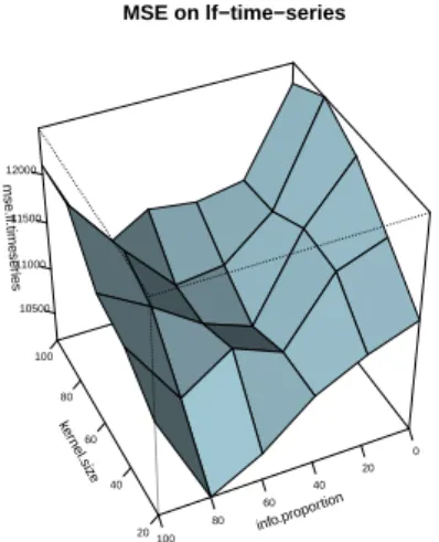
ker nel.siz e 20 40 60 80 100 info.propor tion 0 20 40 60 80 100 mse .lf .timeser ies 10500 11000 11500 12000 MSE on lf−time−series
Fig. 4:Simplified calibration procedure. We plot the surface of the mean-square er-ror on time-series of load-factors as a func-tion of the two parameters on which we want to calibrate. For visibility purpose, only one surface was represented out of the different obtained for different values of walking radius. The absolute minimum obtained for very large kernel has no sense since such value give quasi-uniform proba-bilities because of total recovering of Gaus-sian kernels. We take as best realization the second minimum, which is located around a kernel size of 50 and a quantity of informa-tion of 30%, which seem to be reasonable values afterwards.
What we call parameter space in the following consists in the 3 dimen-sional space of parameters that have not been fixed by this parametriza-tion, i. e. the walking radius r (taken as constant on all bikers, as for the speed), the information proportion pinf o what is the probability for a
new biker to have information and the ”size” of the Gaussian kernels σ (note that the spread of distributions is de-creasing with σ).
3.2 Robustness assessment, exploration and calibration Internal consistence of the model Be-fore using simulations of the model to explore possible strategies, it is nec-essary to assess that the results pro-duced are internally consistent, i. e. that the randomness introduced in the parametrization and in the internal rules do not lead to divergences in re-sults. Simulations were launched on a large number of repetitions for differ-ent points in the parameter space and statistical distribution of aggregated outputs were plotted. Fig. 3 shows ex-ample of these results. The relative good gaussian fits and the small devi-ation of distributions confirm the in-ternal consistence of the model. We obtain the typical number of repetitions needed to have a 95% confidence interval of length half of the standard devia-tion, what is around 60, and we take that number in all following experiments and applications. These experiments allowed a grid exploration of the parame-ter space, confirming expected behavior of indicators. In particular, the shape of M SE suggested to use the simplified calibration procedure presented in the following.
Robustness regarding the study area The sensitivity of the model regarding ge-ometry of the area was also tested. Experiments described afterwards were run on comparable districts (Chˆatelet, Saint-Lazare and Montparnasse), leading to the same conclusions, what confirms the external robustness of the model.
Reduced calibration procedure Using experiments launched during the grid ex-ploration of the parameter space, we are able to assess or the regularity of some aggregated criteria, especially of the mean-square error on loads factors of sta-tions. We calibrate on kernel size and quantity of information. For different values of the walking radius, the obtained area for the location of the minimum of the mean-square error stays quite the same for reasonable values of the ra-dius (300-600m). Fig. 4 shows an example of the surface used for the simplified calibration. We extract from that the values of around 50 for kernel size and 30 for information proportion. The most important is kernel size since we cannot have real proxy for that parameter. We use these values for the explorations of strategies in the following.
3.3 Investigation of user-based strategies
Influence of walking radius Taking for kernel-size and quantity of information the values given by the calibration, we can test the influence of walking radius on the performance of the system. Note that we make a strong assumption, that is that the calibration stay valid for different values of the radius. As we stand previously, this stays true as soon as we stay in a reasonable range of values (we obtained 300m to 600m) for the radius. The influence of variations of walking radius on indicators were tested. Most interesting results are shown in figure 5. Concerning the indicators evaluated on time-series (h and ¯l(t)), it is hard to have a significant conclusion since the small difference that one can observe between curves lies inside errors bars of all curves. For A, we see a decreasing of the indicator after a certain value (300m), what is significant if we consider that radius under that value are not realistic, since a random place in the city should be at least in mean over 300m from a bike station. However, the results concerning the radius are not so concluding, what could be due to the presence of periodic negative feedbacks: when the mean distance between two stations is reached, repartitions concerns neighbor stations as expected, but the relation is not necessarily positive, depending on the current status of the other station. A deeper understanding and exploration of the behavior of the model regarding radius should be the object of further work.
Influence of information For the quantity of information, we are on the contrary able to draw significant conclusions. Again, behavior of indicators were studied according to variations of pinf o. Most significant are shown on figure 6. Results
from time-series are also not concluding, but concerning aggregated indicators, we have a constant and regular decrease for each and for different values of the radius. We are able to quantify a critical value of the information for which most of the progress concerning indicator A (adverse events) is done, that is around 35%. We observe for this value an amelioration of 4% in the quantity of adverse events, that is interesting when compared to the total number of bikers. Regarding the management strategy for an increase in the level of service, that implies an increase of the penetration rate of online information tools (mobile
0.3 0.4 0.5 0.6 0.7 0 100 200 time heterogeneity 300 400 500 600 700 800 900 radius
(a) Time series of heterogeneity indica-tor h(t) for different values of walking radius. Small differences between means could mislead to a positive effect of radius on heterogeneity, but the error bars of all curves recover themselves, what makes any conclusion non-significant. 100 200 300 400 500 600 700 800 0.080 0.090 radius adv erse
(b) Influence of walking radius on the quantity of adverse events A. After 400m, we observe a relative decrease of the pro-portion. However, values under 300-400m should be ignored since these are smaller than the mean distance of a random point to a station.
Fig. 5: Results on the influence of walking radius.
application e. g.) if that rate is below 50%. If it is over that value, we have shown that efforts for an increase of penetration rate would be pointless.
4
Discussion
4.1 Applicability of the results
We have shown that increases of both walking radius and information quantity could have positive consequences on the level of service of the system, by reducing the overall number of adverse events and the quantity of detours especially in the case of the information. However, we can question the possible applicability of the results. Concerning walking radius, first a deeper investigation would be needed for confirmation of the weak tendency we observed, and secondly it appears that in reality, it should be infeasible to play on that parameter. The only way to approach that would be to inform users of the potential increase in the level of service if they are ready to make a little effort, but that is quite optimistic to think that they will apply systematically the changes, either because they are egoistic, because they won’t think about it, or because they will have no time.
Concerning the information proportion, we cannot also force users to have information device (although a majority of population owns such a device, they won’t necessarily install the needed software, especially if that one is not user-friendly). We should proceed indirectly, for example by increasing the ergonomics of the application. An other possibility would to improve information displayed at docking stations that is currently difficult to use.
0.06 0.08 0.10 0.12 0 25 50 75 100 info adv erse 300 400 500 600 700 radius
(a) Influence of proportion of information on adverse events A for two different val-ues of walking radius. We can conclude sig-nificantly that the information has a pos-itive influence. Quantitatively, we extract the threshold of 35% that corresponds to the majority of decrease, that means that more is not necessarily needed.
1.2 1.5 1.8 2.1 0 25 50 75 100 info detours 300 400 500 600 700 radius
(b) Influence of information on quantity of
detours Dtot. Curves for r = 300m and
r = 700m are shown (scale color). Here also, the influence is positive. The effect is more significant for high values of walk-ing radius. The inflection is around 50% of users informed, what is more than for adverse events.
Fig. 6: Results on the influence of proportion of information.
4.2 Possible developments
Other possible management strategies Concerning user parameters, other choices could have been made, as including waiting time at a fixed place, either for a parking or a bike. The parameters chosen are both possible to influence and quite adapted to the behavioral heuristic used in the model, and therefore were consid-ered. Including other parameters, or changing the behavioral model such as using discrete choice models may be possible developments of our work. Furthermore, only the role of user was so far explored. The object of further investigation could be the role of the “behavior” of docking stations. For example, one could fix rules to them, as close all parkings over a certain threshold of load-factor, or allow only departures or parkings in given configurations, etc. Such intelligent agents would surely bring new ways to influence the overall system, but will also increase the level of complexity (in the sense of model complexity, see [32]), and therefore that extension should be considered very carefully (that is the reason why we did not integrate it in this first work).
Towards an online bottom-up pilotage of the bike-sharing system Making the stations intelligent can imply making them communicate and behave as a self-adapting system. If they give information to the user, the heterogeneity of the nature and quantity of information provided could have strong impact on the overall system. That raises of course ethical issues since we are lead to ask if it is fair to give different quantities of information to different users. However, the perspective of a bottom-up piloted system could be of great interest from a theoretical and practical point of view. One could think of online adaptive algorithms for ruling the local behavior of the self-adapting system, such as ant
algorithms ([33]), in which bikers would depose virtual pheromones when they visit a docking station (corresponding to their information on travel that is easy to obtain), that would allow the system to take some local decisions of redirecting bikers or closing stations for a short time in order to obtain an overall better level of service. Such methods have already been studied to improve level of service in other public transportation systems like buses [34].
Conclusion
This work is a first step of a new bottom-up approach of bike-sharing systems. We have implemented, parametrized and calibrated a basic behavioral model and obtained interesting results for user-based strategies for an increase of the level of service. Further work will consist in a deeper validation of the model, its application on other data. We suggest also to explore developments such as extension to other types of agents (docking stations), or the study of possible bottom-up online algorithm for an optimal pilotage of the system.
References
1. Peter Midgley. The role of smart bike-sharing systems in urban mobility. JOUR-NEYS, 2:23–31, 2009.
2. Paul DeMaio. Bike-sharing: History, impacts, models of provision, and future. Journal of Public Transportation, 12(4):41–56, 2009.
3. Oliver O’Brien, James Cheshire, and Michael Batty. Mining bicycle sharing data for generating insights into sustainable transport systems. Journal of Transport Geography, 2013.
4. Zhili Liu, Xudong Jia, and Wen Cheng. Solving the last mile problem: Ensure the success of public bicycle system in beijing. Procedia-Social and Behavioral Sciences, 43:73–78, 2012.
5. Xue Geng, Kai TIAN, Yu ZHANG, and Qing LI. Bike rental station planning and design in paris [j]. Urban Transport of China, 4:008, 2009.
6. Jonathan Gifford and Arlington Campus. Will smart bikes succeed as public trans-portation in the united states? Center for Urban Transtrans-portation Research, 7(2):1, 2004.
7. Pierre Borgnat, Patrice Abry, and Patrick Flandrin. Mod´elisation statistique
cy-clique des locations de v´elo’v `a lyon. In XXIIe colloque GRETSI (traitement du
sig-nal et des images), Dijon (FRA), 8-11 septembre 2009. GRETSI, Groupe d’Etudes du Traitement du Signal et des Images, 2009.
8. Pierre Borgnat, Eric Fleury, C´eline Robardet, Antoine Scherrer, et al. Spatial
anal-ysis of dynamic movements of v´elo’v, lyon’s shared bicycle program. In European
Conference on Complex Systems 2009, 2009.
9. Pierre Borgnat, Patrice Abry, Patrick Flandrin, Jean-Baptiste Rouquier, et al.
Studying lyon’s v´elo’v: a statistical cyclic model. In European Conference on
Com-plex Systems 2009, 2009.
10. Pierre Borgnat, Patrice Abry, Patrick Flandrin, C´eline Robardet, Jean-Baptiste
Rouquier, and Eric Fleury. Shared bicycles in a city: A signal processing and data analysis perspective. Advances in Complex Systems, 14(03):415–438, 2011.
11. Andreas Kaltenbrunner, Rodrigo Meza, Jens Grivolla, Joan Codina, and Rafael Banchs. Urban cycles and mobility patterns: Exploring and predicting trends in a bicycle-based public transport system. Pervasive and Mobile Computing, 6(4):455– 466, 2010.
12. Jenn-Rong Lin, Ta-Hui Yang, and Yu-Chung Chang. A hub location inventory model for bicycle sharing system design: Formulation and solution. Computers & Industrial Engineering, 2011.
13. Jenn-Rong Lin and Ta-Hui Yang. Strategic design of public bicycle sharing sys-tems with service level constraints. Transportation research part E: logistics and transportation review, 47(2):284–294, 2011.
14. Alvina GH Kek, Ruey Long Cheu, and Miaw Ling Chor. Relocation simulation model for multiple-station shared-use vehicle systems. Transportation Research Record: Journal of the Transportation Research Board, 1986(1):81–88, 2006. 15. Rahul Nair and Elise Miller-Hooks. Fleet management for vehicle sharing
opera-tions. Transportation Science, 45(4):524–540, 2011.
16. Rahul Nair, Elise Miller-Hooks, Robert C Hampshire, and Ana Buˇsi´c. Large-scale
vehicle sharing systems: Analysis of v´elib’. International Journal of Sustainable
Transportation, 7(1):85–106, 2013.
17. Matthew Barth and Michael Todd. Simulation model performance analysis of a multiple station shared vehicle system. Transportation Research Part C: Emerging Technologies, 7(4):237–259, 1999.
18. Matthew Barth, Michael Todd, and Lei Xue. User-based vehicle relocation tech-niques for multiple-station shared-use vehicle systems. TRB Paper No. 04-4161, 2004.
19. Arnaud Banos, Annabelle Boffet-Mas, Sonia Chardonnel, Christophe Lang, Nicolas
Marilleau, Thomas Th´evenin, et al. Simuler la mobilit´e urbaine quotidienne: le
projet miro. Mobilit´es urbaines et risques des transports, 2011.
20. Patrick Vogel, Torsten Greiser, and Dirk Christian Mattfeld. Understanding bike-sharing systems using data mining: Exploring activity patterns. Procedia-Social and Behavioral Sciences, 20:514–523, 2011.
21. U. Wilensky. Netlogo. Center for Connected Learning and Computer-Based Mod-eling, Northwestern University, Evanston, IL., 1999.
22. QGIS Development Team. QGIS Geographic Information System. Open Source Geospatial Foundation, 2009.
23. R Core Team. R: A Language and Environment for Statistical Computing. R Foundation for Statistical Computing, Vienna, Austria, 2013.
24. Jan C Thiele, Winfried Kurth, and Volker Grimm. Agent-based modelling: Tools for linking netlogo and r. Journal of Artificial Societies and Social Simulation, 15(3):8, 2012.
25. Arnaud Banos. Pour des pratiques de mod´elisation et de simulation lib´er´ees en
G´eographie et SHS. PhD thesis, UMR CNRS G´eographie-Cit´es, ISCPIF, D´ecembre
2013.
26. Jonathan Bennett. OpenStreetMap. Packt Publishing, 2010.
27. Alex Couture-Beil. rjson: Json for r. R package version 0.2, 13, 2013.
28. Timothy H Keitt, Roger Bivand, Edzer Pebesma, and Barry Rowlingson. rgdal: bindings for the geospatial data abstraction library. R package version 0.7-1, URL http://CRAN. R-project. org/package= rgdal, 2011.
29. Pablo Jensen, Jean-Baptiste Rouquier, Nicolas Ovtracht, and C´eline Robardet.
Characterizing the speed and paths of shared bicycle use in lyon. Transportation research part D: transport and environment, 15(8):522–524, 2010.
30. T Warren Liao. Clustering of time series data—a survey. Pattern Recognition, 38(11):1857–1874, 2005.
31. Alexandre B Tsybakov. Introduction to nonparametric estimation. (introduction `
a l’estimation non-param´etrique.). 2004.
32. Franck Varenne, Marc Silberstein, et al. Mod´eliser & simuler. Epist´emologies et
pratiques de la mod´elisation et de la simulation, tome 1. 2013.
33. Nicolas Monmarch´e. Algorithmes de fourmis artificielles: applicationsa la
classifi-cation eta l’optimisation. PhD thesis, ´Ecole Polytechnique, 2004.
34. Carlos Gershenson. Self-organization leads to supraoptimal performance in public transportation systems. PLoS ONE, 6(6):e21469, 06 2011.