HAL Id: hal-01298942
https://hal.archives-ouvertes.fr/hal-01298942
Preprint submitted on 6 Apr 2016HAL is a multi-disciplinary open access archive for the deposit and dissemination of sci-entific research documents, whether they are pub-lished or not. The documents may come from teaching and research institutions in France or abroad, or from public or private research centers.
L’archive ouverte pluridisciplinaire HAL, est destinée au dépôt et à la diffusion de documents scientifiques de niveau recherche, publiés ou non, émanant des établissements d’enseignement et de recherche français ou étrangers, des laboratoires publics ou privés.
Multiple imputation for demographic hazard models
with left-censored predictor variables
Angela Greulich, Michael Rendall
To cite this version:
Angela Greulich, Michael Rendall. Multiple imputation for demographic hazard models with left-censored predictor variables. 2014. �hal-01298942�
Maryland Population Research Center
WORKING PAPER
Multiple imputation for demographic hazard models
with left-censored predictor variables
PWP-MPRC-2014-011 December 2014 Authors: Michael S. Rendall University of Maryland Angela Greulich Université Paris 1 Panthéon Sorbonne www.popcenter.umd.edu
Multiple imputation for demographic hazard models with left-censored predictor variables
Michael S. Rendall* and Angela Greulich**
December 13, 2014
Abstract
A common problem when using panel data is that an individual’s history is incompletely known at the first wave. We show that multiple imputation, the method commonly used for data that are missing due to non-response, may also be used to impute these data that are “missing by design.” Our application is to a woman’s duration of fulltime employment as a predictor of her risk of first birth. We multiply-impute employment status two years earlier to “incomplete” cases for which employment status is observed only in the most recent year. We then pool these
“completed” cases with the “complete” cases to derive regression estimates for the full sample. Relative to not being fulltime employed, having been fulltime-employed for two or more years is a positive and statistically significant predictor of childbearing whereas having just entered fulltime employment is not. The fulltime-employment duration parameter variances are about one third lower in the multiply-imputed sample than in the complete-data sample, and only in the multiply-imputed sample does the employment-duration coefficient attain statistical significance.
* Department of Sociology and Maryland Population Research Center, University of Maryland, College Park, USA
Acknowledgements: The data used in this study are from the European Commission, Eurostat,
longitudinal EU SILC years 2005-2012 (latest release and revision of earlier waves: October 2014). Eurostat has no responsibility for the results and conclusions of the authors.
1 INTRODUCTION
A common problem when using panel data for demographic applications is that the individual’s history is unknown or incompletely known at the first wave. In demographic hazard modeling, the length of time an individual has spent in a particular status or activity while exposed to the event of interest is often modeled. State histories may be collected retrospectively at the initial waves of panels surveys to overcome the problem that this duration is otherwise unknown. For example, fertility, marriage, migration, and employment histories are collected at or near the beginning of panel observation in the U.S. Survey of Income and Program Participation (U.S. Census Bureau 2014). State or event histories, however, are not always collected. Even when collected, not all characteristics of the history will be covered. For example, marital and fertility histories alone are not sufficient to identify co-residence histories between two parents and between each parent and child. In a previous treatment of this problem in the U.S. Panel Study of Income Dynamics, Moffitt and Rendall (1995) used a maximum likelihood approach to combine left-censored and non-left-censored spells of single motherhood in separate components of the likelihood. The statistical equivalence of maximum likelihood and multiple-imputation
approaches to handling missing data has been noted for cases of data that are missing due to non-response (Schafer and Graham 2002). The ability to separate the imputation step from the analysis step, however, is a major reason to prefer the multiple-imputation approach over the maximum likelihood approach.
Applying further the principles of missing-data analysis, questions that are asked for some individuals and not others in a survey result in a “missing by design” data pattern (Raghunathan and Grizzle 1995). One type of missing-by-design circumstance occurs in combined-survey analysis where the reason that data are missing for some individuals and not
2
others is because some individuals have been randomly sampled into one survey and whereas others have been randomly sampled into the other survey, and only one of the surveys includes a particular question from which a predictor variable is derived. Multiple imputation has been applied successfully to include such variables in pooled-sample analyses across a diverse set of substantive topics (Gelman, King, and Liu 1998; Rendall et al 2013; Van Hook et al
forthcoming).
When the reason that an observation is missing a particular variable is which survey the individual was sampled into, it will usually be clear that the missing at random (MAR)
assumption (Little and Rubin 2002), which is necessary for unbiased analysis with multiply-imputed data, will be satisfied. We argue that the MAR assumption will typically be satisfied also when a variable is missing due to left-censoring of a state history when a panel begins. For example, if age 16 is designated as the youngest possible age of employment, we may know for an individual who was age 16 at wave 1 how many years at age 20 he or she has been employed by wave 5 of an annual survey, whereas for an individual who was age 20 at wave 1, this
duration is unknown unless an employment history is collected. Whether a particular individual is 16 or 20 at the beginning of the survey may reasonably be treated as random for most
analytical purposes, and therefore the unknown employment duration of a 20 year old at wave 1 satisfies the MAR assumption. Despite the analytical attractiveness of their MAR pattern, we are unaware of any previous study that has applied the multiple-imputation approach to left-censored histories in the analysis of panel data.
We use a simple, but nevertheless realistic and widely-applicable example, in which individuals in a panel survey contribute either one or two waves of employment history with which to predict a partnered first birth. Our data source is the Poland country survey of the
3
European Union Survey on Income and Living Conditions (EU-SILC, Eurostat 2011a). Poland follows the standard format of including rotating panels, each including four annual waves. Using all four waves, we can use employment status in the first and second waves to predict births reported between the third and fourth waves. Using multiple imputation, however, we are additionally able to include birth-exposure intervals between the second and third wave in a model that uses employment status from two previous years. Compared with a model estimated with only birth-exposure intervals between the third and fourth waves, our parameter estimates are then derived from a sample whose number of person-year observations is twice as large. We discuss conditions under which the standard errors around the coefficients for duration employed (1 year only versus 2 or more years) may be accordingly reduced and find empirically that they are indeed substantially lower. Substantive implications from the multiply-imputed model results include that, whereas a woman’s having been employed fulltime for at least the last two years is statistically associated with a higher propensity to give birth, her having just entered a spell of fulltime employment is not. This result holds, moreover, when controlling for her partner’s employment status, a variable that is available in our panel data but that is typically not available in retrospective data.
DATA AND METHOD
The European Union Survey on Income and Living Conditions (EU-SILC) is a set of more than 30 country surveys conforming to a common format and content specified by Eurostat (Eurostat 2011a). The EU-SILC was created in 2003 as a replacement for the European Community
Household Panel (ECHP). It gathers harmonized and comparable data at the individual and at the household level on income and living conditions as well as on many individuals’ demographic
4
and socio-economic characteristics (sex, age, education, labor market position, etc.). The EU-SILC is composed of two datasets – one cross-sectional and one longitudinal (Eurostat 2011b). Subgroups of individuals observed in the cross-sectional dataset are followed up over several years to form the longitudinal dataset. The longitudinal design consists of a rotational panel in which individuals are observed annually for a standard maximum period of four years. The EU-SILC covers the majority of European countries for the years 2003 to 2012, although some began later than 2003, notably in 2005 when 10 new countries joined the European Union. For the present study, we use the longitudinal EU-SILC data for one country only, Poland, whose survey began in 2005. We choose Poland due to its relatively large number of observations (the number of observations available for each country reflects its population size, which was 38.5 million in 2011, Central Statistical Office of Poland 2012), and because the quality of the data has been assessed favorably (Iacovou, Kaminska, and Levy 2012). In particular, its wave-to-wave retention rate of approximately 90% is among the highest among EU-SILC countries. This retention rate exceeds that of all other larger countries in the EU-SILC. Selection into the Polish sample occurs annually, with each new sample followed for a further three waves. A stratified random sampling design ensures that sufficient sample sizes are attained for EU-designated “NUTS2” regions that are classified by degree of urbanization (Eurostat 2011a, p.33). We use sample weights that adjust for this design in the univariate descriptive statistics of our study.
We limit our analyses to partnered Polish women aged 18 to 39 who are observed for three or four consecutive waves between the years 2005 and 2012 and who are childless when entering the survey. The upper age restriction is needed so that we may reasonably approximate a woman’s being of parity 0 by her having no co-resident children. The restriction to individuals observed for a minimum of three waves is necessary since interviews usually take place during
5
the first half of each year children born in the third and the fourth quarters of each year are generally reported at the interview of the year after the birth. Two consecutive years of
interviews are then needed to identify all births that occur in one calendar year, and at least one more preceding wave is needed to observe the mother’s (and her partner’s) labor market status before exposure to conception and fertility. For those individuals who are observed for three waves, the latter two waves are designated 𝑡 and 𝑡 + 1 and serve to detect a first child arrival in the calendar year of wave 𝑡. Wave 𝑡 − 1 is used to observe the woman’s employment status and that of her partner. For those individuals who are observed for four waves and for whom no birth occurs in any of the calendar of the years of the first two waves, the woman’s employment status before birth exposure is observed in both waves 𝑡 − 2 and 𝑡 − 1.
An alternative data source for analyzing fertility by employment status in Poland, not used in the present study, is the retrospective 2006 Employment, Family, and Education Survey (EFES). The EFES was used by Matysiak (2009), who noted a disadvantage of that survey is its high rate of non-response among women’s partners (more than 50%), leading the author to analyze only women’s characteristics as predictors of their fertility. Contemporaneously-collected information on partners is a major advantage of panel data for the analysis of fertility by employment status and earnings (e.g., Adsera 2011).
Multiple Imputation (MI) for observations that are incomplete “by design”
We first describe the general “missing by design” setup and results already known with respect to efficiency gains from multiple imputation of missing data, and then proceed to the special case of incomplete information on employment-spell durations as predictor variables. We first specify a model with outcome variable 𝑌𝑡 for a birth in calendar year 𝑡 as a function of predictor
6
variables 𝑋𝑡−2 and 𝑋𝑡−1 observed respectively at times 𝑡 − 2 and 𝑡 − 1. The birth event is the result of a conception that will in most cases have occurred between 𝑡 − 1 and 𝑡. Our model therefore avoids predictor variables observed at time 𝑡, since it may not be clear what was the causal ordering between a conception carried to term, 𝑌𝑡, and a woman’s characteristics at time 𝑡, 𝑋𝑡. We use the binary logit model, LOGIT p[ ]=ln[ / (1p − p)], for the regression:
𝐿𝐿𝐿𝐿𝐿[Pr{𝑌𝑡|𝑋𝑡−2, 𝑋𝑡−1}] = 𝛽0+ 𝛽1𝑋𝑡−2+𝛽2𝑋𝑡−1 (1)
The data available to us to estimate this model are “complete” observations
{𝑌𝑡, 𝑋𝑡−2, 𝑋𝑡−1}𝑖=1𝑁1 and “incomplete” observations {𝑌𝑡, 𝑋𝑡−1}𝑗=1𝑁2 . We assume that the substantive
model represented by equation (1) applies equally to the complete and incomplete observations. This allows us to apply standard multiple imputation procedures to combine them in the analysis. Our specific application is as follows. We allow woman’s employment status 𝐸 to have an effect on 𝑌𝑡 based on its values at both times 𝑡 − 2 and 𝑡 − 1, 𝐸𝑡−2 and 𝐸𝑡−1. The other predictor variables in vector 𝑋, which we will henceforth denote by 𝑍, all have effects on 𝑌𝑡 only from their values at time 𝑡 − 1. Our variant of equation (1) is therefore:
𝐿𝐿𝐿𝐿𝐿[Pr {𝑌𝑡|𝐸𝑡−2, 𝐸𝑡−1, 𝑍𝑡−1} = 𝛽0+ 𝛽1𝐸𝑡−2+𝛽2𝐸𝑡−1+𝛽3𝑍𝑡−1 (1a)
We ignore item non-response, which is anyway very low for our variables of interest in the Poland EU-SILC, and assume that we have only “complete” observations
{𝑌𝑡, 𝐸𝑡−2, 𝐸𝑡−1, 𝑍𝑡−1}𝑖=1𝑁1 and “incomplete” observations {𝑌𝑡, 𝐸𝑡−1, 𝑍𝑡−1}𝑗=1𝑁2 . As a consequence,
the pattern of missingness is monotone (Little 1992) and we are able to apply a chained-equation multiple imputation approach (Raghunathan et al 2001) that allows for the imputation of binary, count, or continuous data. We use the set of complete observations to first estimate the
7
𝐿𝐿𝐿𝐿𝐿[Pr{𝐸𝑡−2|𝐸𝑡−1, 𝑍𝑡−1, 𝑌𝑡}] = 𝛾0+ 𝛾1𝐸𝑡−1+𝛾2𝑍𝑡−1+ 𝛾3𝑌𝑡 (2)
We then apply random draws from the posterior distribution of parameter estimates 𝛾�0, 𝛾�1, 𝛾�2, 𝛾�3 to the incomplete data {𝐸𝑡−1, 𝑍𝑡−1, 𝑌𝑡}𝑗=1𝑁2 to derive an arbitrarily large 𝑚 values of 𝐸𝑡−2 (we set 𝑚 = 20) to produce completed data {{𝑌𝑡(𝑘), 𝐸𝑡−2(𝑘), 𝐸𝑡−1(𝑘), 𝑍𝑡−1(𝑘)}𝑗=1𝑁2 }𝑘=1𝑚 . We then
concatenate the complete data {𝑌𝑡, 𝐸𝑡−2, 𝐸𝑡−1, 𝑍𝑡−1}𝑖=1𝑁1 to each instance of completed data and estimate the analysis equation (1a) 𝑚 times. These 𝑚 estimates of (1a) are combined using the standard multiple-imputation algorithms (Little and Rubin 2002) to produce a set of parameters with standard errors {𝛽̂0, 𝛽̂1, 𝛽̂2, 𝛽̂3; 𝑆𝐸(𝛽̂0), 𝑆𝐸(𝛽̂1), 𝑆𝐸(𝛽̂2), 𝑆𝐸(𝛽̂3)} that adjust for the
uncertainty introduced by imputation of 𝐸𝑡−2 to the incomplete person-year observations. This sequence of procedures may be performed with standard package software. We use SAS PROC MI and PROC MIANALYZE (SAS Institute 2008a, 2008b).
It is helpful to know generally what may be the efficiency gains from combining the complete and incomplete data. Equation (1) has been used in prior work to derive or estimate these expected efficiency gains. Little (1992) derived results in the linear regression case and White and Carlin (2010) did so additionally for the logistic regression case. A key parameter in evaluating efficiency gains obtained through multiply imputing is the “fraction missing.” In equation (1), there are only two predictors, one observed in both the complete and incomplete data, 𝑋𝑡−1, and another, 𝑋𝑡−2, observed only in the complete data. Following the terminology of White and Carlin, we define the fraction with missing values of 𝑋𝑡−2 by = 𝑁2/(𝑁1+ 𝑁2). The increase in sample size when both the complete and incomplete data are used in the estimation results in efficiency gains (reductions in standard errors or variances about the parameters) over an analysis that would estimate equation (1) from the complete data only. The larger the fraction
8
missing, the larger will be the efficiency gains. The largest variance reductions will be for 𝑉𝑉𝑉(𝛽̂2), the parameter for which the regressor variable (𝑋𝑡−1) is observed in both the complete
and incomplete data. Variance reduction about 𝑉𝑉𝑉(𝛽̂2) depends not only on the fraction missing π, however, but also on the correlation 𝜌122 between 𝑋𝑡−2 and 𝑋𝑡−1 and on the partial correlation
of 𝑌𝑡 and 𝑋𝑡−2 given 𝑋𝑡−1, 𝜌1𝑦.22 . Analytical expressions for the variance reductions about 𝑉𝑉𝑉(𝛽̂2) and 𝑉𝑉𝑉(𝛽̂1) are available in the linear case, originally from Little (1992). The
expression for the proportion by which 𝑉𝑉𝑉(𝛽̂2) is reduced by adding left-censored observations in the linear regression case is given by (White and Carlin 2010, p.2922):
𝜋(1 − 𝜌1𝑦.22 )[1 − 𝜌122 (1 − 2𝜌1𝑦.22 )] (3)
In the special case of no correlation between 𝑋𝑡−2 and 𝑋𝑡−1 and when 𝑋𝑡−2 has no association with 𝑌𝑡 independent of variation in 𝑋𝑡−2, then 𝑉𝑉𝑉(𝛽̂2) reduces by the maximum amount, equal to the fraction of left-censored observations, π. In this case, however, we could estimate β2 without the need for MI. Instead we would simply pool the complete and
incomplete data and estimate 𝐿𝐿𝐿𝐿𝐿[Pr {𝑌𝑡|𝑋𝑡−1} = 𝛽0+𝛽2𝑋𝑡−1. In the more general case of
2 1 .2
0<ρ y < and 1 2 12
0<ρ <1, the theoretical result is that MI will always result in a reduction in 𝑉𝑉𝑉(𝛽̂2) in the linear regression case because both (1 − 𝜌1𝑦.22 ) and [1 − 𝜌122 (1 − 2𝜌1𝑦.22 )] will
always be less than 1. Because they are greater than zero, the theoretical reduction in variance will be smaller than the fraction of left-censored observations, π. White and Carlin conduct simulations and real-data analyses and find that the variance reductions are typically close to (i.e., not much less than, and in some cases greater than) the fraction of missing values in both linear and logistic regression cases.
9
Reductions in 𝑉𝑉𝑉(𝛽̂1) are of particular interest because the coefficient 𝛽̂1 is associated with the variable 𝑋𝑡−2 for which data are partly missing. The reductions in variance about 𝛽̂1 are not generated directly, because only in the complete data is there any information about the relationship between 𝑌𝑡 and 𝑋𝑡−2. Instead, the only reduction in the variance of 𝑉𝑉𝑉(𝛽̂1) arises from the partial correlation of 𝑌𝑡 and 𝑋𝑡−2 given 𝑋𝑡−1, 𝜌1𝑦.22 . That is, efficiency may be gained by adding observations from the incomplete data (in our case, the left-censored observations) due to their indirectly providing information about the relationship between 𝑌𝑡 and 𝑋𝑡−2. This is
because 𝑋𝑡−2 and 𝑋𝑡−1 are correlated and this correlation carries with it information about variation in 𝑌𝑡 through providing information about the relationship between 𝑌𝑡 and 𝑋𝑡−1. The analytic expression for the variance reduction in 𝑉𝑉𝑉(𝛽̂1) in the linear regression case is, again originally from Little (1992):
2𝜋𝜌1𝑦.22 (1 − 𝜌1𝑦.22 ) (4)
In most cases, the value of this partial correlation will be low, and therefore negligible reduction in of 𝑉𝑉𝑉(𝛽̂1) is expected (e.g., White and Carlin 2010). In our case, however, the correlations between 𝑋𝑡−2 and 𝑋𝑡−1 and the partial correlation of 𝑌𝑡 and 𝑋𝑡−2 given 𝑋𝑡−1 are expected to be high, and therefore the reduction in 𝑉𝑉𝑉(𝛽̂1) potentially substantial. This is because our 𝑋𝑡−2 and 𝑋𝑡−1 are composites of employment status in times 𝑡 − 2 and 𝑡 − 1.
In particular, we consider three durations of fulltime-employment spells in progress at the time of birth exposure 𝐷𝑙: 0, 1, and 2 or more years. The reference category is 𝐷0 ≡ {1 𝑖𝑖 𝐸𝑡−1= 0 𝑉𝑎𝑎 0 𝑖𝑖 𝐸𝑡−1 = 1} and therefore requires only information from 𝑡 − 1. To code the alternate
categories, of duration exactly 1 year, 𝐷1, and duration of two or more years, 𝐷2, information at both times 𝑡 − 2 and 𝑡 − 1 is required, since 𝐷1 ≡ {1 𝑖𝑖 𝐸𝑡−1= 1 𝑉𝑎𝑎 𝐸𝑡−2 = 0} and 𝐷2 ≡ {1 𝑖𝑖 𝐸𝑡−1 = 1 𝑉𝑎𝑎 𝐸𝑡−2 = 1}. The analysis model we estimate is:
10
𝐿𝐿𝐿𝐿𝐿[Pr{𝑌𝑡|𝐷2, 𝐷1, 𝑍𝑡−1}] = 𝛽0+ 𝛽1𝐷2+𝛽2𝐷1+ 𝛽3𝑍𝑡−1 (1b)
Since reference duration category 𝐷0 and alternate duration categories 𝐷1 and 𝐷2 use both complete and multiply-imputed (“completed”) data for their coding, the expected efficiency gains in the estimation of 𝛽1 and 𝛽2 are a priori unknown. They are expected to be less,
however, than the efficiency gains in the estimation of 𝛽3. This is because 𝑍𝑡−1 is assumed to be non-missing for all observations, whereas both 𝐷1 and 𝐷2 are constructed partially from
observed data and partially from multiply-imputed data.
RESULTS
The sample consists of person-years exposed to a first birth among partnered, parity-0 women (see Table 1). Women’s mean age of exposure to first birth was 28.4 (from an observed age range of 20 to 39). We code employment status as either fulltime-employed or not for both the woman and her partner: 74.5% of women were fulltime-employed the year immediately
preceding a person-year of exposure to first birth, and 70.8% were fulltime-employed two years before the person-year of exposure to first birth; 85.9% of their partners were fulltime-employed the year immediately preceding their calendar year of exposure to first birth. Note that for only 200 person-years do we observe the woman’s employment status two years before their calendar year of exposure to first birth. Of a total of 671 person-year observations (maximum of two per woman), 323 were full-time employed in the year before birth exposure (𝑡 − 1) and did not have employment status observed in the year before that (𝑡 − 2) because they had not yet entered the panel. These are the left-censored spells. The “complete” data consist of 348 person-years, and thus the fraction with left-censored spells, referred to more generally as the fraction missing, is 0.481.
11
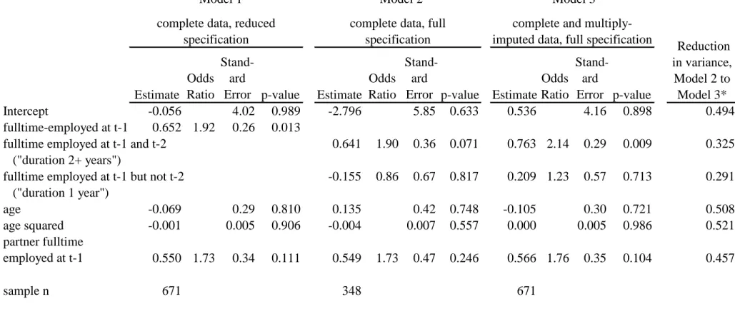
Regression results are presented in Table 2. We first use conventional methods to estimate models predicting a birth. These either simplify the specification of the employment-status predictor to use employment-status only at 𝑡 − 1 (Model 1) or use the fuller specification of
employment status at both 𝑡 − 1 and 𝑡 − 2, but necessarily for a person-year sample only half as large (Model 2). In the Model 1 estimation, in which all 671 person-years are used, but for which the specification of employment status is reduced to one prior year, being fulltime-employed at 𝑡 − 1 is a statistically-significant predictor of giving birth, associated with a 1.92 greater odds of giving birth compared to having not been fulltime-employed in the prior year. This result is consistent with Matysiak’s (2009) finding using retrospective data in the 2006 EFES survey, in which she also used employment status only in the year immediately before exposure.
When in Model 2 we distinguish between 1 year only of fulltime employment and 2 or more years of fulltime employment, we find that having been fulltime-employed 2 or more years (“duration 2+”) is associated with a 1.90 greater odds of giving birth compared to not having been fulltime-employed in the prior year (“duration 0”). This is statistically significant, however, only at the 0.10 level (p = 0.07). Women who entered fulltime employment in the most recent year (“duration 1”) did not have a statistically-significantly different likelihood of giving birth compared to women who were not fulltime-employed in the most recent year. These results are suggestive of duration of fulltime employment being a critical factor for predicting a partnered woman’s first birth. Using these conventional estimation methods, however, we are only able to include employment duration in the model at the cost of eliminating almost half of an already relatively small sample size, thereby rendering both employment-duration coefficients non-significant at conventional thresholds.
12
Our preferred model is Model 3, in which all 671 person-year observations are used, and with a specification of fulltime employment that distinguishes 0, 1, and 2+ years’ duration. This is the model made possible by multiply-imputing values of the fulltime-employed variable for the 323 person-years in which the woman was observed to be fulltime-employed at time 𝑡 − 1 and was not observed at time 𝑡 − 2. Our coefficient values are reassuring similar to those of Model 2, which used only complete data, indicating unbiased estimation with the multiply-imputed data. Model 3, however, has substantially lower standard errors than Model 2. This includes the standard error for the coefficient of greatest substantive interest to us, fulltime-employed for 2 or more years. Its standard error reduces from 0.36 in Model 2 to 0.29 in Model 3. Being fulltime-employed for 2 or more years is associated with a 2.14 greater odds of giving birth compared to not having been fulltime-employed in the prior year (“duration 0”), and the coefficient is now significant at the 0.01 level (p = 0.009). Entering fulltime employment in the most recent year (“duration 1”) was again not statistically-significant. In none of the three models is the coefficient for partner’s fulltime employment statistically significant, although it is in each case positive and with estimated magnitudes similar to those for the woman’s fulltime employment.
From prior theoretical and simulation studies cited above, the standard errors for the variables for which there are no missing values were expected to be much lower in the Model 3 than in the Model 2 estimates. In the linear regression case, the maximum theoretical reduction in variances (that is, the square of the standard error) is the proportion of cases that are missing, which in our case is 0.481 (being the fraction of person-years for which we cannot define the fulltime-employed duration as 0, 1, or 2+ years, see again Table 1). Although there is no such simple analytical expression in the logistic regression case, we see that the reduction in variances
13
for the age and age squared coefficients are 0.508 and 0.521, and so quite close to the fraction missing. The proportionate reduction in variance about the partner’s employment status is 0.457, again close to the fraction missing. Of greatest interest is the reduction in variances about the two employment spell duration coefficients. We expected that the reduction would be less than for those coefficients for variables that are constructed only from information at time 𝑡 − 1, and therefore non-missing, but we did not know by how much, nor even if there would be any substantial reduction in variances over the complete-data estimation. The proportionate reductions in variances are respectively 0.325 and 0.291 for the coefficients for fulltime employed two or more years and for fulltime employed only one year. These reductions are substantially less than the fraction missing, as expected, but are nevertheless surprisingly large magnitudes.
CONCLUSION
The use of multiple imputation in demographic research now spans at least 20 years (for early uses, see Freedman and Wolf 1995; Goldscheider et al 1999; and Sassler and McNally 2003). The standard use that is made of multiple imputation is to correct for various forms of non-response (see also Johnson and Young 2011). In the present study, we have argued that a promising additional use for multiple imputation is for data that are instead “missing by design” (Raghunathan and Grizzle 1995), in which the survey’s design means that only a fraction of the sample is asked a particular question. A major advantage of using MI for data that are missing by design is the expected validity of the assumption that data are missing at random (MAR). This assumption is both a requirement of, and is the biggest challenge for, the successful (unbiased) implementation of the method of multiple imputation (Schafer and Graham 2002). MI for
14
missing-by-design data patterns has previously been successfully implemented in combined-survey analysis (Gelman, King, and Liu 1998; Rendall et al 2013; Van Hook et al forthcoming), where the reason that data are missing for some individuals and not others is because some individuals have been randomly sampled into one survey and others have been randomly sampled into the other survey. We argue that left-censored spells beginning in the first wave of panel data are similarly likely to meet this MAR requirement because missingness again results from the random sampling process. The value of the MI method as applied in the present study is further enhanced by the ubiquity of left-censored spells beginning in the first wave of panel data. In short panels and in panels that sample from populations rather than from cohorts,
left-censored spells of employment and family status, for example, occur for almost every adult observed in the panel.
In the present study’s application of the MI method, we examined the gains that may be realized by multiply imputing a single additional year of employment status before the first wave of the panel. This amount of imputation was the maximum possible given the very short panel of our example data, the four-wave EU-SILC. Nevertheless, doing so allowed us to conduct a simple test of the hypothesis that women are more likely to begin childbearing after first
obtaining stable employment. Using conventional methods to conduct this test would have meant using only half the number of person-year observations that we were able to use in our multiply-imputed data analysis. Alternative data or analytical methods that could instead have been used all have limitations. To proxy for stability of employment as a predictor of fertility when no employment history was collected in the European Community Household Panel (ECHP), Santarelli (2011, p.322) used a variable for type of employment contract (permanent or
15
for it is not consistently available across countries. Özcan, Mayer, and Luedicke (2010) criticized studies that ignore problems of left-censoring and instead used a cross-sectional survey, the German Life History Survey, with employment and demographic histories. The life histories collected in cross-sectional surveys, however, have major limitations, notably that they often include little or no recording of the employment statuses of current and former partners.
In the empirical part of our study, we found that a woman’s being newly fulltime-employed was not predictive of a first birth whereas being fulltime-fulltime-employed for two or more years was strongly predictive of a first birth. In terms of the estimated coefficient sign and magnitude, we found this result to be consistent between estimation using the larger set of person-years that we “completed” by multiple imputation and estimation using the smaller set of “complete” person-years in which the employment spell of up to two years was observed. This concordance in estimates between the complete-data and multiply-imputed data analyses is reassuring from the perspective of protecting against any bias that might be induced by the multiple imputation of data from the complete observations to the incomplete observations. Only in the analysis with the multiply-imputed data, however, was this key substantive coefficient statistically significant at conventional levels (p < .05). The magnitude of variance reduction about the parameter was around one third. To have obtained a variance reduction of this size represents a substantial payoff to having multiply-imputed a variable for employment status two years before the birth exposure for such a large fraction of our person-year sample. This large amount of variance reduction, moreover, was not easily knowable in advance of our conducting the study, since the left-censored spell case of the present study is qualitatively different from those for which previous work has derived expected variance reductions (e.g., White and Carlin 2010). We attribute the large variance reduction to the fact that for every observation at least
16
some information was available on the length of the spell. Future work, however, might profitably investigate the different amounts of variance reduction that may be realized under different types and magnitudes of missing versus non-missing information in left-censored histories.
REFERENCES
Adsera, A. (2011) The interplay of employment uncertainty and education in explaining second births in Europe Demographic Research 25(16):513-544.
Central Statistical Office of Poland (2012) Demographic Yearbook of Poland 2012 http://stat.gov.pl/en/topics/population/population/ Accessed 12/12/2014. Eurostat (2011a) “2008 Comparative EU Final Quality Report,” Version 3, July 2011. Eurostat (2011b) “Description of target variables: Cross-sectional and Longitudinal”, 2011
operation (Version May 2011).
Freedman, V.A., and D.A. Wolf (1995) A case study on the use of multiple imputation
Demography 32:459-470.
Gelman, A., G. King, and C. Liu (1998a) Not asked and not answered: Multiple imputation for multiple surveys Journal of the American Statistical Association 94(443):846-857. Goldscheider, F., C. Goldscheider, P. St. Clair, and J. Hodges (1999) Changes in returning home
in the United States, 1925-1985 Social Forces 78(2):695-720.
Gonzalez, M.-J. and Jurado-Guerrero, T. (2006) Remaining childless in affluent economies: A comparison of France, West Germany, Italy and Spain, 1994-2001 European Journal of
17
Iacovou, M. O. Kaminska, and H. Levy (2012) “Using EU-SILC data for cross-national analysis: strengths, problems and recommendations” Institute for Social and Economic Research Working Paper Series No. 2012-03, Essex University.
Johnson, D.R., and R. Young (2011) Toward best practices in analyzing datasets with missing data: Comparisons and recommendations Journal of Marriage and Family 73: 926-945. Little, R.J.A. (1992) Regression with missing X’s: A review Journal of the American Statistical
Association 87(420):1227-1237.
Little, R.J.A., and D.B. Rubin (2002) Statistical Analysis with Missing Data (2nd Edition)
Hoboken, NJ: Wiley.
Matysiak, A. (2009) Employment first, then childbearing: Women’s strategy in post-socialist Poland Population Studies 63(3):253-276.
Moffitt, R.A., and M.S. Rendall (1995) Cohort trends in the lifetime distribution of female family headship in the U.S., 1968-85 Demography 32(3):407-424.
Özcan, B., K. Ulrich Mayer, and J. Luedicke (2010) The impact of unemployment on the transition to parenthood Demographic Research 23:807-846.
Raghunathan, T.E., and J.E. Grizzle (1995) A split questionnaire survey design Journal of the
American Statistical Association 94(447):896-908.
Raghunathan, T.E., J.M. Lepkowski, J. van Hoewyk, and P. Solenberger (2001) A multivariate technique for multiply imputing missing values using a sequence of regression models
Survey Methodology 27(1):85-95.
Rendall, M.S., B. Ghosh-Dastidar, M.M. Weden,E.H. Baker, and Z. Nazarov (2013)Multiple imputation for combined-survey estimation with incomplete regressors in one but not both surveys Sociological Methods and Research 42(4):483-530.
18
Santarelli, E. (2011) Economic resources and the first child in Italy: A focus on income and job stability Demographic Research 25:311-336.
SAS Institute (2008a) “The MI Procedure” Ch.54 SAS/STAT 9.2 User Guide, 2nd Ed.
SAS Institute (2008b) “The MIANALYZE Procedure” Ch.55 SAS/STAT 9.2 User Guide, 2nd Ed.
Sassler S., and J. McNally (2003) Cohabiting couples’ economic circumstances and union transitions: a re-examination using multiple imputation techniques Social Science
Research 32(4):553-578.
Schafer, J.L., and J.W. Graham (2002) Missing data: Our view of the state of the art
Psychological Methods 7(2):147-177.
U.S. Census Bureau (2014) “SIPP Introduction and History” http://www.census.gov/programs-surveys/sipp/about/sipp-introduction-history.html# Accessed 10/13/2014.
Van Hook, J., J.D. Bachmeier, D. Coffman, and O. Harrel (forthcoming) Can We Spin Straw Into Gold? An Evaluation of Legal Status Imputation Approaches Demography. White, I.R., and J.B. Carlin (2010) Bias and efficiency of multiple imputation compared with
Mean Standard deviation Sample size 28.7 4.4 671 0.745 0.436 671 0.708 0.456 200 0.859 0.349 671
Left censored observations: fulltime employed at t-1, not observed at t-2 323
Non-left-censored observations 348
All observations 671
Fraction missing full-time employment duration (left-censored) 0.481
Source: European Union Survey of Income and Living Conditions, Poland 2005-2012
Note: all observations have valid values of age and partner's employment status at t-1 and of birth
between t and t+1
Numbers of observations (unweighted person-years)
Table 1 Descriptive statistics and numbers of observations, partnered parity-0 Polish women, 2005-2012
Descriptive statistics (person-years, weighted)
woman's age
woman's fulltime employment in t-1 (proportion) woman's fulltime employment in t-2 (proportion) partner's fulltime employment in t-1 (proportion)
Estimate
Odds Ratio
Stand-ard
Error p-value Estimate
Odds Ratio
Stand-ard
Error p-value Estimate Odds Ratio Stand-ard Error p-value Intercept -0.056 4.02 0.989 -2.796 5.85 0.633 0.536 4.16 0.898 0.494 fulltime-employed at t-1 0.652 1.92 0.26 0.013
fulltime employed at t-1 and t-2 0.641 1.90 0.36 0.071 0.763 2.14 0.29 0.009 0.325
("duration 2+ years")
fulltime employed at t-1 but not t-2 -0.155 0.86 0.67 0.817 0.209 1.23 0.57 0.713 0.291 ("duration 1 year") age -0.069 0.29 0.810 0.135 0.42 0.748 -0.105 0.30 0.721 0.508 age squared -0.001 0.005 0.906 -0.004 0.007 0.557 0.000 0.005 0.986 0.521 partner fulltime employed at t-1 0.550 1.73 0.34 0.111 0.549 1.73 0.47 0.246 0.566 1.76 0.35 0.104 0.457 sample n 671 348 671 Notes:
Source: European Union Survey of Income and Living Conditions, Poland 2005-2012
* calculated by squaring the Standard Errors and taking the proportionate reduction in these variances about the parameter estimate from Model 2 to Model 3
Model 1 Model 2 Model 3
Table 2 Logistic regressions of birth in year t, before and after imputing fulltime employment status in t-2, partnered parity-0 Polish women, 2005-2012
Reduction in variance, Model 2 to Model 3* complete data, reduced
specification
complete data, full specification
complete and multiply-imputed data, full specification